Macroscopic reduction for stochastic reaction-diffusion equations

Abstract

The macroscopic behavior of dissipative stochastic partial differential equations usually can be described by a finite dimensional system. This article proves that a macroscopic reduced model may be constructed for stochastic reaction-diffusion equations with cubic nonlinearity by artificial separating the system into two distinct slow-fast time parts. An averaging method and a deviation estimate show that the macroscopic reduced model should be a stochastic ordinary equation which includes the random effect transmitted from the microscopic timescale due to the nonlinear interaction. Numerical simulations of an example stochastic heat equation confirms the predictions of this stochastic modelling theory. This theory empowers us to better model the long time dynamics of complex stochastic systems.

Key Words: Stochastic reaction-diffusion equations averaging, tightness, martingale.

AMS Subject Classifications: 60H15, 35K57, 92E20.

1 Introduction

Stochastic partial differential equations (spdes) are widely studied in modeling, analyzing, simulating and predicting complex phenomena in many fields of nonlinear science [8, 9, 19, e.g.].

Reaction-diffusion equations (rdes) are important mathematic models naturally applied in chemistry, biology, geology, physics and ecology etc. Such equations can be obtained from microscopic particle systems under the so called hydrodynamic space-time scaling limit [5] . When taking fluctuations under the hydrodynamic limit into account, an additive noise appears as correction term to the reaction-diffusion equation [1]. This reaction-diffusion equation with noise is viewed as an equation describing intermediate level between the macroscopic and microscopic ones. A deterministic equation appears in the macroscale only if the randomness averages out.

However, for nonlinear complex systems, random effects may survive averaging and thus be fed into the macroscopic system [17]. Especially when we consider the macroscopic behavior of solution on a long time scale, such random effects should not be neglected [12, 15, 17, e.g.]. Furthermore, macroscopic turbulence may need to be modeled as noise in, for example, geophysical fluid dynamics.

Blömker et al. [2, 4, e.g.] recently studied amplitude equations for spdes with cubic nonlinearity, which is proved to be a stochastic Landau equation. But in the amplitude equation the fluctuation from the fast modes disappears when the noise just acts on fast modes. For spdes with quadratic nonlinearity, Roberts [13] derived the amplitude equation for one dimensional stochastic Burgers equations by calculating a stochastic normal form model. Blömker et al. [3] also gave a rigorous proof for a general spdes with quadratic nonlinearity by a multiscale analysis; they showed that the amplitude equations include the fluctuation from the fast mode due to the nonlinearity interaction.

This paper considers reaction-diffusion systems driven by a noise which is homogeneous in space and white in time. Here we are concerned with the dynamics of the system on a long time scale. For this, a scale transformation separates the system into slow and fast modes. Then we derive a low dimension macroscopic system which provides the long term dynamics. And the low dimensional macroscopic system includes a noise term which is transmitted from the fast modes due to nonlinear interaction.

For definiteness, let the non-dimensional $I=(0,\pi)$ and $L^{2}(I)$ be the Lebesgue space of square integrable real valued functions on $I$ . Consider the following non-dimensional reaction-diffusion equation

$$\partial_{t}w = \partial_{xx}w+f(w)+\sigma\partial_{t}W\quad\text{on}\;\;0<x<\pi\,,$$ (1)

$$w = 0\quad\text{on}\;\;x=0\,,\;\pi\,,$$ (2)

where $f(w)$ represents a nonlinear reaction and $W$ is an $L^{2}(I)$ valued $Q$-Wiener process defined on complete probability space $(\Omega,\mathcal{F},\mathbb{P})$ which is detailed in the next section. Our aim is to study the behavior of solutions to (1)–(2) over a large timescale, say $\epsilon^{-1}$ for small $\epsilon>0$ . For some fixed integer $N>0$ , we split the field $w$ into $N$ low wavenumber modes and the remaining high wavenumber modes. For this non-dinesional problem, denote by $\{e_{k}(x)\}_{k}=\{\sin(kx)\}_{k}$ the orthonormal eigenvectors of $\partial_{xx}$. Define the projection operators onto ‘slow’ and ‘fast’ modes respectively

$$\mathcal{P}_{N}\cdot=\sum_{k=1}^{N}e_{k}(x)\langle e_{k}(x)\,,\cdot\rangle\,,\quad\mathcal{Q}_{N}=\mathcal{I}-\mathcal{P}_{N}\,,$$ (3)

where $\mathcal{I}$ is the identity operator on $L^{2}(I)$ . Then defining $u=\mathcal{P}_{N}w$ and $v=\mathcal{Q}_{N}w$ , the rde (1) is identical to the following coupled equations

$$\partial_{t}u = \partial_{xx}u+\mathcal{P}_{N}f(u+v)+\sigma\mathcal{P}_{N}\partial_{t}W\,,$$ (4)

$$\partial_{t}v = \partial_{xx}v+\mathcal{Q}_{N}f(u+v)+\sigma\mathcal{Q}_{N}\partial_{t}W\,,$$ (5)

whence $w=u+v$ . In order to completely separate the time scales we modify the above system by introducing a ‘high-pass filter’ $A_{N}$ defined by

$$A_{N}=\partial_{xx}-(1-\epsilon)\mathcal{P}_{N}\partial_{xx}=(\mathcal{Q}_{N}+\epsilon\mathcal{P}_{N})\partial_{xx}\,.$$

Observed that when $\epsilon=1$ , the physical case, the operator $A_{N}=\partial_{xx}$ as appears in (1) and (4)–(5); but when $\epsilon=0$ , the operator $A_{N}$ is a pure high-pass filter with null space spanned of the ‘slow’ modes.

For the moment also assume the noise acts only on the high wavenumber modes, that is $\mathcal{P}_{N}W=0$ . And modify the system (4)–(5) to

$$\partial_{t}u^{\epsilon} = A_{N}u^{\epsilon}+\mathcal{P}_{N}f(u^{\epsilon}+v^{\epsilon})\,,$$ (6)

$$\partial_{t}v^{\epsilon} = A_{N}v^{\epsilon}+\mathcal{Q}_{N}f(u^{\epsilon}+v^{\epsilon})+\sigma\sqrt{\epsilon}\mathcal{Q}_{N}\partial_{t}W\,.$$ (7)

Here the choice of $\sqrt{\epsilon}$, the factor in front of noise term, ensures the fast modes, solutions of (7), remain of order $1$ as $t\rightarrow\infty$ and $\epsilon\rightarrow 0$ for any fixed $u^{\epsilon}$ . Note that when $\epsilon=1$ , (6)–(7) is identical to (4)–(5) and (1). We aim to use analysis based upon small $\epsilon$ to access a useful approximation at $\epsilon=1$ .

Section 5.1 proves that, for small enough $\epsilon>0$ , high modes $v^{\epsilon}(t)$ is approximated by $\sqrt{\epsilon}\eta_{*}(t)$ over long timescales ($1/\epsilon$) where $\eta_{*}$ is the stationary solution solving the linear stochastic partial differential equation

$$\partial_{t}\eta=A_{N}\eta+\sigma\mathcal{Q}_{N}\partial_{t}W\,.$$ (8)

Consequently our careful averaging proves that the macroscopic behavior of $u^{\epsilon}(t)$ is described to a first approximation by $\sqrt{\epsilon}u_{N}(\epsilon t)$ which solves the following finite dimensional, deterministic system

$$\partial_{t}u_{N}=\partial_{xx}u_{N}+\mathcal{P}_{N}\overline{f_{0}}(u_{N})\,.$$ (9)

Here, the average

$$\overline{f_{0}}(u_{N})=\lim_{t\rightarrow\infty}\frac{1}{t}\int_{0}^{t}f_{0}(u_{N}+\eta_{*}(s))ds\,,$$ (10)

and $f_{0}$ is the cubic component in $f$, see detail in next section. Usually (9) is called the averaged equation and in probability the following convergence holds (Section 5.2): for any $T>0$ there is positive constant $C$

$$\sup_{0<t<\epsilon^{-1}T}|u^{\epsilon}(t)-\sqrt{\epsilon}u_{N}(\epsilon t)|_{L^{2}(D)}\leq C\epsilon$$ (11)

for small $\epsilon$ under some proper conditions on the initial value. Further, the martingale approach of Section 5.3 shows that small Gaussian fluctuations generally appear in these slow modes on the timescale $\epsilon^{-1}$. The approach shows that fluctuations are transmitted from the fast modes by nonlinear interactions. The last Section 6 confirms these theoretical predictions by comparing them to numerical simulations of a specific stochastic reaction diffusion equation.

2 Preliminaries and main results

This section gives some preliminaries and states the main result. First we give some functional background and some assumptions.

Let $H=L^{2}(I)$. Denote by $A$ the second order operator $\partial_{xx}$ with Dirichlet boundary on $I$ and let $\{e_{i}\}_{i=1}^{\infty}$ be a eigen-basis of $H$ such that

$$Ae_{i}=-\alpha_{i}e_{i}\,,\quad i=1,2,\ldots\,,$$

with $0<\alpha_{1}<\alpha_{2}<\alpha_{3}<\cdots$. For any $\delta>0$ , introduce the space $H^{\delta}_{0}=D(A^{\delta/2})$, which is compactly embedding into $H$. And let $H^{-\delta}$ denote the dual space of $H_{0}^{\delta}$. The usual norm defined on $H^{\delta}$ is written as $\|\cdot\|_{\delta}$. And for $\delta=0$ and $1$, the corresponding norms are written as $|\cdot|$ and $\|\cdot\|$ respectively. Denote by $\langle\cdot,\cdot\rangle$ an inner product in $H$ such as the inner product $\left<u,v\right>=(2/\pi)\int_{0}^{\pi}uv\,dx$ . And for positive integer $N$, denote by $H_{N}$ the space spanned by $\{e_{1},\ldots,e_{N}\}$ and by $H_{N}^{\perp}$ the space spanned by $\{e_{N+1},\ldots\}$ .

We are given a complete probability space $(\Omega,\mathcal{F},\{\mathcal{F}_{t}\}_{t\geq 0},\mathbb{P})$. Assume $W$ is an $H$-valued $Q$-Wiener process with operator $Q$ that commutes with $\mathcal{P}_{N}$ and satisfies

$$Qe_{i}=\lambda_{i}e_{i}\,,\quad i=1,2,\ldots\,,$$

with $\lambda_{i}=0$ , $i=1,2,\ldots\,,N$ and $\lambda_{i}>0$ , $i=N+1,\ldots$ . Then

$$W(t)=\sum_{i=N+1}^{\infty}\sqrt{\lambda_{i}}\beta_{i}(t)e_{i}$$ (12)

where component noises

$$\beta_{i}(t)=\frac{1}{\sqrt{\lambda_{i}}}\langle W(t),e_{i}\rangle\,,\quad i=N+1,\ldots\,,$$

are real valued Brownian motions mutually independent on $(\Omega,\mathcal{F},\mathbb{P})$. Moreover we assume

$$\operatorname{tr}Q=\sum_{i=N+1}^{\infty}\lambda_{i}<\infty.$$ (13)

In the following we denote by $Q_{2}=(I-\mathcal{P}_{N})Q=Q$ . For the nonlinear term $f$ we assume the following hypotheses $(\textbf{H})$

1. $f:{\mathbb{R}}\rightarrow{\mathbb{R}}$ is smooth and has the following form

   $$f(\xi)=f_{0}(\xi)+f_{1}(\xi)\,,\quad\xi\in{\mathbb{R}}\,,$$

   where $f_{0}(\xi)=-c_{0}\xi^{3}$ , $c_{0}$ is some positive constant, $f^{\prime\prime\prime}_{1}(0)=0$ and $f_{1}(\xi)\xi\leq 0$ , $\xi\in{\mathbb{R}}$ .

2. $f^{\prime}(\xi)<c_{1}$ for some positive constant $c_{1}$ .

3. There are positive constants $c_{2}$ , $c_{3}$ and positive integer $p$ such that for $\xi\in{\mathbb{R}}$

   $$|f(\xi)|\leq c_{2}|\xi|^{2p-1}+c_{3}\,,\quad f(\xi)\xi\leq c_{2}\xi^{2p}+c_{3}\,.$$

4. $(f(\xi)-f(\delta))(\xi-\eta)\leq 0\,,\quad\xi,\eta\in{\mathbb{R}}\,.$

Then define

$$f^{\epsilon}(\xi)=\frac{1}{\epsilon\sqrt{\epsilon}}f(\sqrt{\epsilon}\xi)$$ (14)

which is well-defined as $\epsilon\rightarrow 0$ for any $\xi\in{\mathbb{R}}$ by the above assumptions. Then $f^{\epsilon}$ satisfies the hypotheses (H) with $f_{1}$ replaced by $f_{1}^{\epsilon}(\xi)=f_{1}(\sqrt{\epsilon}\xi)/\epsilon\sqrt{\epsilon}$ .

Remark 1.

One example for such $f$ is the following polynomial with only negative odd order terms

$$f(\xi)=-a_{1}\xi^{3}-\cdots-a_{p}\xi^{2p-1}$$

where $a_{i}>0$ , $i=1,\ldots,p$ .

Now we state the main result of this paper.

Theorem 2.

Assume the Wiener process $W$ satisfies assumption (13). Then for any time $T>0$ and constant $R>0$, there is positive constant $C>0$ , such that for any solution $(u^{\epsilon}(t),v^{\epsilon}(t))$ of (6)–(7) with initial value $|(u_{0},v_{0})|\leq\sqrt{\epsilon}R$ , there is a $N$-dimensional Wiener process $\bar{W}$ such that in distribution

$$\sup_{0\leq t\leq\epsilon^{-1}T}|u^{\epsilon}(t)-\sqrt{\epsilon}u_{N}(\epsilon t)-\epsilon\rho_{N}(\epsilon t)|\leq C\epsilon^{1+}\,.$$ (15)

Here $u_{N}$ solves (9) and $\rho_{N}$ solves the following stochastic differential equations

$$\partial_{t}\rho_{N}=A_{N}\rho_{N}+\mathcal{P}_{N}[\overline{f^{\prime}_{0}}(u_{N})\rho_{N}]+\sqrt{B(u_{N})}\,\partial_{t}\bar{W}\,,$$ (16)

with $\rho_{N}(0)=0$ and

$$\overline{f^{\prime}_{0}}(u_{N})=\lim_{t\rightarrow\infty}\frac{1}{t}\int_{0}^{t}f^{\prime}_{0}(u_{N}+\eta_{*}(s))ds$$

and

$$B(u_{N}) = 2\int_{0}^{\infty}\mathbb{E}\Big{[}\mathcal{P}_{N}f_{0}(u_{N}+\eta_{*}(t))-\mathcal{P}_{N}\overline{f_{0}}(u_{N})\Big{]}$$

$${}\otimes\Big{[}\mathcal{P}_{N}f_{0}(u_{N}+\eta_{*}(0))-\mathcal{P}_{N}\overline{f_{0}}(u_{N})\Big{]}dt\,,$$

where $\otimes$ is the tensor product. Furthermore

$$\mathbb{E}\sup_{0\leq t\leq\epsilon^{-1}T}|v^{\epsilon}(t)-\sqrt{\epsilon}\eta_{*}(t)|\leq C\epsilon\sqrt{\epsilon}\,.$$ (17)

Now we introduce some scale transformations such that system (6)–(7) is defined on time scale $\epsilon^{-1}$ under the transformations. Introduce slow time $t^{\prime}=\epsilon t$ and small fields $u^{\epsilon}=\sqrt{\epsilon}u^{\prime\epsilon}(x,t^{\prime})$ and $v^{\epsilon}=\sqrt{\epsilon}v^{\prime\epsilon}(x,t^{\prime})$ . Substituting and hereafter omitting primes, the coupled system (6)–(7) is transformed to the following stochastic reaction diffusion equation with clearly separated time scales:

$$\partial_{t}u^{\epsilon} = \partial_{xx}u^{\epsilon}+\mathcal{P}_{N}f^{\epsilon}(u^{\epsilon}+v^{\epsilon})\,,$$ (18)

$$\partial_{t}v^{\epsilon} = \frac{1}{\epsilon}\partial_{xx}v^{\epsilon}+\mathcal{Q}_{N}f^{\epsilon}(u^{\epsilon}+v^{\epsilon})+\frac{\sigma}{\sqrt{\epsilon}}\mathcal{Q}_{N}\partial_{t}W\,,$$ (19)

with $u^{\epsilon}(0,t)=u^{\epsilon}(\pi,t)=v^{\epsilon}(0,t)=v^{\epsilon}(\pi,t)=0$ for $t>0$ . The Wiener process $W$ is a rescaled version of (12) and with the same distribution.

For convenience in the following we rewrite (18)–(19) into the following form

$$\partial_{t}w^{\epsilon}=A_{\epsilon}w^{\epsilon}+f^{\epsilon}(w^{\epsilon})+\Sigma_{\epsilon}\partial_{t}{W}\,,\quad\text{on}\quad 0<x<\pi\,.$$ (20)

Here $A_{\epsilon}=(\partial_{xx}\,,\epsilon^{-1}\partial_{xx})$ with zero Dirichlet boundary condition.

In order to approximate solutions of (6)–(7), our basic idea is to pass limit $\epsilon\rightarrow 0$ in (18)–(19) to determine interesting structure in solutions, then study the deviation between the limit and solution. This first step is to give compact estimates, that is, tightness of solutions, as addressed in the following two sections.

3 Stochastic convolution

Start by considering the linear stochastic equation

$$\partial_{t}z^{\epsilon}=A_{\epsilon}z^{\epsilon}+\Sigma_{\epsilon}\partial_{t}{W},\quad z^{\epsilon}(0)=0\,.$$

Let $S_{\epsilon}(t)$ be the analytic semigroup generated by $A_{\epsilon}$, then in a mild sense

$$z^{\epsilon}(t)=\int_{0}^{t}S_{\epsilon}(t-s)\Sigma_{\epsilon}dW(s).$$ (21)

For any $T>0$ and $\delta>0$ , we give a uniform estimates for $z(t)$, $0<t<T$, in space $H^{\delta}_{0}$. We have

Theorem 3.

Assume (13). Then for any $T>0$ , $q>0$ , there is positive constant $C_{q}(T)$ such that

$$\mathbb{E}\sup_{0\leq t\leq T}\|z^{\epsilon}(t)\|^{q}\leq C_{q}(T).$$ (22)

Proof.

By using the stochastic factorization formula [7], for $\alpha\in(0,1/2)$ we have

$$z^{\epsilon}(t)=\frac{\sin\pi\alpha}{\pi}\int_{0}^{t}(t-s)^{\alpha-1}S_{\epsilon}(t-s)Y^{\epsilon}_{\alpha}(s)ds$$

where

$$Y_{\alpha}^{\epsilon}(s)=\int_{0}^{s}(s-r)^{-\alpha}S_{\epsilon}(s-r)\Sigma_{\epsilon}\,dW(r).$$ (23)

Now for $q>1/\alpha$ , we have by the definition of $A_{\epsilon}$

$$\|z^{\epsilon}(t)\|^{q}_{\delta} \leq c_{q}\Big{[}\int_{0}^{t}(t-s)^{\frac{(\alpha-1)q}{q-1}}ds\Big{]}^{q-1}\int_{0}^{t}\big{\|}S_{\epsilon}(t-s)Y_{\alpha}^{\epsilon}(s)\big{\|}^{q}_{\delta}\,ds$$

$$\leq c_{q}(T)\int_{0}^{t}\|Y_{\alpha}^{\epsilon}(s)\|^{q}_{\delta}\,ds$$

for some positive constant $c_{q}(T)$. Then we have

$$\mathbb{E}\sup_{0\leq t\leq T}\|z^{\epsilon}(t)\|^{q}_{\delta}\leq c_{q}(T)\mathbb{E}\int_{0}^{T}\|Y^{\epsilon}_{\alpha}(s)\|^{q}_{\delta}\,ds\,.$$

By the definition of $A_{\epsilon}$, rewrite (23) as

$$Y_{\alpha}^{\epsilon}(s)=\sum^{\infty}_{i=N+1}\sigma\sqrt{\lambda_{i}}e_{i}\int_{0}^{s}(s-r)^{-\alpha}e^{-\alpha_{i}(s-r)/\epsilon}\epsilon^{-1/2}d\beta_{i}(r).$$

Then if $q>4$, by the Bukholder–Davies–Gundy inequality we have

$$\mathbb{E}\|Y^{\epsilon}_{\alpha}(s)\|^{q}_{\delta} = \mathbb{E}\Big{\|}\int_{0}^{s}(s-r)^{-\alpha}S_{\epsilon}(s-r)\Sigma_{\epsilon}\,dW(r)\Big{\|}_{\delta}^{q}$$

$$\leq c_{q}\Big{[}\sum_{i=N+1}^{\infty}\sigma^{2}\lambda_{i}\alpha_{i}^{\delta}\int_{0}^{s}(s-r)^{-2\alpha}e^{-2\alpha_{i}(s-r)/\epsilon}\epsilon^{-1}\,dr\Big{]}^{q/2}$$

$$\leq c_{q}(s)\sigma^{q}\Big{[}\sum_{i=1}^{\infty}\lambda_{i}\alpha_{i}^{\delta-1}\Big{]}^{q/2}.$$

Therefore there is positive constant $C_{q}(T)$, independent of $\epsilon$, such that

$$\mathbb{E}\sup_{0\leq t\leq T}\|z^{\epsilon}(t)\|^{q}_{\delta}\leq c_{q}(T)\mathbb{E}\int_{0}^{T}\|Y^{\epsilon}_{\alpha}(s)\|^{q}_{\delta}\,ds\leq C_{q}(T).$$

By the assumption (13), taking $\delta\leq 1$ and the Young inequality yields the result (22) for all $q>0$ . ∎

4 Tightness of solutions

This section gives a tightness result by some a priori estimates for solutions to (18)–(19) and the estimate of Theorem 3.

Define $\tilde{w}^{\epsilon}=w^{\epsilon}-z^{\epsilon}$, then by (20)

$$\partial_{t}\tilde{w}^{\epsilon}=A_{\epsilon}\tilde{w}^{\epsilon}+f^{\epsilon}(w^{\epsilon})$$ (24)

which is equivalent to

$$\partial_{t}\tilde{u}^{\epsilon} = \partial_{xx}\tilde{u}^{\epsilon}+\mathcal{P}_{N}f^{\epsilon}(w^{\epsilon})\,,$$

$$\partial_{t}\tilde{v}^{\epsilon} = \epsilon^{-1}\partial_{xx}\tilde{v}^{\epsilon}+\mathcal{Q}_{N}f^{\epsilon}(w^{\epsilon})$$

with zero Dirichlet boundary condition on $(0,\pi)$ and $\tilde{w}^{\epsilon}=\tilde{u}^{\epsilon}+\tilde{v}^{\epsilon}$ .

Then we have for some positive constants $c_{4}$ and $c_{5}$

$$\frac{1}{2}\frac{d}{dt}|\tilde{w}^{\epsilon}|^{2} = -\|\tilde{u}^{\epsilon}\|^{2}-\epsilon^{-1}\|\tilde{v}^{\epsilon}\|^{2}+\langle f^{\epsilon}(w^{\epsilon}),\tilde{w}^{\epsilon}\rangle$$

$$= -\|\tilde{u}^{\epsilon}\|^{2}-\epsilon^{-1}\|\tilde{v}^{\epsilon}\|^{2}+\langle f^{\epsilon}(w^{\epsilon}),w^{\epsilon}\rangle-\langle f^{\epsilon}(w^{\epsilon}),z\rangle$$

$$\leq -\|\tilde{w}^{\epsilon}\|^{2}-c_{2}|w^{\epsilon}|^{2p}_{L^{2p}(I)}+c_{3}\pi+\left(c_{2}|w^{\epsilon}|^{2p-1}_{L^{2p}(I)}+c_{3}\pi^{1/(2p)^{\prime}}\right)|z|_{L^{(2p)^{\prime}}(I)}$$

$$\leq -\|\tilde{w}^{\epsilon}\|^{2}-c_{4}|w^{\epsilon}|^{2p}_{L^{2p}(I)}+c_{5}\left(|z|^{2p}_{L^{(2p)^{\prime}}(I)}+1\right).$$

Integrating with respect to time yields

$$\sup_{0\leq t\leq T}|\tilde{w}^{\epsilon}(t)|^{2}+2\int_{0}^{T}\|\tilde{w}^{\epsilon}(s)\|^{2}\,ds+2c_{4}\int_{0}^{T}|w^{\epsilon}(s)|^{2p}_{L^{2p}(I)}\,ds$$ (25)

$$\leq |w_{0}|^{2}+2c_{5}\int_{0}^{T}|z^{\epsilon}(s)|^{2p}_{L^{(2p)^{\prime}}(I)}ds+2c_{5}T$$

$$\leq |w_{0}|^{2}+2c_{5}\int_{0}^{T}\|z^{\epsilon}(s)\|^{2p}\,ds+2c_{5}T.$$

On the other hand we have a positive constant $c_{5}$ such that

$$\frac{1}{2}\frac{d}{dt}\|\tilde{w}^{\epsilon}\|^{2} = -\langle A_{\epsilon}\tilde{w}^{\epsilon},\Delta\tilde{w}^{\epsilon}\rangle-\langle f^{\epsilon}(w^{\epsilon}),\Delta w^{\epsilon}+\Delta z^{\epsilon}\rangle$$

$$\leq -|\Delta\tilde{w}^{\epsilon}|^{2}+c_{1}\|\tilde{w}^{\epsilon}\|^{2}+\left(c_{2}|w^{\epsilon}|^{2p-1}_{L^{2p}(I)}+c_{3}\pi^{1/(2p)^{\prime}}\right)\|z^{\epsilon}\|_{L^{(2p)^{\prime}}(I)}$$

$$\leq -|\Delta\tilde{w}^{\epsilon}|^{2}+c_{1}\|\tilde{w}^{\epsilon}\|^{2}+|w^{\epsilon}|^{2p}_{L^{2p}(I)}+c_{6}\left(\|z^{\epsilon}\|^{2p}_{L^{(2p)^{\prime}}(I)}+1\right)\,.$$

Integrating with respect to time yields

$$\sup_{0\leq s\leq t}\|\tilde{w}^{\epsilon}(s)\|^{2} \leq \|w_{0}\|^{2}+2c_{1}\int_{0}^{t}\sup_{0\leq\tau\leq s}\|\tilde{w}^{\epsilon}(\tau)\|^{2}\,ds+2\int_{0}^{T}|w^{\epsilon}(s)|^{2p}_{L^{2p}(I)}\,ds$$

$${}+2c_{6}\int_{0}^{T}\|z^{\epsilon}(s)\|^{2p}_{L^{(2p)^{\prime}}(I)}\,ds+2c_{6}T.$$

Then by the Gronwall lemma and (25),

$$\sup_{0\leq t\leq T}\|\tilde{w}^{\epsilon}(t)\|^{2}\leq c_{7}T\left(1+\|w_{0}\|^{2}+\int_{0}^{T}\|z^{\epsilon}(s)\|^{2p}\,ds\right)$$ (26)

for some positive constant $c_{7}$. Further for any integer $m\geq 1$ ,

$$\frac{d}{dt}[\|\tilde{w}^{\epsilon}\|^{2}]^{m}\leq C_{m}\big{[}\|\tilde{w}^{\epsilon}\|^{2m}+\|\tilde{w}^{\epsilon}\|^{2m-2}|w^{\epsilon}|^{2p}_{L^{2p}(I)}+\|z^{\epsilon}\|^{2mp}+1\big{]}.$$

Then

$$\sup_{0\leq s\leq t}\|\tilde{w}^{\epsilon}(s)\|^{2m}$$

$$\leq C_{m}\int_{0}^{t}\sup_{0\leq\tau\leq s}\|\tilde{w}^{\epsilon}(\tau)\|^{2m}\,ds+C_{m}\sup_{0\leq\tau\leq T}\|\tilde{w}^{\epsilon}(\tau)\|^{2m-2}\int_{0}^{T}|w^{\epsilon}(s)|^{2p}_{L^{2p}(I)}\,ds+$$

$$C_{m}\int_{0}^{T}\|z^{\epsilon}(s)\|^{2mp}\,ds+C_{m}T+\|w_{0}\|^{2m}.$$

By induction on $m$, we derive that

$$\sup_{0\leq t\leq T}\|\tilde{w}^{\epsilon}(t)\|^{2m}\leq C_{m}T\Big{(}1+\|w_{0}\|^{2m}+\int_{0}^{T}\|z^{\epsilon}(t)\|^{2mp}\,dt\Big{)}$$ (27)

for some positive constant $C_{m}$.

Now we show $\{\mathcal{L}(w^{\epsilon})\}_{\epsilon}$, the distribution of $w^{\epsilon}$, is tight in $C(0,T;H)$. For this we need the following lemma by Simon [16].

Lemma 4.

Assume $E$, $E_{0}$ and $E_{1}$ be Banach spaces such that $E_{1}\Subset E_{0}$, the interpolation space $(E_{0},E_{1})_{\theta,1}\subset E$ with $\theta\in(0,1)$ and $E\subset E_{0}$ with $\subset$ and $\Subset$ denoting continuous and compact embedding respectively. Suppose $p_{0}$, $p_{1}\in[1,\infty]$ and $T>0$, such that

$$\mathcal{V}\;{\textrm{i}s\;a\;bounded\;set\;in\;}L^{p_{1}}(0,T;E_{1})$$

and

$$\partial\mathcal{V}:=\{\partial v:v\in\mathcal{V}\}\;{\textrm{i}s\;a\;bounded\;set\;in\;}L^{p_{0}}(0,T;E_{0}).$$

Here $\partial$ denotes the distributional derivative. If $1-\theta>1/p_{\theta}$ with

$$\frac{1}{p_{\theta}}=\frac{1-\theta}{p_{0}}+\frac{\theta}{p_{1}}\,,$$

then $\mathcal{V}$ is relatively compact in $C(0,T;E)$.

Now by the above lemma, noticing the estimate (22) and $w^{\epsilon}=\tilde{w}^{\epsilon}-z^{\epsilon}$, we draw the following result

Theorem 5.

Assume (13). For any $T>0$ , $\{\mathcal{L}(w^{\epsilon})\}_{\epsilon}$ is tight in $C(0,T;H)$ .

5 Macroscopic reduction

In this section we prove the main result. First Section 5.1 approximates the high modes by the Gaussian process $\eta^{\epsilon}$. Then Section 5.2 derives an averaged approximation for the low modes, and the fluctuation is considered in Section 5.3.

5.1 Approximation for high modes

We consider the high frequency dynamics of (19). First for any fixed $u\in H_{N}$ , $v^{\epsilon}$ satisfies

$$\partial_{t}v^{\epsilon}=\frac{1}{\epsilon}\partial_{xx}v^{\epsilon}+\mathcal{Q}_{N}f^{\epsilon}(u+v^{\epsilon})+\frac{\sigma}{\sqrt{\epsilon}}\partial_{t}{W}.$$ (28)

For any $v_{0},v_{1}\in H_{N}^{\perp}$, we have

$$|v^{\epsilon}(t;v_{0})-v^{\epsilon}(t;v_{1})|^{2}\leq e^{-2\alpha_{N+1}t/\epsilon}|v_{0}-v_{1}|^{2}$$

which means a unique stationary solution $\tilde{v}^{\epsilon}_{u}$ exists for any fixed $u$. In the following we determine the limit of $\tilde{v}^{\epsilon}_{u}$ in $C(0,T;H_{N}^{\perp})$ as $\epsilon\rightarrow 0$ for any $u\in H_{N}$ .

For this we scale time for equation (8) by $t^{\prime}=\epsilon t$ which yields, upon omitting primes,

$$\partial_{t}\eta=\frac{1}{\epsilon}\partial_{xx}\eta+\frac{\sigma}{\sqrt{\epsilon}}\partial_{t}W.$$ (29)

Here $W$ is a rescaled version of the noise process in (8) and with the same distribution. Then $\eta^{\epsilon}_{*}(t)=\eta^{*}(t/\epsilon)$ is the unique stationary solution of (29). Moreover $\eta_{*}^{\epsilon}$ is an exponential mixing Gaussian process with distribution $\mu=\mathcal{N}\big{(}0,\sigma^{2}(-A)^{-1}Q_{2}/2\big{)}$.

Now we prove that for any $u\in H_{N}$ , $\tilde{v}_{u}^{\epsilon}$ could be approximated by $\eta^{\epsilon}$ as $\epsilon$ is small. Let $V^{\epsilon}=v^{\epsilon}-\eta^{\epsilon}$, then

$$\partial_{t}V^{\epsilon}=\frac{1}{\epsilon}\partial_{xx}V^{\epsilon}+\mathcal{Q}_{N}f^{\epsilon}(u+v^{\epsilon}),\quad V^{\epsilon}(0)=v(0)-\eta^{\epsilon}(0).$$

Multiplying $V^{\epsilon}$ on both sides of above equation in $H$ yields

$$\frac{d}{dt}|V^{\epsilon}|^{2}\leq-\frac{\alpha_{N+1}}{\epsilon}|V^{\epsilon}|^{2}+\frac{\epsilon}{2\alpha_{N+1}}|f^{\epsilon}(u+v^{\epsilon})|^{2}.$$ (30)

Then by the Gronwall lemma and (27), there is positive constant $C$ such that for any $t>0$

$$\mathbb{E}|V^{\epsilon}(t)|^{2} \leq e^{-\alpha_{N+1}t/\epsilon}\mathbb{E}|v(0)-\eta_{*}(0)|^{2}+$$

$$\quad\frac{\epsilon}{2\alpha_{N+1}}\int_{0}^{t}e^{-\alpha_{N+1}(t-s)/\epsilon}\mathbb{E}|f^{\epsilon}(u+v^{\epsilon}(s))|^{2}\,ds$$

$$\leq \epsilon^{2}C\big{(}\|w(0)\|^{2p}+\mathbb{E}|\eta_{*}(0)|^{2}\big{)}.$$

Furthermore by

$$V^{\epsilon}(t)=e^{At/\epsilon}V^{\epsilon}(0)+\int_{0}^{t}e^{A(t-s)/\epsilon}\mathcal{Q}_{N}f^{\epsilon}(u+v^{\epsilon}(s))ds$$

for any $T>0$ , there is positive constant $C_{T}$ such that

$$\mathbb{E}\sup_{0\leq t\leq T}|v^{\epsilon}(t)-\eta_{*}^{\epsilon}(t)|\leq\epsilon C_{T}\big{(}\|w_{0}\|^{2p}+\mathbb{E}|\eta_{*}(0)|\big{)}\,.$$

This proves (17).

We end this subsection by giving an estimate on $|V^{\epsilon}(t)|^{2m}$ , $m>0$ , which is used in the fluctuation estimate in Section 5.3. By (30) we have

$$\frac{d}{dt}|V^{\epsilon}|^{2m} \leq -\frac{m\alpha_{N+1}}{\epsilon}|V^{\epsilon}|^{2m}+\frac{\epsilon}{2\alpha_{N+1}}|V^{\epsilon}|^{2m-2}|f(u+v^{\epsilon})|^{2}$$

$$\leq -\frac{m\alpha_{N+1}}{2\epsilon}|V^{\epsilon}|^{2m}+\epsilon C_{m}|f(u+v^{\epsilon})|^{2m}$$

for some positive constant $C_{m}>0$ . Then by the Hölder inequality, Gronwall lemma and (27) we have

$$\mathbb{E}|V^{\epsilon}(t)|^{2m}\leq C_{m}\,,\quad t\geq 0\,.$$ (31)

5.2 Averaged equation

In order to pass limit $\epsilon\rightarrow 0$ , we restrict our system into a small probability space. By the estimates in Section 4, for any $\kappa>0$ there is a compact set $B_{\kappa}\subset C(0\,,T\,;H)$ such that

$$\mathbb{P}\{u^{\epsilon}\in B_{\kappa}\}>1-\kappa\,.$$

Furthermore there is positive constant $C_{T}^{\kappa}$, such that

$$\|u^{\epsilon}(t)\|^{2}\leq C_{T}^{\kappa}\,,\quad t\in[0,T],$$

for any $u^{\epsilon}\in B_{\kappa}$. Now we introduce the probability space ($\Omega_{\kappa}\,,\mathcal{F}_{\kappa}\,,\mathbb{P}_{\kappa}$) defined by

$$\Omega_{\kappa}=\{\omega\in\Omega:u^{\epsilon}\in B_{\kappa}\}\,,\quad\mathcal{F}_{\kappa}=\{S\cap\Omega_{\kappa}:S\in\mathcal{F}\}$$

and

$$\mathbb{P}_{\kappa}(S)=\frac{\mathbb{P}(S\cap\Omega_{\kappa})}{\mathbb{P}(\Omega_{\kappa})}\,,\text{ for }S\in\mathcal{F}_{\kappa}\,.$$

Then $\mathbb{P}(\Omega\setminus\Omega_{\kappa})\leq\kappa$ .

Now we restrict $\omega\in\Omega_{\kappa}$ and introduce an auxiliary process. For any $T>0$ , partition the interval $[0,T]$ into subintervals of length $\delta=\sqrt{\epsilon}$ . Then we construct processes $(\tilde{u}^{\epsilon},\tilde{v}^{\epsilon})$ such that for $t\in[k\delta,(k+1)\delta)$,

$$\tilde{u}^{\epsilon}(t) = e^{A(t-k\delta)}u^{\epsilon}(k\delta)+\int_{k\delta}^{t}e^{A(t-s)}\mathcal{P}_{N}f^{\epsilon}(u^{\epsilon}(k\delta),\tilde{v}^{\epsilon}(s))\,ds\,,$$ (32)

$$\tilde{u}^{\epsilon}(0)=u_{0}\,,$$

$$\partial_{t}\tilde{v}^{\epsilon}(t) = \frac{1}{\epsilon}\partial_{xx}\tilde{v}^{\epsilon}(t)+\mathcal{Q}_{N}f^{\epsilon}(u^{\epsilon}(k\delta),\tilde{v}^{\epsilon}(t))+\frac{\sigma}{\sqrt{\epsilon}}\mathcal{Q}_{N}\,\partial_{t}{W}(t)\,,$$ (33)

$$\tilde{v}^{\epsilon}(k\delta)=v^{\epsilon}(k\delta)\,.$$

Then by the Itô formula for $t\in[k\delta,(k+1)\delta)$,

$$\frac{1}{2}\frac{d}{dt}|v^{\epsilon}(t)-\tilde{v}^{\epsilon}(t)|^{2}$$

$$\leq -\frac{\lambda_{N+1}}{\epsilon}|v^{\epsilon}(t)-\tilde{v}^{\epsilon}(t)|^{2}+\big{\langle}f^{\epsilon}(u^{\epsilon}(t)\,,v^{\epsilon}(t))-f^{\epsilon}(u^{\epsilon}(t)\,,\tilde{v}^{\epsilon}(t)),v^{\epsilon}(t)-\tilde{v}^{\epsilon}(t)\big{\rangle}$$

$${}+\big{\langle}f^{\epsilon}(u^{\epsilon}(t)\,,\tilde{v}^{\epsilon}(t))-f^{\epsilon}(u^{\epsilon}(k\delta)\,,\tilde{v}^{\epsilon}(t))\,,v^{\epsilon}(t)-\tilde{v}^{\epsilon}(t)\big{\rangle}$$

$$\leq -\frac{\lambda_{N+1}}{2\epsilon}|v^{\epsilon}(t)-\tilde{v}^{\epsilon}(t)|^{2}+\epsilon\left(c_{2}\|w^{\epsilon}(t)\|^{2p}+c_{3}\right)|u^{\epsilon}(t)-\tilde{u}^{\epsilon}(k\delta)|^{2}\,.$$

By the choice of $\Omega_{\kappa}$, there is $C_{T}>0$ , such that

$$|u^{\epsilon}(t)-u^{\epsilon}(k\delta)|^{2}\leq C_{T}\delta^{2}\,,\quad\text{for}\;t\in[k\delta,(k+1)\delta)\,.$$ (34)

Then by the Gronwall lemma,

$$|v^{\epsilon}(t)-\tilde{v}^{\epsilon}(t)|^{2}\leq C_{T}\delta^{2}\,,\quad t\in[0,T]\,.$$ (35)

In a mild sense for $t\in[k\delta,(k+1)\delta)$

$$u^{\epsilon}(t)=e^{A(t-k\delta)}u^{\epsilon}(k\delta)+\int_{k\delta}^{t}e^{A(t-s)}\mathcal{P}_{N}f^{\epsilon}(u^{\epsilon}(s),v^{\epsilon}(s))\,ds\,.$$

Then by the cubic property of $f$ and smoothing property of $e^{At}$, noticing the choice of $\Omega_{\kappa}$, we have for $t\in[k\delta,(k+1)\delta)$

$$|u^{\epsilon}(t)-\tilde{u}^{\epsilon}(t)| \leq C^{\prime}\int_{k\delta}^{t}|v^{\epsilon}(s)-\tilde{v}^{\epsilon}(s)|\,ds+C^{\prime}\int_{k\delta}^{t}|u^{\epsilon}(k\delta)-u^{\epsilon}(s)|\,ds$$

for some positive constant $C^{\prime}$ . So by (35) we have

$$|u^{\epsilon}(t)-\tilde{u}^{\epsilon}(t)|\leq C_{T}\delta\,,\quad t\in[0\,,T]\,.$$ (36)

On the other hand, in a mild sense the solution of (9) is

$$u_{N}(t)=e^{At}u_{0}+\int_{0}^{t}e^{A(t-s)}\mathcal{P}_{N}\overline{f_{0}}(u_{N}(s))\,ds\,.$$

Then, using $\lfloor z\rfloor$ to denote the largest integer less than or equal to $z$,

$$|\tilde{u}^{\epsilon}(t)-u_{N}(t)| \leq \int_{0}^{t}e^{A(t-s)}\big{|}\mathcal{P}_{N}f^{\epsilon}(u^{\epsilon}(\lfloor s/\delta\rfloor\delta),\tilde{v}^{\epsilon}(s))-\mathcal{P}_{N}\overline{f^{\epsilon}}(u^{\epsilon}(\lfloor s/\delta\rfloor\delta))\big{|}ds$$

$${}+\int_{0}^{t}e^{A(t-s)}\big{|}\mathcal{P}_{N}\overline{f^{\epsilon}}(u^{\epsilon}(\lfloor s/\delta\rfloor\delta))-\mathcal{P}_{N}\overline{f_{0}}(u^{\epsilon}(s))\big{|}ds$$

$${}+\int_{0}^{t}e^{A(t-s)}\big{|}\mathcal{P}_{N}\overline{f_{0}}(u^{\epsilon}(s))-\mathcal{P}_{N}\overline{f_{0}}(u_{N}(s))\big{|}ds\,.$$

Notice $\eta$ is independent of $\epsilon$, by the assumption H, and $\mathcal{P}_{N}\overline{f^{\epsilon}}$ is continuous in $\epsilon$. Moreover the exponential mixing stationary measure $\mu$ is independent of $u$, by the ergodic theorem

$$\overline{f_{0}}(u_{N})=\lim_{t\rightarrow\infty}\frac{1}{t}\int_{0}^{t}f_{0}(u_{N}+\eta_{*}(s))ds=\int_{H_{N}^{\perp}}f_{0}(u_{N}+v)\mu(dv)\,.$$

Then for any $u_{1}$ , $u_{2}\in H_{N}$

$$\Big{|}\int_{H_{N}^{\bot}}[f_{0}(u_{1},v)-f_{0}(u_{2},v)\big{]}\mu(dv)\Big{|}$$ (37)

$$\leq 2c_{0}\Big{|}\int_{H_{N}^{\bot}}(u_{1}-u_{2})(u^{2}_{1}+u_{2}^{2}+v^{2})\mu(dv)\Big{|}$$

$$\leq 2c_{0}\Big{[}\|u_{1}\|^{2}+\|u_{2}\|^{2}+\mathbb{E}\|\eta^{*}\|^{2}\Big{]}|u_{1}-u_{2}|\,$$

which yields the continuity of $\mathcal{P}_{N}\overline{f}_{0}\,:H_{N}\rightarrow H_{N}$ . Then we have for $t\in[0,T]$

$$|\tilde{u}^{\epsilon}(t)-u_{N}(t)|\leq C_{T}\left[\delta+\int_{0}^{T}|u^{\epsilon}(s)-u_{N}(s)|\,ds\right]\,.$$ (38)

As

$$|u^{\epsilon}(t)-u_{N}(t)|\leq|u^{\epsilon}(t)-\tilde{u}(t)|+|\tilde{u}(t)-u_{N}(t)|\,,$$

by the Gronwall lemma and (34), (36) and (38) we have for $t\in[0,T]$,

$$|u^{\epsilon}(t)-u_{N}(t)|\leq C_{T}\sqrt{\epsilon}\,.$$ (39)

Now by the arbitrariness of $\kappa$, we complete the proof of the averaging approximation. And since $\eta_{*}$ is Gaussian with zero mean, we give

$$\mathcal{P}_{N}\overline{f_{0}}(u_{N})=-c_{0}\mathcal{P}_{N}(u_{N}^{3}+3u_{N}\mathbb{E}\bar{\eta}^{2})\,.$$ (40)

5.3 Fluctuation

This subsection details the approximation of $u^{\epsilon}$ for small $\epsilon$. We study the deviation between $u^{\epsilon}$ and $u$, which proves to be a Gaussian process. This shows that there are fluctuations in the slow modes. We follow an approach used previously [17, 10, 18]. For this define the scaled difference

$$\bar{\rho}^{\epsilon}=\frac{1}{\sqrt{\epsilon}}(u^{\epsilon}-u_{N})\,.$$

Then $\bar{\rho}^{\epsilon}$ solves

$$\partial_{t}\bar{\rho}^{\epsilon}=\partial_{xx}\bar{\rho}^{\epsilon}+\frac{1}{\sqrt{\epsilon}}\big{[}\mathcal{P}_{N}f^{\epsilon}(u^{\epsilon},v^{\epsilon})-\mathcal{P}_{N}\overline{f^{\epsilon}}(u_{N})\big{]}\,,\quad\bar{\rho}^{\epsilon}(0)=0\,.$$

However, here we just consider $\rho^{\epsilon}$, the solution of

$$\partial_{t}\rho^{\epsilon}=\partial_{xx}\rho^{\epsilon}+\frac{1}{\sqrt{\epsilon}}\big{[}\mathcal{P}_{N}f_{0}(u^{\epsilon},v^{\epsilon})-\mathcal{P}_{N}\overline{f_{0}}(u_{N})\big{]}\,,\quad\rho^{\epsilon}(0)=0.$$

By assumption (H) and estimate (27) , $\mathbb{E}|\bar{\rho}^{\epsilon}(t)-\rho^{\epsilon}(t)|\rightarrow 0$ as $\epsilon\rightarrow 0$ for any $t\geq 0$.

Noticing the estimate (31), by the Gronwall lemma for any $T>0$ ,

$$\mathbb{E}\sup_{0\leq t\leq T}|\rho^{\epsilon}(t)|^{2}+\mathbb{E}\int_{0}^{T}\|\rho^{\epsilon}(t)\|^{2}dt\leq C_{T}(1+\|w_{0}\|^{6})\,.$$ (41)

In the mild sense we write

$$\rho^{\epsilon}(t)=\frac{1}{\sqrt{\epsilon}}\int_{0}^{t}e^{A(t-r)}\left[\mathcal{P}_{N}f_{0}(u^{\epsilon}(r),v^{\epsilon}(r))-\mathcal{P}_{N}\overline{f_{0}}(u_{N}(r))\right]dr.$$

Then for any $0\leq s<t$ , by the property of $e^{At}$, we have for some positive $1>\delta>0$

$$|\rho^{\epsilon}(t)-\rho^{\epsilon}(s)| \leq \frac{1}{\sqrt{\epsilon}}\Big{|}\int_{0}^{t}e^{A(t-r)}\mathcal{P}_{N}f_{0}(u^{\epsilon}(r),v^{\epsilon}(r))-\mathcal{P}_{N}\overline{f_{0}}(u_{N}(r))dr$$

$${}-\int_{0}^{s}e^{A(s-r)}\mathcal{P}_{N}f_{0}(u^{\epsilon}(r),v^{\epsilon}(r))-\mathcal{P}_{N}\overline{f_{0}}(u_{N}(r))dr\Big{|}$$

$$\leq C_{T}|t-s|^{\delta}\frac{1}{\sqrt{\epsilon}}\big{|}\mathcal{P}_{N}f_{0}(u^{\epsilon},v^{\epsilon})-\mathcal{P}_{N}\overline{f_{0}}(u_{N})\big{|}_{L^{2}(0,T;H_{N})}\,.$$

By (41) and the estimates in Section 4

$$\mathbb{E}\frac{1}{\sqrt{\epsilon}}\big{|}\mathcal{P}_{N}f_{0}(u^{\epsilon},v^{\epsilon})-\mathcal{P}_{N}\overline{f_{0}}(u_{N})\big{|}_{L^{2}(0,T;H_{N})}\leq C_{T}(1+\|w_{0}\|^{6}).$$

Then

$$\mathbb{E}|\rho^{\epsilon}(t)|_{C^{\delta}(0,T;H_{N})}\leq C_{T}(1+\|w_{0}\|^{6})\,.$$ (42)

Here $C^{\delta}(0,T;H_{N})$ is the Hölder space with exponent $\delta$. On the other hand, also by the property of $e^{At}$, we have for some positive constant $C_{T,\alpha}$ and for some $1>\alpha>0$

$$|\rho^{\epsilon}(t)|_{H^{\alpha}} \leq \frac{1}{\sqrt{\epsilon}}\int_{0}^{t}(t-s)^{-\alpha/2}\big{|}\mathcal{P}_{N}f_{0}(u^{\epsilon}(s),v^{\epsilon}(s))-\mathcal{P}_{N}\overline{f_{0}}(u_{N}(s))\big{|}ds$$

$$\leq C_{T,\alpha}\frac{1}{\sqrt{\epsilon}}\big{|}\mathcal{P}_{N}f_{0}(u^{\epsilon},v^{\epsilon})-\mathcal{P}_{N}\overline{f_{0}}(u_{N})\big{|}_{L^{2}(0,T;H_{N})}\,.$$

Then

$$\mathbb{E}\sup_{0\leq t\leq T}|\rho^{\epsilon}(t)|_{H_{N}^{\alpha}}\leq C_{T,\alpha}(1+\|w_{0}\|^{6})\,.$$ (43)

And by the compact embedding of $C^{\delta}(0,T;H_{N})\cap C(0,T;H_{N}^{\alpha})\subset C(0,T;H_{N})$, $\{\nu^{\epsilon}\}_{\epsilon}$, the distribution of $\{\rho^{\epsilon}\}_{\epsilon}$ is tight in $C(0,T;H)$.

Split $\rho^{\epsilon}=\rho_{1}^{\epsilon}+\rho_{2}^{\epsilon}$ where each component satisfies, respectively,

$$\partial_{t}\rho_{1}^{\epsilon}=\partial_{xx}\rho_{1}^{\epsilon}+\frac{1}{\sqrt{\epsilon}}\big{[}\mathcal{P}_{N}f_{0}(u_{N},\eta^{\epsilon})-\mathcal{P}_{N}\overline{f_{0}}(u_{N})\big{]}\,,\quad\rho_{1}^{\epsilon}(0)=0\,,$$

$$\partial_{t}\rho_{2}^{\epsilon}=\partial_{xx}\rho_{2}^{\epsilon}+\frac{1}{\sqrt{\epsilon}}\big{[}\mathcal{P}_{N}f_{0}(u^{\epsilon},v^{\epsilon})-\mathcal{P}_{N}f_{0}(u_{N},\eta^{\epsilon})\big{]}\,,\quad\rho_{2}^{\epsilon}(0)=0\,.$$

Denote by $\nu_{1}^{\epsilon}$ the probability measure of $\rho_{1}^{\epsilon}$ induced on space $C(0,T;H_{N})$. And for $\gamma>0$ denoted by $UC^{\gamma}(H_{N},{\mathbb{R}})$ the space of all functions from $H_{N}$ to ${\mathbb{R}}$ which are uniformly continuous on $H_{N}$ together with all Fréchet derivatives to order $\gamma$. In the following, for any $h\in UC^{\gamma}(H_{N},{\mathbb{R}})$ and $u_{N}\in H_{N}$ , denote by $\langle h^{\prime}(u_{N}),\cdot\rangle:H_{N}\rightarrow{\mathbb{R}}$ the linear map defined by the first order Fréchet derivatives of $h$ and $h^{\prime\prime}(u_{N})(\cdot):H_{N}\otimes H_{N}\rightarrow{\mathbb{R}}$ the linear map defined by the second order Fréchet derivatives of $h$ . Then we have

Lemma 6.

Any limiting measure of $\nu_{1}^{\epsilon}$, denote by $P^{0}$, solves the following martingale problem on $C(0,T;H_{N})$: $P^{0}\{\rho_{1}(0)=0\}=1$ ,

$$h(\rho_{1}(t))-h(\rho_{1}(0))-\int_{0}^{t}\langle h^{\prime}(\rho_{1}(\tau)),A\rho_{1}(\tau)\rangle d\tau-\frac{1}{2}\int_{0}^{t}\operatorname{tr}\big{[}h^{\prime\prime}(\rho_{1}(\tau))(B(u_{N}))\big{]}d\tau$$

is a $P^{0}$-martingale for any $h\in UC^{2}(H_{N},{\mathbb{R}})$. Here

$$B(u_{N}) = 2\int_{0}^{\infty}\mathbb{E}\left[(\mathcal{P}_{N}f_{0}(u_{N},\bar{\eta}(t))-\mathcal{P}_{N}\overline{f_{0}}(u_{N}))\right.$$

$$\left.\quad{}\otimes(\mathcal{P}_{N}f_{0}(u_{N},\bar{\eta}(0))-\mathcal{P}_{N}\overline{f_{0}}(u_{N}))\right]dt.$$

Proof.

For any $0<s\leq t<\infty$ and $h\in UC^{\infty}(H)$ we have

$$h(\rho_{1}^{\epsilon}(t))-h(\rho_{1}^{\epsilon}(s))$$

$$= \int_{s}^{t}\left\langle h^{\prime}(\rho_{1}^{\epsilon}(\tau)),\frac{d\rho_{1}^{\epsilon}}{dt}\right\rangle\,d\tau$$

$$= \int_{s}^{t}\left\langle h^{\prime}(\rho_{1}^{\epsilon}(\tau)),A\rho_{1}^{\epsilon}(\tau)\right\rangle\,d\tau$$

$${}+\frac{1}{\sqrt{\epsilon}}\int_{s}^{t}\left\langle h^{\prime}(\rho_{1}^{\epsilon}(\tau)),\mathcal{P}_{N}f_{0}(u_{N}(\tau),\eta^{\epsilon}(\tau))-\mathcal{P}_{N}\overline{f_{0}}(u_{N}(\tau))\right\rangle\,d\tau\,.$$

Rewrite the second term as

$$\frac{1}{\sqrt{\epsilon}}\int_{s}^{t}\left\langle h^{\prime}(\rho_{1}^{\epsilon}(\tau)),\mathcal{P}_{N}f_{0}(u_{N}(\tau),\eta^{\epsilon}(\tau))-\mathcal{P}_{N}\overline{f_{0}}(u_{N}(\tau))\right\rangle\,d\tau$$

$$= \frac{1}{\sqrt{\epsilon}}\int_{s}^{t}\left\langle h^{\prime}(\rho_{1}^{\epsilon}(t)),\mathcal{P}_{N}f_{0}(u_{N}(\tau),\eta^{\epsilon}(\tau))-\mathcal{P}_{N}\overline{f_{0}}(u_{N}(\tau))\right\rangle\,d\tau$$

$${}-\frac{1}{\sqrt{\epsilon}}\int_{s}^{t}\!\!\!\int_{\tau}^{t}h^{\prime\prime}(\rho_{1}^{\epsilon}(\delta))\Big{(}\mathcal{P}_{N}f_{0}(u_{N}(\tau),\eta^{\epsilon}(\tau))-\mathcal{P}_{N}\overline{f_{0}}(u_{N}(\tau)))$$

$$\qquad\otimes A\rho_{1}^{\epsilon}(\delta)\Big{)}\,d\delta\,d\tau$$

$${}-\frac{1}{\epsilon}\int_{s}^{t}\!\!\!\int_{\tau}^{t}h^{\prime\prime}(\rho_{1}^{\epsilon}(\delta))\Big{(}\mathcal{P}_{N}f_{0}(u_{N}(\tau),\eta^{\epsilon}(\tau))-\mathcal{P}_{N}\overline{f_{0}}(u_{N}(\tau))$$

$${}\qquad\otimes\mathcal{P}_{N}f_{0}(u_{N}(\delta),\eta^{\epsilon}(\delta))-\mathcal{P}_{N}\overline{f_{0}}(u_{N}(\delta))\Big{)}\,d\delta\,d\tau$$

$$= L_{1}+L_{2}+L_{3}\,.$$

Let $\{e_{i}\}_{i=1}^{\infty}$ be one eigenbasis of $H$, then

$$h^{\prime\prime}(\rho_{1}^{\epsilon}(\delta))\Big{(}\mathcal{P}_{N}f_{0}(u_{N}(\tau),\eta^{\epsilon}(\tau))-\mathcal{P}_{N}\overline{f_{0}}(u_{N}(\tau))\otimes$$

$$\qquad\mathcal{P}_{N}f_{0}(u_{N}(\delta),\eta^{\epsilon}(\delta))-\mathcal{P}_{N}\overline{f_{0}}(u_{N}(\delta))\Big{)}$$

$$=\sum^{N}_{i,j=1}\partial_{ij}h(\rho^{\epsilon}_{1}(\delta))\Big{\langle}\{\mathcal{P}_{N}f_{0}(u_{N}(\tau),\eta^{\epsilon}(\tau))-\mathcal{P}_{N}\overline{f_{0}}(u_{N}(\delta))\}$$

$$\qquad{}\otimes\{\mathcal{P}_{N}f_{0}(u_{N}(\delta),\eta^{\epsilon}(\delta))-\mathcal{P}_{N}\overline{f_{0}}(u_{N})\},e_{i}\otimes e_{j}\Big{\rangle}\,.$$

Here $\partial_{ij}=\partial_{e_{i}}\partial_{e_{j}}$ where $\partial_{e_{i}}$ is the directional derivative in direction $e_{i}$.

Denote by

$$A^{\epsilon}_{ij}(\delta,\tau) = \big{\langle}\{\mathcal{P}_{N}f_{0}(u_{N}(\tau),\eta^{\epsilon}(\tau))-\mathcal{P}_{N}\overline{f_{0}}(u_{N}(\tau))\}$$

$$\quad{}\otimes\{\mathcal{P}_{N}f_{0}(u_{N}(\delta),\eta^{\epsilon}(\delta))-\mathcal{P}_{N}\overline{f_{0}}(u_{N}(\delta))\},e_{i}\otimes e_{j}\big{\rangle}.$$

Then we have

$$L_{3} = -\frac{1}{\epsilon}\sum_{ij}\int_{s}^{t}\!\!\!\int_{\tau}^{t}\partial_{ij}h(\rho_{1}^{\epsilon}(\delta))\langle A^{\epsilon}(\delta,\tau)e_{i},e_{j}\rangle\,d\delta\,d\tau$$

$$= -\frac{1}{\epsilon}\sum_{ij}\int_{s}^{t}\!\!\!\int_{\tau}^{t}\!\!\!\int_{\delta}^{t}\big{\langle}\partial_{ij}h^{\prime}(\rho_{1}^{\epsilon}(\lambda)),$$

$$\qquad{}A\rho_{1}^{\epsilon}(\lambda)+\frac{1}{\sqrt{\epsilon}}\big{[}\mathcal{P}_{N}f_{0}(u_{N}(\lambda),\eta^{\epsilon}(\lambda))-\mathcal{P}_{N}\overline{f_{0}}(u_{N}(\lambda))\big{]}\big{\rangle}$$

$$\qquad{}\times\tilde{A}^{\epsilon}_{ij}(\delta,\tau)\,d\lambda\,d\delta\,d\tau$$

$${}+\frac{1}{\epsilon}\sum_{ij}\int_{s}^{t}\!\!\!\int_{\tau}^{t}\partial_{ij}h(\rho_{1}^{\epsilon}(t))\tilde{A}^{\epsilon}_{ij}(\delta,\tau)\,d\delta\,d\tau$$

$${}+\frac{1}{\epsilon}\sum_{ij}\int_{s}^{t}\!\!\!\int_{s}^{\tau}\partial_{ij}h(\rho_{1}^{\epsilon}(\tau))\mathbb{E}[A^{\epsilon}_{ij}(\delta,\tau)]\,d\delta\,d\tau$$

$$= L_{31}+L_{32}+L_{33}$$

where $\tilde{A}_{ij}^{\epsilon}(\delta,\tau)=A^{\epsilon}_{ij}(\delta,\tau)-\mathbb{E}[A^{\epsilon}_{ij}(\delta,\tau)]$. For our purpose, for any bounded continuous function $\Phi$ on $C(0,s;H)$, let $\Phi(\cdot,\omega)=\Phi(\rho_{1}^{\epsilon}(\cdot,\omega))$. Then by the exponential mixing of $\eta^{\epsilon}$,

$$|\mathbb{E}[(L_{31}+L_{32})\Phi]|\rightarrow 0\text{ as }\epsilon\rightarrow 0\,.$$

Now we determine the limit of $\int_{s}^{\tau}\mathbb{E}A^{\epsilon}_{ij}(\delta,\tau)\,d\delta$ as $\epsilon\rightarrow 0$ . For this introduce

$$\bar{A}_{ij}^{\epsilon}(\delta,\tau) = \Big{\langle}\left\{\mathcal{P}_{N}f_{0}(u(\tau),\eta^{\epsilon}(\tau))-\mathcal{P}_{N}\overline{f_{0}}(u(\tau))\right\}$$

$$\quad\otimes\left\{\mathcal{P}_{N}f_{0}(u(\tau),\eta^{\epsilon}(\delta))-\mathcal{P}_{N}\overline{f_{0}}(u(\tau))\right\},e_{i}\otimes e_{j}\Big{\rangle}\,.$$

Then

$$\Big{|}\int_{s}^{\tau}\mathbb{E}\big{[}A^{\epsilon}_{ij}(\delta,\tau)-\bar{A}^{\epsilon}_{ij}(\delta,\tau)\big{]}\,d\delta\Big{|}$$

$$\leq \int_{s}^{\tau}\Big{|}\mathbb{E}\Big{[}\langle\mathcal{P}_{N}f_{0}(u(\tau),\eta^{\epsilon}(\tau))-\mathcal{P}_{N}\overline{f_{0}}(u(\tau)),e_{i}\rangle$$

$${}\quad\times\langle\mathcal{P}_{N}f_{0}(u(\delta),\eta^{\epsilon}(\delta))-\mathcal{P}_{N}f_{0}(u(\tau),\eta^{\epsilon}(\delta)),e_{j}\rangle\Big{]}\Big{|}d\delta$$

By the assumption H we have

$$\big{|}\langle\mathcal{P}_{N}f_{0}(u(\delta),\eta^{\epsilon}(\delta))-\mathcal{P}_{N}f_{0}(u(\tau),\eta^{\epsilon}(\delta)),e_{j}\rangle\big{|}$$

$$\leq 2\big{[}\|u(\delta)\|^{2}+\|u(\tau)\|^{2}\big{]}|u(\delta)-u(\tau)||e_{j}|\,,$$

and by (37)

$$\big{|}\langle\mathcal{P}_{N}\overline{f_{0}}(u(\tau))-\mathcal{P}_{N}\overline{f_{0}}(u(\delta)),e_{j}\rangle\big{|}$$

$$\leq 2\Big{[}\|u(\delta)\|^{2}+\|u(\tau)\|^{2}+\mathbb{E}\|\eta\|^{2}\Big{]}|u(\delta)-u(\tau)||e_{j}|\,.$$

Then also by the exponential mixing property of $\eta^{\epsilon}$

$$\frac{1}{\epsilon}\Big{|}\int_{s}^{\tau}\mathbb{E}[A^{\epsilon}_{ij}(\delta,\tau)-\bar{A}^{\epsilon}_{ij}(\delta,\tau)]\,d\delta\Big{|}\rightarrow 0\,,\quad\epsilon\rightarrow 0\,.$$ (44)

Now we put

$$b^{ij}_{u_{N}}(\delta-\tau) = \mathbb{E}\big{[}\big{\langle}\{\mathcal{P}_{N}f_{0}(u_{N},\eta(\delta))-\mathcal{P}_{N}\overline{f_{0}}(u_{N})\}$$

$$\qquad{}\otimes\{\mathcal{P}_{N}f_{0}(u_{N},\eta(\tau))-\mathcal{P}_{N}\overline{f_{0}}(u_{N})\},e_{i}\otimes e_{j}\big{\rangle}\big{]}\,.$$

Then

$$\mathbb{E}\big{[}A^{\epsilon}_{ij}(\delta,\tau)\big{]}=b^{ij}_{u_{N}}\Big{(}\frac{\delta-\tau}{\epsilon}\Big{)}\,.$$

Further, by the exponential mixing property, for any fixed $\delta>\tau$

$$\int_{0}^{(\delta-\tau)/\epsilon}b^{ij}_{u_{N}}(\lambda)\,d\lambda\rightarrow\int_{0}^{\infty}b^{ij}_{u_{N}}(\lambda)\,d\lambda=:\frac{1}{2}B_{ij}(u_{N})\,,\quad\epsilon\rightarrow 0\,.$$

Then, if $\epsilon_{n}\rightarrow 0$ as $n\rightarrow\infty$ , $\nu^{\epsilon_{n}}\rightarrow P^{0}$ ,

$$\lim_{n\rightarrow\infty}\mathbb{E}[L_{3}\Phi]=\frac{1}{2}\int_{s}^{t}\mathbb{E}^{P^{0}}\Big{(}\operatorname{tr}\big{[}h^{\prime\prime}(\rho_{1}(\tau))B(u_{N})\big{]}\Phi\Big{)}d\tau\,,$$

with $B(u_{N})=\sum_{ij}B_{ij}(u_{N})e_{i}\otimes e_{j}$ . Similarly by the exponential mixing of $\eta^{\epsilon}$

$$\mathbb{E}[L_{1}\Phi+L_{2}\Phi]\rightarrow 0\text{ as }\epsilon\rightarrow 0\,.$$

By the tightness of $\rho^{\epsilon}$ in $C(0,T;H)$, the sequence $\rho_{1}^{\epsilon_{n}}$ has a limit process, denote by $\rho_{1}$, in the weak sense. Then

$$\lim_{n\rightarrow\infty}\mathbb{E}\Big{[}\int_{s}^{t}\langle h^{\prime}(\rho_{1}^{\epsilon_{n}}(\tau)),A\rho_{1}^{\epsilon_{n}}(\tau)\rangle\Phi\,d\tau\Big{]}=\mathbb{E}\Big{[}\int_{s}^{t}\langle h^{\prime}(\rho_{1}(\tau)),A\rho_{1}(\tau)\rangle\Phi\,d\tau\Big{]}$$

and

$$\lim_{n\rightarrow\infty}\mathbb{E}\big{[}\big{(}h(\rho_{1}^{\epsilon_{n}}(t))-h(\rho_{1}^{\epsilon_{n}}(s))\big{)}\Phi\big{]}=\mathbb{E}\big{[}\big{(}h(\rho_{1}(t))-h(\rho_{1}(s))\big{)}\Phi\big{]}\,.$$

At last we have

$$\mathbb{E}^{P^{0}}\big{[}\big{(}h(\rho_{1})(t)-h(\rho_{1}(s))\big{)}\Phi\big{]}$$ (45)

$$= \mathbb{E}^{P^{0}}\Big{[}\int_{s}^{t}\langle h^{\prime}(\rho_{1}(\tau)),A\rho_{1}(\tau)\rangle\Phi\,d\tau\Big{]}$$

$${}+\frac{1}{2}\mathbb{E}^{P^{0}}\left\{\int_{s}^{t}\operatorname{tr}\big{[}h^{\prime\prime}(\rho_{1}(\tau))B(u_{N})\big{]}\Phi\,d\tau\right\}.$$

By an approximation argument we prove (45) holds for all $h\in UC^{2}(H)$. This completes the proof. ∎

By (40) we have a more explicit expression of $B(u_{N})$ as

$$B(u_{N}) = 2\mathbb{E}\int_{0}^{\infty}\big{[}\mathcal{P}_{N}(3u_{N}(\eta^{2}-\mathbb{E}\eta^{2})+3u^{2}_{N}\eta+\eta^{3})\big{]}$$

$$\quad{}\otimes\big{[}\mathcal{P}_{N}(3u_{N}(\eta^{2}(0)-\mathbb{E}\eta^{2})+3u^{2}_{N}\eta(0)+\eta^{3}(0))\big{]}\,dt\,.$$

Then by the relation between weak solution to spdes and the martingale problem [11], $P^{0}$ uniquely solves the martingale problem related to the following stochastic differential equation

$$\partial_{t}\rho_{1}=A\rho_{1}+\sqrt{B(u_{N})}\,\partial_{t}\bar{W}\,,\quad\rho_{1}(0)=0\,,$$ (47)

where $\bar{W}(t)$ is $N$-dimensional standard Wiener process, defined on a probability space $(\bar{\Omega},\bar{\mathcal{F}},\bar{{\mathbb{P}}})$ such that $\rho^{\epsilon}_{1}$ converges weakly to $\rho_{1}$ in $C(0,T;H_{N})$.

By earlier results [17], $\rho_{2}^{\epsilon}$ converges weakly to $\rho_{2}$ in $C(0,T;H_{N})$ and $\rho_{2}$ uniquely solves

$$\partial_{t}{\rho}_{2}=A\rho_{2}+\mathcal{P}_{N}[\overline{f^{\prime}_{0}}(u_{N})(\rho_{1}+\rho_{2})]\,,\quad\rho_{2}(0)=0\,.$$ (48)

Furthermore by $f_{0}(u_{N})=-c_{0}u_{N}^{3}$ , we have $\overline{f^{\prime}_{0}}(u_{N})=-3c_{0}\mathbb{E}\bar{\eta}^{2}$ . Then $\rho^{\epsilon}$ converges weakly in $C(0,T;H_{N})$ to $\rho_{N}$ which uniquely solves the following $N$-dimensional stochastic differential equation

$$\partial_{t}\rho_{N}=A\rho_{N}-3c_{0}\mathcal{P}_{N}\left[u_{N}^{2}\rho_{N}+(\mathbb{E}\bar{\eta}^{2})\rho_{N}\right]\,+\sqrt{B(u_{N})}\,\partial_{t}\bar{W}\,,\quad\rho_{N}(0)=0\,.$$

6 Example of stochastic force in one mode

This section applies the previous results to a simple case to see one example of how the noise forcing of high modes feeds into the dynamics of low modes. Further, we compare the result with that of the stochastic slow manifold model. For simplicity we assume the stochastic force acts just on the second spatial mode $\sin 2x$.

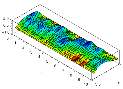
Figure 1: one realisation of the space-time dependence of the stochastic field $w(x,t)$ for parameters $\epsilon\gamma=\sqrt{\epsilon}\sigma=1$ . The stochastically forced $\sin 2x$ mode interacts nonlinearly with the finite amplitude fundamental mode $\sin x$ . The numerics are based on finite differences with $15$ points in space.

6.1 Averaging and deviation

Consider the following stochastic forced heat equation on the domain $[0\,,\pi]$

$$\partial_{t}w=\partial_{xx}w+(1+\epsilon\gamma)w-w^{3}+\sigma\sqrt{\epsilon}\partial_{t}W$$ (49)

with $w(0,t)=w(\pi,t)=0$ . $\gamma$ is a real bifurcation parameter. The spatiotemporal noise $W$ is defined by (12) with $\lambda_{2}=1$ and $\lambda_{i}=0$ for $i\neq 2$ , that is, $W(x,t)=\beta_{2}(t)\sin 2x$ . Then only the second spatial mode is forced by white noise. Figure 1 plots one realisation illustrating the nonlinear dynamics induced by the noise of strength $\sqrt{\epsilon}\sigma$. In the spde (49) we incorporate the growth linear in $w$ to counteract the dissipation on a finite domain so that we can control the clarity of the separation between fast and slow modes. We take $A_{1}=\partial_{xx}+1$ with Dirichlet boundary condition on $[0,\pi]$, then the eigenmodes $e_{i}(x)=\sin(ix)$ corresponding to decay rates $\alpha_{i}=i^{2}-1$ : giving the slow mode $\sin x$ ; and the fast modes $\sin ix$ for $i\geq 2$ . As the parameter $\epsilon\gamma$ crosses zero with no noise, $\sigma=0$, there is a deterministic bifurcation to a finite amplitude of the fundamental mode $\sin x$ .

We consider the stochastic system (49) on long timescales of order $\epsilon^{-1}$ . First notice that here $f(w)=\epsilon w-w^{3}$ , but all the analysis in Section 5 holds. Then decompose the field $w^{\epsilon}(t)=\sqrt{\epsilon}u^{\epsilon}(t^{\prime})+\sqrt{\epsilon}v^{\epsilon}(t^{\prime})$ in the slow time $t^{\prime}=\epsilon t$ . By Theorem 2 the fast mode $v^{\epsilon}$ is approximated by a stationary process $\eta$ which solves the following linear equation for small $\epsilon>0$

$$\partial_{t^{\prime}}\eta=\frac{1}{\epsilon}\partial_{xx}\eta+\frac{\sigma}{\sqrt{\epsilon}}Q_{N}\partial_{t^{\prime}}W\,.$$

Decomposing $\eta=\sum_{i}\eta_{i}e_{i}$, then $\eta_{i}=0$ for $i\neq 2$ and the scalar stationary process $\eta_{2}$ then satisfies the following stochastic ordinary differential equation

$$d\eta_{2}=-\frac{3}{\epsilon}\eta_{2}\,dt^{\prime}+\sigma\sqrt{\frac{1}{\epsilon}}\,d\beta^{\prime}_{2}\,.$$

The distribution of $\eta_{2}$ is the one dimensional normal distribution $\mathcal{N}\big{(}0\,,\frac{1}{6}{\sigma^{2}}\big{)}$.

$\bar{a}^{2}$
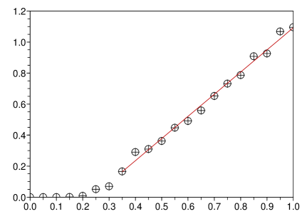
	bifurcation parameter $\epsilon\gamma$

Figure 2: average equilibrium amplitude (squared) of the fundamental mode, $\bar{a}^{2}$, versus bifurcation parameter $\epsilon\gamma$ for fixed noise amplitude $\sqrt{\epsilon}\sigma=1$ . The straight line fit is $\bar{a}^{2}\approx+1.41\epsilon\gamma-0.32$ .

Theorem 2 also asserts that the averaged equation for $u^{\epsilon}$ is

$$\partial_{t^{\prime}}u=\gamma u-\mathcal{P}_{1}u^{3}-\frac{3\sigma^{2}}{6}\mathcal{P}_{1}u\sin^{2}2x\,.$$ (50)

Suppose $u=A(t^{\prime})\sin x$, by (50) the amplitude $A$ satisfies the Landau equation

$$\frac{dA}{dt^{\prime}}=\Big{(}\gamma-\frac{\sigma^{2}}{4}\Big{)}A-\frac{3}{4}A^{3}\,.$$ (51)

Figure 2 plots the average amplitudes, $\bar{a}$, of the fundamental mode obtained from numerical simulations. The figure shows that the amplitude of the fundamental is depressed by the noise in the second component causing a delay in the bifurcation in the presence of noise. More extensive numerical simulations suggest that the mean amplitude depends upon noise and bifurcation parameter (for $0\leq\epsilon\gamma,\epsilon\sigma^{2}<1$) according to

$$\bar{a}^{2}\approx\epsilon\big{(}1.32\,\gamma-0.34\,\sigma^{2}\big{)}+\epsilon^{2}\big{(}0.08\,\gamma^{2}+0.03\,\gamma\sigma^{2}+0.02\,\sigma^{4}\big{)}.$$ (52)

The analytic Landau equation predicts equilibrium amplitude $A^{2}=\frac{4}{3}\gamma-\frac{1}{3}\sigma^{2}$ which (after scaling by $\epsilon$) agrees remarkably well with these numerical estimates.

$a$
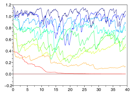
	time $t$

Figure 3: realisations of the amplitude of the fundamental mode $a(t)$ versus time for various bifurcation parameters $\epsilon\gamma$ and for noise amplitude $\sqrt{\epsilon}\sigma=1$ . At time zero the fundamental modes are started at the deterministic stable equilibrium for the corresponding $\epsilon\gamma$.

However, there is also a significant stochastic component in the fundamental mode, $\sin x$ , as shown by Figure 3 which plots the amplitude of the fundamental as a function of time for various bifurcation parameters $\epsilon\gamma$. The stochastic fluctuations come from nonlinear interactions of the noise in the $\sin 2x$ mode. Now we calculate this deviation. Noting that $\eta=\eta_{2}\sin 2x$ , Lemma 6 asserts

$$B(A) = 2\mathbb{E}\int_{0}^{\infty}\big{[}\mathcal{P}_{1}(u+\eta(s))^{3}-\overline{\mathcal{P}_{1}(u+\eta)^{3}}\big{]}\big{[}\mathcal{P}_{1}(u+\eta(0))^{3}-\overline{\mathcal{P}_{1}(u+\eta)^{3}}\big{]}\,ds$$

$$= 18A^{2}\int_{0}^{\infty}\mathbb{E}\Big{[}\big{(}\eta^{2}_{2}(s)-\mathbb{E}\eta^{2}_{2}\big{)}\big{(}\eta^{2}_{2}(0)-\mathbb{E}\eta^{2}_{2}\big{)}\Big{]}\langle e_{1}^{2},e^{2}_{2}\rangle^{2}\,ds$$

$$= \frac{\sigma^{4}}{24}A^{2}\,.$$

Then writing $\lim_{\epsilon\to 0}(u^{\epsilon}-u)/{\sqrt{\epsilon}}:=\rho_{1}\sin x$ , by $3\mathcal{P}_{1}[(\mathbb{E}\eta^{2})\rho_{1}]=\sigma^{2}\rho_{1}/4$ , the deviation $\rho_{1}$ solves the Ornstein–Uhlenbeck-like sde

$$d\rho_{1}=\left(\gamma-\frac{\sigma^{2}}{4}-\frac{9}{4}A^{2}\right)\rho_{1}\,dt+\frac{\sigma^{2}}{2\sqrt{6}}A\,d\beta\,,\quad\rho_{1}(0)=0\,,$$ (53)

where $\beta$ is a standard real valued Brownian motion. For example, after the mean amplitude $A$ reaches equilibrium, $A=\sqrt{4(\gamma-\sigma^{2}/4)/3}$, the sde (53) predicts fluctuations in $\rho_{1}$ with a standard deviation

$$\sigma_{1}\approx\frac{\sigma^{2}}{6\sqrt{2}}=0.1179\,\epsilon\sigma^{2}.$$ (54)

Such fluctuations are seen in the numerical simulations of Figure 3. More extensive numerical simulations estimates the standard deviation of the fluctuations; Figure 4 plots this standard deviation against the noise amplitude. A straight line fit to this data gives the standard deviation of the numerically observed fluctuations as $\sigma_{a}\approx 0.08\,\sigma^{2}$. The theoretical prediction (54) scales the same with applied noise $\sigma$, although the coefficient is about $30\%$ different, and is similarly independent of the bifurcation parameter $\epsilon\gamma$. Averaging and deviation together reasonably predict the dynamics of this example spde (49).

standard deviation $\sigma_{a}$
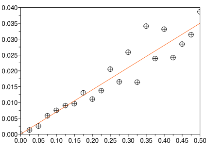
	noise $\epsilon\sigma^{2}$

Figure 4: standard deviation of the amplitude $a(t)$ of the fundamental mode $\sin x$ versus noise $\epsilon\sigma^{2}$ for fixed bifurcation parameter $\epsilon\gamma=1$ . These are estimated from long time versions of the simulations shown in Figure 3. The straight line fit predicts $\sigma_{a}\approx 0.07\epsilon\sigma^{2}$.

6.2 Compare with the stochastic slow manifold

Earlier work constructing stochastic slow manifolds of dissipative spdes [14] is easily adapted to the example spde (49). Recall we choose $W=\beta_{2}(t)\sin 2x$ . In terms of the amplitude $a(t)$ of the fundamental mode $\sin x$ , computer algebra readily derives that the stochastic slow manifold of the spde (49) is

$$w = a\sin x+\frac{1}{32}a^{3}\sin 3x+\sqrt{\epsilon}\sigma\sin 2x\,e^{-3t}\star\dot{\beta}_{2}$$ (55)

$${}+\epsilon^{3/2}\gamma\sigma\sin 2x\,e^{-3t}\star e^{-3t}\star\dot{\beta}_{2}+\cdots\,.$$

The history convolutions of the noise, $e^{-3t}\star\dot{\beta}_{2}=\int_{-\infty}^{t}e^{-3(t-s)}d\beta_{2}(s)$ that appear in the shape of this stochastic slow manifold empower us to eliminate such history integrals in the evolution except in the nonlinear interactions between noises; here simply

$$\dot{a}=\epsilon\gamma a-\frac{3}{4}a^{3}-\frac{1}{2}\epsilon\sigma^{2}a\,\big{(}\dot{\beta}_{2}e^{-3t}\star\dot{\beta}_{2}\big{)}+\cdots\,.$$

Analogously to the averaging and devaition theorems, analysis of Fokker–Planck equations [6, 14] then asserts that the cannonical quadratic noise interaction term in this equation should be replaced by the sum of a mean drift and an effectively new independent noise process. Thus the evolution on this stochastic slow manifold is

$$da\approx\left[\epsilon\left(\gamma-\frac{1}{4}\sigma^{2}\right)a-\frac{3}{4}a^{3}\right]dt+\frac{1}{2\sqrt{6}}\epsilon\sigma^{2}a\,d\tilde{\beta}+\cdots\,,$$ (56)

where $\tilde{\beta}$ is a real valued standard Brownian motion. The stochastic model (56) is exactly the averaged equation (51) plus the deviation (53) with $a(t)=\sqrt{\epsilon}A(\epsilon t)+\epsilon\rho_{1}(\epsilon t)$ . And the stochastic model (52) predicts a stochastic equilibrium amplitude squared of about $\bar{a}^{2}=\frac{4}{3}\epsilon\gamma-\frac{1}{3}\epsilon\sigma^{2}$ in agreement with the empirical fit (52) to the numerical data of Figure 2 and other simulations.

Now investigate the fluctuations about the stochastic equilibrium as seen in Figure 3 and measured in Figure 4. As for the deviation equation (53), the stochastic slow model (56) is approximately an Orstein–Uhlenbeck process in the vicinity of the finite amplitude stochastic equilibrium. Without elaborating the details, the form of (56) then predicts fluctuations about the equilibrium have a standard deviation of $\epsilon\sigma^{2}/(6\sqrt{2})$ in agreement with (54) and in moderate agreement with the fit of Figure 4 to the numerical simulations. The stochastic slow manifold model also predicts the stochastic dynamics of this example spde (49). The difference is that the stochastic slow manifold model is encapsulated in the one sde (56) instead of being split into separate equations for the average and deviation.

Acknowledgements

This research is supported by the Australian Research Council grant DP0774311 and NSFC grant 10701072.

References

- [1] L. Bertini, E. Presutti, B. Rüdiger & E. Saada, Dynamical fluctuations at the critical point: convergence to a non linear stochastic PDE, Theory Probab Appl, 38(1993), 689–741.
- [2] D. Blömker & M. Haire, Amplitude equations for SPDEs: Approximate centre manifolds and invariant measures, Probability and partial differential equations in modern applied mathematics, (Ed. J. Duan & E.C. Waymire), Springer, 2005.
- [3] D. Blömker, M. Haire & G.A. Pavliotis, Multiscale analysis for SPDEs with quadratic nonlinearities, Nonlinearity, 20 (2007), 1721–1744. http://dx.doi.org/10.1088/0951-7715/20/7/009
- [4] D. Blömker, S. Maier-Paape & G. Schneider, The stochastic Landau equation as an amplitude equation, Discrete and Continuous Dynamical Systems, B, 1(4) (2001), 527–541.
- [5] M. F. Chen, From Markov Chains to Non-Equilibrium Particle Systems, World Scientific Publishing, Singapore, 1992.
- [6] Xu Chao and A. J. Roberts, On the low-dimensional modelling of Stratonovich stochastic differential equations, Physica A, 225 (1996) 62–80. http://dx.doi.org/10.1016/0378-4371(95)00387-8
- [7] G. Da Prato & J. Zabczyk, Stochastic Equations in Infinite Dimensions, Cambridge University Press, 1992.
- [8] W. E, X. Li & E. Vanden-Eijnden, Some recent progress in multiscale modeling, Multiscale modelling and simulation, Lect. Notes Comput. Sci. Eng., 39, 3–21, Springer, Berlin, 2004.
- [9] P. Imkeller & A. Monahan (Eds.). Stochastic Climate Dynamics, a Special Issue in the journal Stoch. and Dyna., 2(3), 2002.
- [10] H. Kesten & G. C. Papanicolaou, A limit theorem for turbulent diffusion, Commun. Math. Phys., 65(1979), 79–128. http://dx.doi.org/10.1007/3-540-08853-9_30
- [11] M. Metivier, Stochastic Partial Differential Equations in Infinite Dimensional Spaces, Scuola Normale Superiore, Pisa, 1988.
- [12] G. A. Pavliotis & A. M. Stuart, Multiscale Methods: Averaging and Homogenization, Springer, Berlin, 2007.
- [13] A. J. Roberts, A step towards holistic discretisation of stochastic partial differential equations, In Jagoda Crawford and A. J. Roberts, editors, Proc. of 11th Computational Techniques and Applications Conference CTAC-2003, volume 45 (2003), C1–C15. http://anziamj.austms.org.au/V45/CTAC2003/Robe.
- [14] A. J. Roberts, Resolving the multitude of microscale interactions accurately models stochastic partial differential equations, LMS J. Computation and Maths, 9 (2006), 193–221. http://www.lms.ac.uk/jcm/9/lms2005-032
- [15] A. J. Roberts, Normal form transforms separate slow and fast modes in stochastic dynamical systems, Physica A, 387 (2008) 12–38. http://dx.doi.org/10.1016/j.physa.2007.08.023
- [16] J. Simon, Compact sets in the space , Ann. Mat. Pura Appl., 146 (1987), 65–96. http://dx.doi.org/10.1007/BF01762360
- [17] W. Wang & A. J. Roberts, Average and deviation for slow–fast stochastic partial differential equations, Technical report, 2008.
- [18] H. Watanabe, Averaging and fluctuations for parabolic equations with rapidly oscillating random coefficients, Probab. Th. & Rel. Fields, 77 (1988), 359–378. http://dx.doi.org/10.1007/BF00319294
- [19] S. Engblom, L. Ferm, A. Hellander & P. Lötstedt, Simulation of stochastic reaction diffusion processes on unstructured meshes, Technical report, http://arXiv.org/abs/0804.3288, 2008.