Exact dynamical exchange-correlation kernel of a weakly inhomogeneous electron gas

Abstract

The dynamical exchange-correlation kernel $f_{xc}$ of a non-uniform electron gas is an essential input for the time-dependent density functional theory of electronic systems. The long-wavelength behavior of this kernel is known to be of the form $f_{xc}=\alpha/q^{2}$ where $q$ is the wave vector and $\alpha$ is a frequency-dependent coefficient. We show that in the limit of weak non-uniformity the coefficient $\alpha$ has a simple and exact expression in terms of the ground-state density and the frequency-dependent kernel of a uniform electron gas at the average density. We present an approximate evaluation of this expression for Si and discuss its implications for the theory of excitonic effects.

Since its introduction in works of Runge, Gross, and Kohn Runge and Gross (1984); Gross and Kohn (1985), the time-dependent density-functional theory (TDDFT) has evolved into a powerful tool of investigation of systems ranging from isolated atoms to bulk solids. In the important linear-response regime, the key quantity of TDDFT is the dynamical exchange-correlation (xc) kernel $f_{xc}$ defined as the functional derivative

$$f_{xc}[n_{0}({\bf r})]({\bf r},{\bf r}^{\prime},\omega)=\left.\frac{\delta V_{xc}[n]({\bf r},\omega)}{\delta n({\bf r}^{\prime},\omega)}\right|_{n=n_{0}({\bf r})}$$

of the dynamical exchange and correlation potential $V_{xc}$ with respect to the dynamical electron density $n$, taken at the ground-state value $n_{0}$ of the latter. With this definition, the density-response function $\chi$ can be represented in operator notation as Gross and Kohn (1985)

$$\chi({\bf r},{\bf r}^{\prime},\omega)=\left\{[1-\chi_{KS}(C+f_{xc})]^{-1}\chi_{KS}\right\}({\bf r},{\bf r}^{\prime},\omega)\,,$$ (1)

where $\chi_{KS}$ is the Kohn-Sham (KS) density-response function of independent electrons, $C=e^{2}/|{\bf r}-{\bf r}^{\prime}|$ is the Coulomb interaction, and $e$ is the absolute value of the electron charge. While the density-response function of non-interacting electrons $\chi_{KS}$ can be straightforwardly calculated in many cases of interest (e.g., for homogeneous electron gases in three and two dimensions it is given by the analytical Lindhard’s Lindhard (1954) and Stern’s Stern (1967) formulas, respectively), the construction of $f_{xc}$, whose role is to account for dynamical many-body correlations, is not straightforward.

As an instructive specific case, let us consider the excitonic effect Ashcroft and Mermin (1976) in a semiconductor, which would manifest itself as an enhancement of the imaginary part of $\chi$ for frequencies close to the fundamental absorption edge. We neglect for a moment local-field effects and write down the diagonal elements of the density response in momentum space as of Eq. (1)

$$\chi({\bf q},{\bf q},\omega)=\frac{\chi_{KS}({\bf q},{\bf q},\omega)}{1-\chi_{KS}({\bf q},{\bf q},\omega)[\frac{4\pi e^{2}}{q^{2}}+f_{xc}({\bf q},{\bf q},\omega)]}\,$$ (2)

where $4\pi e^{2}/q^{2}$ is the Fourier transform of the Coulomb interaction. On the one hand, the excitonic enhancement of $\chi$ is a many-body effect and, therefore, it needs a nonzero $f_{xc}$ to be accounted for within TDDFT. On the other hand, because of the divergent Coulomb part $4\pi e^{2}/q^{2}$ in Eq. (2), any $f_{xc}(q,q,\omega)$ that remained finite at $q=0$ would give no contribution in the long-wave limit $q\rightarrow 0$. This simple observation shows that in order to include the exciton, $f_{xc}({\bf q},{\bf q},\omega)$ must be divergent in the long-wave limit at least as strongly as the Coulomb term. And indeed, when the $q^{-2}$ divergence has been introduced empirically in papers dealing with the optical absorption spectrum of semiconductors Reining et al. (2002); Del Sole et al. (2003); Botti et al. (2004), it has yielded a good TDDFT description of the excitonic effect.

Clearly it would be highly desirable to have a first-principle theory of the small-${\bf q}$ behavior of the xc kernel, rather than relying on empirical parametrizations. In this Letter we take a step in this direction. We first show that the asymptotic relation

$$\lim_{{\bf q}\rightarrow 0}f_{xc}({\bf q},{\bf q},\omega)=\frac{e^{2}\alpha(\omega)}{q^{2}}$$ (3)

(we introduce the $e^{2}$ so that $\alpha$ is dimensionless) is a rigorous consequence of exact sum rules for the current density response function. Then, in the limit of weak non-uniformity we obtain a simple and exact expression for $\alpha(\omega)$ in terms of the ground-state density and the dynamical xc kernel of a homogeneous electron gas at the average density.

We start by noting that the local density approximation (LDA) to $f_{xc}$ is unable to produce the divergence. Indeed, within LDA Gross and Kohn (1985)

$$f_{xc}({\bf r},{\bf r}^{\prime},\omega)=f_{xc}^{h}[n({\bf r}),\omega]\,\delta({\bf r}-{\bf r}^{\prime}),$$ (4)

where $f_{xc}^{h}(n,\omega)$ is the long-wave limit of the xc kernel of the homogeneous electron gas of density $n$. The latter is known Gross and Kohn (1985); Nifosì et al. (1998); Conti and Vignale (1999); Qian and Vignale (2002) to be finite, no divergence arising, therefore, in the Fourier transform of Eq. (4).

To obtain an accurate non-local $f_{xc}$, we resort to the recently proposed general method Nazarov et al. (2007) derived from the time-dependent current-density functional theory (TDCDFT) Vignale and Kohn (1996). This method is based on the exact relation that holds between the scalar density-response function $\chi$ (density response to a scalar potential) and the tensor current-density-response function $\hat{\chi}$ (current-density response to a vector potential):

$$\chi({\bf q},{\bf q}^{\prime},\omega)=\frac{c}{e\omega^{2}}{\bf q}\cdot\hat{\chi}({\bf q},{\bf q}^{\prime},\omega)\cdot{\bf q}^{\prime}.$$ (5)

Both response functions are expressed in terms of the corresponding Kohn-Sham response functions and xc kernels in the following manner:

$$\chi^{-1}({\bf q},{\bf q}^{\prime},\omega)=\chi_{KS}^{-1}({\bf q},{\bf q}^{\prime},\omega)-f_{xc}({\bf q},{\bf q}^{\prime},\omega)-\frac{4\pi e^{2}}{q^{2}}\delta_{{\bf q}{\bf q}^{\prime}}$$ (6)

and

$$\hat{\chi}^{-1}({\bf q},{\bf q}^{\prime},\omega)=\hat{\chi}_{KS}^{-1}({\bf q},{\bf q}^{\prime},\omega)-\hat{f}_{xc}({\bf q},{\bf q}^{\prime},\omega)-\frac{4\pi ec}{\omega^{2}}\hat{L}_{{\bf q}}\delta_{{\bf q}{\bf q}^{\prime}}\,,$$ (7)

where $\hat{L}_{{\bf q},ij}\equiv q_{i}q_{j}/q^{2}$, $i$ and $j$ are cartesian indices.

Equations (5-7) establish a connection between $f_{xc}$ and its tensor counterpart $\hat{f}_{xc}$. The usefulness of this connection stems from the fact that the tensor quantities $\hat{\chi}_{KS}$ and $\hat{f}_{xc}$ satisfy a broader set of exact sum rules than the corresponding scalar quantities. These sum rules were derived in Ref. Vignale and Kohn (1998). Specializing to the case of a periodic systems, the two most important sum rules for our purposes are

$$\hat{\chi}_{KS,ij}({\bf G},0,\omega)=\frac{e}{mc}n_{0}({\bf G})\delta_{ij}$$ (8)

$$-\frac{1}{m\omega^{2}}\sum\limits_{{\bf G}^{\prime},k}\hat{\chi}_{KS,i,k}({\bf G},{\bf G}^{\prime},\omega)G^{\prime}_{k}G^{\prime}_{j}V_{KS}({\bf G}^{\prime})\,,$$ (9)

and

$$\sum\limits_{{\bf G}^{\prime}}\hat{f}_{xc,ij}({\bf G},{\bf G}^{\prime},\omega)n_{0}({\bf G}^{\prime})=\frac{c}{e\omega^{2}}\,G_{i}G_{j}V_{xc}({\bf G})\,,$$ (10)

where ${\bf G}$ are reciprocal lattice vectors. These sum rules connect three different types of components of, say, $\chi_{KS}({\bf G},{\bf G}^{\prime},\omega)$: the $({\bf 0},{\bf 0})$ component, the $({\bf 0},{{\bf G}\neq{\bf 0}})$ and $({{\bf G}\neq{\bf 0}},{\bf 0})$ components, and the $({{\bf G}\neq{\bf 0}},{{\bf G}^{\prime}\neq{\bf 0}})$ components.

Let us further restrict our attention to the case of a weakly inhomogeneous system: $|n_{0}({\bf G})|\ll n_{0}({\bf 0})\equiv\bar{n}_{0}$, and $|V_{KS}({\bf G})|\ll\hbar^{2}G^{2}/2m$ for ${\bf G}\neq{\bf 0}$. Then it is easily shown that the homogenous electron gas approximation for the $({{\bf G}\neq{\bf 0}},{{\bf G}^{\prime}\neq{\bf 0}})$ components completely determines the $({\bf 0},{{\bf G}\neq{\bf 0}})$ and $({{\bf G}\neq{\bf 0}},{\bf 0})$ components to first order in $n_{0}({\bf G}\neq{\bf 0})$, which in turn completely determines the $({\bf 0},{\bf 0})$ component to second order in $n_{0}({\bf G}\neq{\bf 0})$. Thus, for $\hat{\chi}_{KS}$ we obtain

$$\hat{\chi}_{KS,ij}({\bf G}\neq{\bf 0},{\bf G}^{\prime}\neq{\bf 0},\omega) = \left[\frac{e\omega^{2}}{c\,G^{2}}L_{{\bf G},ij}\,\chi^{hL}_{KS}(G,\omega)+T_{{\bf G},ij}\,\chi^{hT}_{KS}(G,\omega)\right]\delta_{{\bf GG}^{\prime}}\,,$$ (11)

$$\hat{\chi}_{KS,ij}({\bf G}\neq{\bf 0},{\bf 0},\omega) = \hat{\chi}_{KS,ij}({\bf 0},-{\bf G},\omega)=\frac{e}{mc}\left[n_{0}({\bf G})\delta_{ij}-L_{{\bf G},ij}\chi^{hL}_{KS}(G,\omega)V_{KS}({\bf G})\right]\,,$$ (13)

$$\hat{\chi}_{KS,ij}({\bf 0},{\bf 0},\omega) = \frac{e\bar{n}_{0}}{mc}\delta_{ij}+\frac{e}{m^{2}\omega^{2}c}\sum\limits_{{\bf G}\neq{\bf 0}}G^{2}L_{{\bf G},ij}|V_{KS}({\bf G})|^{2}\left[\chi^{hL}_{KS}(G,\omega)-\chi^{hL}_{KS}(G,0)\right]\,.$$ (15)

to the zero-th, first, and second order in $V_{KS}({\bf G})$, respectively. Here $\chi^{hL}_{KS}$ and$\chi^{hT}_{KS}$ are, respectively, the longitudinal and transverse KS density-response functions of the homogeneous electron gas of density $\bar{n}_{0}$, and $T_{{\bf G},ij}=\delta_{ij}-L_{{\bf G},ij}$. Similarly, for $\hat{f}_{xc}$ we have

$$\hat{f}_{xc,ij}({\bf G}\neq 0,{\bf G}^{\prime}\neq 0,\omega)=\frac{c}{e\omega^{2}}\,G^{2}\!\left[f_{xc}^{hL}(G,\omega)L_{{\bf G},ij}\!+\!f_{xc}^{hT}(G,\omega)T_{{\bf G},ij}\right]\delta_{{\bf GG}^{\prime}}\,,$$

$$\hat{f}_{xc,ij}({\bf G}\neq{\bf 0},{\bf 0},\omega)\!=\!\hat{f}_{xc,ji}({\bf 0},-{\bf G},\omega)\!=\!-\frac{c\,G^{2}}{e\omega^{2}\bar{n}_{0}}n_{0}({\bf G})\!\left\{[f_{xc}^{hL}(G,\omega)\!-\!f_{xc}^{hL}(G,0)]L_{{\bf G},ij}\!+\!f_{xc}^{hT}(G,\omega)T_{{\bf G},ij}\!\right\}\,,$$

$$\hat{f}_{xc,ij}({\bf 0},{\bf 0},\omega)=\frac{c}{e\omega^{2}\bar{n}_{0}^{2}}\sum\limits_{{\bf G}\neq{\bf 0}}G^{2}|n_{0}({\bf G})|^{2}\left\{\left[f_{xc}^{hL}(G,\omega)-f_{xc}^{hL}(G,0)\right]L_{{\bf G},ij}+f_{xc}^{hT}(G,\omega)T_{{\bf G},ij}\right\},$$ (16)

where $f_{xc}^{hL}$ and $f_{xc}^{hT}$ are the longitudinal and transverse, respectively, xc kernels of the homogeneous electron gas of density $\bar{n}_{0}$.

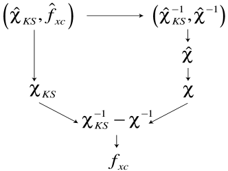
Figure 1: Scheme of the procedure for calculating the xc kernel $f_{xc}$ starting from the expressions (15) and (16) for $\hat{\chi}_{KS}$ and $\hat{f}_{xc}$, respectively.

The following steps, which involve repeated inversions of infinite matrices, rely on the mathematical fact that to find the $({\bf 0},{\bf 0})$, $({\bf 0},{\bf G}\neq{\bf 0})/({\bf G}\neq{\bf 0},{\bf 0})$, and $({\bf G}\neq{\bf 0},{\bf G}^{\prime}\neq{\bf 0})$ elements of the inverse matrix to the second, first, and zeroth order in the inhomogeneity, respectively, it is sufficient to know the corresponding elements of the original matrix to the same accuracy, and then the inversion can be performed in a closed form Sturm (1982).

The complete procedure is schematically illustrated in Fig. (1). Starting from Eqs. (15) and (16) for $\hat{\chi}_{KS}$ and $\hat{f}_{xc}$ we (i) Invert Eqs. (15) to get $\hat{\chi}_{KS}^{-1}$; (ii) Combine $\hat{\chi}_{KS}^{-1}$ and $\hat{f}_{xc}$ to get $\hat{\chi}^{-1}$ by virtue of Eq. (7); (iii) Invert $\hat{\chi}^{-1}$ to get $\hat{\chi}$ ; (iv) Use Eq. (5) and its KS analogue to find the scalar response function $\chi$ from $\hat{\chi}$ and $\chi_{KS}$ from $\hat{\chi}_{KS}$; (v) Invert $\chi$ and $\chi_{KS}$ to get $\chi^{-1}$ and $\chi_{KS}^{-1}$; and, (vi) Apply Eq. (7) to find $f_{xc}$. The final result of this procedure is

$$\lim_{q\rightarrow 0}f_{xc}({\bf G}\neq{\bf 0},{\bf G}^{\prime}\neq{\bf 0},\omega)=f^{h}_{xc,L}(G,\omega)\delta_{{\bf GG}^{\prime}},$$ (17)

$$\lim_{q\rightarrow 0}f_{xc}({\bf G}\neq{\bf 0},{\bf q},\omega)=f_{xc}(-{\bf q},-{\bf G},\omega)=-\frac{({\bf G}\cdot{\hat{\bf q}})}{\bar{n}_{0}q}\left[f_{xc}^{hL}(G,\omega)-f_{xc}^{hL}(G,0)\right]n_{0}({\bf G}),$$ (18)

$$\lim_{q\rightarrow 0}f_{xc}({\bf q},{\bf q},\omega)=\frac{1}{\bar{n}_{0}^{2}q^{2}}\sum\limits_{{\bf G}\neq{\bf 0}}({\bf G}\cdot{\hat{\bf q}})^{2}\left[f_{xc}^{hL}(G,\omega)-f_{xc}^{hL}(G,0)\right]|n_{0}({\bf G})|^{2},$$ (19)

where $\hat{\bf q}$ is the unit vector parallel to ${\bf q}$. It should be noted at this point that the above expression for the scalar kernel $f_{xc}({\bf q},{\bf q},\omega)$ differs from what one would get by simply taking the longitudinal component of $\hat{f}_{xc,ij}({\bf q},{\bf q},\omega)$, i.e. $f_{xc}({\bf q},{\bf q},\omega)\neq\frac{e\omega^{2}}{cq^{2}}\sum_{i,j}\hat{q}_{i}\hat{f}_{xc,ij}({\bf q},{\bf q},\omega)\hat{q}_{j}$. The implication is that the scalar xc potential ($V_{xc}$) of time-dependent DFT is not equivalent to the longitudinal component of the vector potential (${\bf A}_{xc}$) of time-dependent CDFT: rather, it should be constructed through the careful inversion procedure described above. A recent interesting attempt to construct $V_{xc}$ from ${\bf A}_{xc}$ Maitra and van Faassen (2007) should be re-examined in the light of this result.

From the result of the step (iv) for $\chi$ and making use of the relation

$$\frac{1}{\epsilon_{M}(\omega)}=1+\lim_{q\rightarrow 0}\frac{4\pi e^{2}}{q^{2}}\chi({\bf q},{\bf q},\omega),$$ (20)

we obtain a formula for the macroscopic dielectric function of a crystal

$$\!\!\!\!\!\!\!\!\!\!\!\epsilon_{M}(\omega)=1-\frac{4\pi e^{2}\bar{n}_{0}}{m\omega^{2}}-\frac{e^{2}}{m^{2}\omega^{4}}$$ (21)

(22)

$$\!\!\!\!\!\!\!\!\!\!\!\!\!\!\!\times\sum\limits_{{\bf G}\neq 0}|V_{0}({\bf G})|^{2}G^{2}(\hat{{\bf q}}\cdot{\bf G})^{2}\left[\frac{1}{\epsilon^{hL}(G,\omega)}-\frac{1}{\epsilon^{hL}(G,0)}\right]\!\!,$$ (23)

where $V_{0}$ is the bare crystalline potential and

$$\epsilon^{hL}(q,\omega)=1-\frac{4\pi e^{2}}{q^{2}}\frac{\chi^{hL}_{KS}(q,\omega)}{1-\chi^{hL}_{KS}(q,\omega)f^{h}_{xc,L}(q,\omega)}$$

is the longitudinal dielectric function of the homogeneous electron liquid. Equation (23) is in agreement with the Hopfield’s formula for optical conductivity Hopfield (1965), while in the RPA [$f^{h}_{xc,L}(G,\omega)=0$] it coincides with the corresponding result of Ref. Sturm, 1982.

Equations (17-19) are the main result of this paper. They replace the grossly inaccurate LDA formula

$$\lim_{q\rightarrow 0}f_{xc}({\bf G}+{\bf q},{\bf G}^{\prime}+{\bf q},\omega)=f^{h}_{xc,L}(G,\omega)\delta_{{\bf GG}^{\prime}},$$ (24)

which does not contain the singularity in $q$. Identifying the (${\bf 0},{\bf 0}$) element of the microscopic matrix of the xc kernel in Eqs. (19) as the averaged $f_{xc}$, we see that $f_{xc}$ diverges for $q\rightarrow 0$ as described by Eq. (3), wherein $\alpha(\omega)$ is given by

$$\alpha(\omega)\!\!=\!\!\!\!\sum\limits_{{\bf G}\neq 0}\!\!\!\frac{({\bf G}\!\cdot\!\hat{{\bf q}})^{2}}{\bar{n}_{0}^{2}}\!\left[f_{xc}^{hL}(G,\omega)\!-\!\!f_{xc}^{hL}(G,0)\!\right]\!|n_{0}({\bf G})|^{2}.$$ (25)

Notice that $\alpha(\omega)=0$ in the uniform limit and $\alpha(0)=0$ up to second order in $n_{0}({\bf G}\neq{\bf 0})$ .

In order to calculate $\alpha(\omega)$ from Eq. (25) we need the Fourier amplitudes of the ground-state electron density and the wave vector and frequency-dependent $f_{xc}^{hL}$ of the homogeneous electron gas, evaluated at reciprocal lattice vectors. The first ingredient is straightforwardly obtained from standard electronic structure calculations. Unfortunately, the same cannot be said of the second ingredient $f_{xc}^{hL}(q,\omega)$, for which we do not have reliable expressions. The best that can be done, at this time, is either to disregard the wave vector dependence, or to make use of the interpolation formula proposed in Ref. Dabrowski, 1986, which however fails to reproduce, at small $q$, what is presently believed to be the qualitatively correct form of the frequency dependence. In spite of these difficulties, it must be emphasized that the calculation of $f_{xc}^{hL}(q,\omega)$ is still a much simpler problem than the calculation of the dynamical xc kernel of the non-uniform system. Thus, our Eq. (25) does not simply express an unknown quantity in terms of another unknown quantity, but actually opens the way to systematic calculations of $\alpha$ based on the many-body theory of the homogeneous electron gas. Further, Eqs. (17)-(19) for $f_{xc}$ offer a promising alternative to the widespread practice of treating the dynamical exchange and correlations effects in the LDA.

In Fig. 2 we plot $\alpha(\omega)$ from Eq. (25) vs frequency for crystalline silicon. The Fourier coefficients of the electron density were calculated with the code FHI98MD Bockstedte et al. (1997), and we approximated $f_{xc}^{hL}(q,\omega)\simeq f_{xc}^{hL}(0,\omega)$, taking the latter from Ref. Qian and Vignale, 2002. In the range 0-22 eV, the real part of $\alpha(\omega)$ is negative, changing sign for positive above 22 eV. It reaches its minimum of $\alpha\approx$ -0.1 at $\omega\approx$ 14 eV. In the range 3-5 eV of the main absorption in silicon, ${\rm Re}\,\alpha$ changes from -0.01 to -0.03, which is an order of magnitude smaller than the empirical value of $\alpha\approx$ -0.2 found as the best fit to the experimental spectrum in Ref. Reining et al., 2002. This large difference may simply indicate that the nearly free electron model, while being adequate for simple metals and even for semiconductors in the high-frequency regime Sturm (1982), is not sufficiently accurate for semiconductors at frequency lower than or comparable to the band gap (see also footnote [2]). Another probable source of discrepancy is that our approach is a pure TDDFT, whereas the value of $\alpha\approx-0.2$ was obtained in Refs. Reining et al., 2002 and Del Sole et al., 2003 with the use of self-energies incorporated in the Green’s function via the $GW$ approximation.

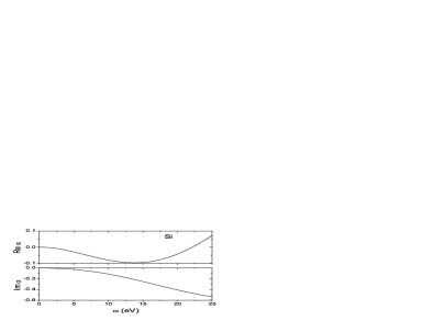
Figure 2: The frequency dependence of the real (upper panel) and image (lower panel) parts of the $\alpha$ coefficient in Eq. (3) for silicon calculated by Eq. (25).

In conclusion, within the nearly free electron approximation, we have constructed the otherwise exact exchange-correlation kernel for time-dependent density-functional theory. This kernel is nonlocal in space, exhibiting the $q^{-2}$ singularity in the reciprocal space. The strength of this singularity, which is frequency-dependent, has been directly related to the magnitude of the non-uniformity of the density of valence electrons, and this singularity disappears in the limiting case of the homogeneous electron liquid. We are proposing an improvement over the conventional LDA scheme of including the dynamical exchange and correlation effects into ab initio calculations of the linear response of crystalline solids which consistently accounts for the long-wave divergence in the exchange-correlation kernel.

GV acknowledges support from DOE Award No. DE-FG02-05ER46203.

References

Runge and Gross (1984)
E. Runge and
E. K. U. Gross,
Phys. Rev. Lett. 52,
997 (1984).
Gross and Kohn (1985)
E. K. U. Gross and
W. Kohn,
Phys. Rev. Lett. 55,
2850 (1985).
Lindhard (1954)
J. Lindhard,
K. Dan. Vidensk. Selsk. Mat.-Fys. Medd.
28, 1 (1954).
Stern (1967)
F. Stern,
Phys. Rev. Lett. 18,
546 (1967).
Ashcroft and Mermin (1976)
N. W. Ashcroft and
N. D. Mermin,
Solid State Physics (Holt,
Rinehart and Winston, New-York, 1976).
Reining et al. (2002)
L. Reining,
V. Olevano,
A. Rubio, and
G. Onida,
Phys. Rev. Lett. 88,
066404 (2002).
Del Sole et al. (2003)
R. Del Sole,
G. Adragna,
V. Olevano, and
L. Reining,
Phys. Rev. B 67,
045207 (2003).
Botti et al. (2004)
S. Botti,
F. Sottile,
N. Vast,
V. Olevano,
L. Reining,
H.-C. Weissker,
A. Rubio,
G. Onida,
R. Del Sole, and
R. W. Godby,
Phys. Rev. B 69,
155112 (2004).
Nifosì et al. (1998)
R. Nifosì,
S. Conti, and
M. P. Tosi,
Phys. Rev. B 58,
12758 (1998).
Conti and Vignale (1999)
S. Conti and
G. Vignale,
Phys. Rev. B 60,
7966 (1999).
Qian and Vignale (2002)
Z. Qian and
G. Vignale,
Phys. Rev. B 65,
235121 (2002).
Nazarov et al. (2007)
V. U. Nazarov,
J. M. Pitarke,
Y. Takada,
G. Vignale, and
Y.-C. Chang,
Phys. Rev. B 76,
205103 (2007).
Vignale and Kohn (1996)
G. Vignale and
W. Kohn,
Phys. Rev. Lett. 77,
2037 (1996).
Vignale and Kohn (1998)
G. Vignale and
W. Kohn, in
Electronic Density Functional Theory: Recent
Progress and New Directions, edited by
J. Dobson,
M. P. Das, and
G. Vignale
(Plenum Press, New York, 1998).
Sturm (1982)
K. Sturm, Adv.
Phys. 31, 1
(1982).
Maitra and van Faassen (2007)
N. T. Maitra and
M. van Faassen,
J. Chem. Phys. 126,
191106 (2007).
Hopfield (1965)
J. J. Hopfield,
Phys. Rev. 139,
A419 (1965).
Dabrowski (1986)
B. Dabrowski,
Phys. Rev. B 34,
4989 (1986).
Bockstedte et al. (1997)
M. Bockstedte,
A. Kley,
J. Neugebauer,
and
M. Scheffler,
Comp. Phys. Comm. 107,
187 (1997), code FHI98MD is
available at http://www.fhi-berlin.mpg.de/th/fhi98md/.