1. Decay amplitudes of B → f 0 ( 980 ) ( π , η ( ′ ) ) → 𝐵 subscript 𝑓 0 980 𝜋 superscript 𝜂 ′ B\to f_{0}(980)(\pi,\eta^{(\prime)})
At present we still do not have a clear understanding about the inner structure
of the scalar mesons.
There are many interpretations for the scalar mesons, such as q q q ¯ q ¯ 𝑞 𝑞 ¯ 𝑞 ¯ 𝑞 qq\bar{q}\bar{q} jaffe q q ¯ 𝑞 ¯ 𝑞 q\bar{q} nato K K ¯ 𝐾 ¯ 𝐾 K\bar{K} jwei
In the four-quark model, the flavor wave function of f 0 ( 980 ) subscript 𝑓 0 980 f_{0}{(980)} jaffe f 0 = s s ¯ ( u u ¯ + d d ¯ ) / 2 subscript 𝑓 0 𝑠 ¯ 𝑠 𝑢 ¯ 𝑢 𝑑 ¯ 𝑑 2 f_{0}=s\bar{s}(u\bar{u}+d\bar{d})/\sqrt{2} f 0 ( 980 ) subscript 𝑓 0 980 f_{0}(980) a 0 ( 980 ) subscript 𝑎 0 980 a_{0}(980) f 0 ( 980 ) subscript 𝑓 0 980 f_{0}(980) a 0 ( 980 ) subscript 𝑎 0 980 a_{0}(980) K K ¯ 𝐾 ¯ 𝐾 K\bar{K} f 0 ( 980 ) subscript 𝑓 0 980 f_{0}(980) hycheng1
In the naive 2-quark model, f 0 ( 980 ) subscript 𝑓 0 980 f_{0}{(980)} s s ¯ 𝑠 ¯ 𝑠 s\bar{s} D s + → f 0 π + → subscript superscript 𝐷 𝑠 subscript 𝑓 0 superscript 𝜋 D^{+}_{s}\to f_{0}\pi^{+} ϕ → f 0 γ → italic-ϕ subscript 𝑓 0 𝛾 \phi\to f_{0}\gamma Γ ( J / ψ → f 0 ω ) ≈ 1 2 Γ ( J / ψ → f 0 ϕ ) Γ → 𝐽 𝜓 subscript 𝑓 0 𝜔 1 2 Γ → 𝐽 𝜓 subscript 𝑓 0 italic-ϕ \Gamma(J/\psi\to f_{0}\omega)\approx\frac{1}{2}\Gamma(J/\psi\to f_{0}\phi) f 0 ( 980 ) → π π → subscript 𝑓 0 980 𝜋 𝜋 f_{0}(980)\to\pi\pi a 0 ( 980 ) → π η → subscript 𝑎 0 980 𝜋 𝜂 a_{0}(980)\to\pi\eta f 0 ( 980 ) subscript 𝑓 0 980 f_{0}{(980)} s s ¯ 𝑠 ¯ 𝑠 s\bar{s} s s ¯ 𝑠 ¯ 𝑠 s\bar{s} n n ¯ ≡ ( u u ¯ + d d ¯ ) / 2 𝑛 ¯ 𝑛 𝑢 ¯ 𝑢 𝑑 ¯ 𝑑 2 n\bar{n}\equiv(u\bar{u}+d\bar{d})/\sqrt{2}
| f 0 ( 980 ) ⟩ = | s s ¯ ⟩ cos θ + | n n ¯ ⟩ sin θ , ket subscript 𝑓 0 980 ket 𝑠 ¯ 𝑠 𝜃 ket 𝑛 ¯ 𝑛 𝜃 \displaystyle|f_{0}(980)\rangle=|s\bar{s}\rangle\cos\theta+|n\bar{n}\rangle\sin\theta, (1)
where θ 𝜃 \theta hycheng2 θ 𝜃 \theta 25 ∘ < θ < 40 ∘ superscript 25 𝜃 superscript 40 25^{\circ}<\theta<40^{\circ} 140 ∘ < θ < 165 ∘ superscript 140 𝜃 superscript 165 140^{\circ}<\theta<165^{\circ} q q ¯ 𝑞 ¯ 𝑞 q\bar{q} duds ; lucd f 0 ( 980 ) subscript 𝑓 0 980 f_{0}(980) s s ¯ 𝑠 ¯ 𝑠 s\bar{s} n n ¯ 𝑛 ¯ 𝑛 n\bar{n}
In the two-quark model, the decay constants for scalar meson f 0 ( 980 ) subscript 𝑓 0 980 f_{0}(980)
⟨ f 0 ( p ) | q ¯ 2 γ μ q 1 | 0 ⟩ quantum-operator-product subscript 𝑓 0 𝑝 subscript ¯ 𝑞 2 subscript 𝛾 𝜇 subscript 𝑞 1 0 \displaystyle\langle f_{0}(p)|\bar{q}_{2}\gamma_{\mu}q_{1}|0\rangle = \displaystyle= 0 , ⟨ f 0 ( p ) | q ¯ 2 q 1 | 0 ⟩ = m S f S ¯ . 0 quantum-operator-product subscript 𝑓 0 𝑝 subscript ¯ 𝑞 2 subscript 𝑞 1 0
subscript 𝑚 𝑆 ¯ subscript 𝑓 𝑆 \displaystyle 0,\quad\langle f_{0}(p)|\bar{q}_{2}q_{1}|0\rangle=m_{S}\bar{f_{S}}. (2)
and
⟨ f 0 n | d ¯ d | 0 ⟩ = ⟨ f 0 n | u ¯ u | 0 ⟩ = 1 2 m f 0 f ~ f 0 n , ⟨ f 0 s | s ¯ s | 0 ⟩ = m f 0 f ~ f 0 s , formulae-sequence quantum-operator-product superscript subscript 𝑓 0 𝑛 ¯ 𝑑 𝑑 0 quantum-operator-product superscript subscript 𝑓 0 𝑛 ¯ 𝑢 𝑢 0 1 2 subscript 𝑚 subscript 𝑓 0 subscript superscript ~ 𝑓 𝑛 subscript 𝑓 0 quantum-operator-product superscript subscript 𝑓 0 𝑠 ¯ 𝑠 𝑠 0 subscript 𝑚 subscript 𝑓 0 subscript superscript ~ 𝑓 𝑠 subscript 𝑓 0 \displaystyle\langle f_{0}^{n}|\bar{d}d|0\rangle=\langle f_{0}^{n}|\bar{u}u|0\rangle=\frac{1}{\sqrt{2}}m_{f_{0}}\tilde{f}^{n}_{f_{0}},\quad\langle f_{0}^{s}|\bar{s}s|0\rangle=m_{f_{0}}\tilde{f}^{s}_{f_{0}}, (3)
where f 0 n superscript subscript 𝑓 0 𝑛 f_{0}^{n} f 0 s superscript subscript 𝑓 0 𝑠 f_{0}^{s} f 0 ( 980 ) subscript 𝑓 0 980 f_{0}(980) f f 0 n superscript subscript 𝑓 subscript 𝑓 0 𝑛 f_{f_{0}}^{n} f f 0 s superscript subscript 𝑓 subscript 𝑓 0 𝑠 f_{f_{0}}^{s} cyf0k ; hycheng1 f ~ f 0 n = f ~ f 0 s superscript subscript ~ 𝑓 subscript 𝑓 0 𝑛 superscript subscript ~ 𝑓 subscript 𝑓 0 𝑠 \tilde{f}_{f_{0}}^{n}=\tilde{f}_{f_{0}}^{s} f ¯ f 0 subscript ¯ 𝑓 subscript 𝑓 0 \bar{f}_{f_{0}}
The twist-2 and twist-3 light-cone distribution amplitudes (LCDAs) for different
components of scalar meson f 0 ( 980 ) subscript 𝑓 0 980 f_{0}(980)
⟨ f 0 ( p ) | q ¯ ( z ) l q ( 0 ) j | 0 ⟩ quantum-operator-product subscript 𝑓 0 𝑝 ¯ 𝑞 subscript 𝑧 𝑙 𝑞 subscript 0 𝑗 0 \displaystyle\langle f_{0}(p)|\bar{q}(z)_{l}q(0)_{j}|0\rangle = \displaystyle= 1 2 N c ∫ 0 1 𝑑 x e i x p ⋅ z 1 2 subscript 𝑁 𝑐 subscript superscript 1 0 differential-d 𝑥 superscript 𝑒 ⋅ 𝑖 𝑥 𝑝 𝑧 \displaystyle\frac{1}{\sqrt{2N_{c}}}\int^{1}_{0}dxe^{ixp\cdot z} (4)
⋅ { p / Φ f 0 ( x ) + m f 0 Φ f 0 S ( x ) + m f 0 ( n / + n / − − 1 ) Φ f 0 T ( x ) } j l . \displaystyle\cdot\left\{p\!\!\!/\Phi_{f_{0}}(x)+m_{f_{0}}\Phi^{S}_{f_{0}}(x)+m_{f_{0}}(n\!\!\!/_{+}n\!\!\!/_{-}-1)\Phi^{T}_{f_{0}}(x)\right\}_{jl}.
Here we assume that f 0 n ( p ) superscript subscript 𝑓 0 𝑛 𝑝 f_{0}^{n}(p) f 0 s ( p ) superscript subscript 𝑓 0 𝑠 𝑝 f_{0}^{s}(p) f 0 ( p ) subscript 𝑓 0 𝑝 f_{0}(p) n + = ( 1 , 0 , 0 T ) subscript 𝑛 1 0 subscript 0 𝑇 n_{+}=(1,0,0_{T}) n − = ( 0 , 1 , 0 T ) subscript 𝑛 0 1 subscript 0 𝑇 n_{-}=(0,1,0_{T})
The twist-2 LCDA Φ f ( x , μ ) subscript Φ 𝑓 𝑥 𝜇 \Phi_{f}(x,\mu)
Φ f ( x , μ ) subscript Φ 𝑓 𝑥 𝜇 \displaystyle\Phi_{f}(x,\mu) = \displaystyle= 1 2 2 N c f ¯ f ( μ ) 6 x ( 1 − x ) ∑ m = 1 ∞ B m ( μ ) C m 3 / 2 ( 2 x − 1 ) , 1 2 2 subscript 𝑁 𝑐 subscript ¯ 𝑓 𝑓 𝜇 6 𝑥 1 𝑥 superscript subscript 𝑚 1 subscript 𝐵 𝑚 𝜇 subscript superscript 𝐶 3 2 𝑚 2 𝑥 1 \displaystyle\frac{1}{2\sqrt{2N_{c}}}\bar{f}_{f}(\mu)6x(1-x)\sum_{m=1}^{\infty}B_{m}(\mu)C^{3/2}_{m}(2x-1), (5)
where the values for Gegenbauer moments are taken at scale μ = 1 GeV 𝜇 1 GeV \mu=1\mbox{GeV} B 1 = − 0.78 ± 0.08 subscript 𝐵 1 plus-or-minus 0.78 0.08 B_{1}=-0.78\pm 0.08 B 2 = 0 subscript 𝐵 2 0 B_{2}=0 B 3 = 0.02 ± 0.07 subscript 𝐵 3 plus-or-minus 0.02 0.07 B_{3}=0.02\pm 0.07
As for the twist-3 distribution amplitudes Φ f s superscript subscript Φ 𝑓 𝑠 \Phi_{f}^{s} Φ f T superscript subscript Φ 𝑓 𝑇 \Phi_{f}^{T}
Φ f S subscript superscript Φ 𝑆 𝑓 \displaystyle\Phi^{S}_{f} = \displaystyle= 1 2 2 N c f ¯ f , Φ f T = 1 2 2 N c f ¯ f ( 1 − 2 x ) . 1 2 2 subscript 𝑁 𝑐 subscript ¯ 𝑓 𝑓 superscript subscript Φ 𝑓 𝑇
1 2 2 subscript 𝑁 𝑐 subscript ¯ 𝑓 𝑓 1 2 𝑥 \displaystyle\frac{1}{2\sqrt{2N_{c}}}\bar{f}_{f},\,\,\,\,\,\,\,\Phi_{f}^{T}=\frac{1}{2\sqrt{2N_{c}}}\bar{f}_{f}(1-2x). (6)
The B meson is treated as a heavy-light system. We here use the same B meson wave
function as in Ref. liu06 ; guodq07 η − η ′ 𝜂 superscript 𝜂 ′ \eta-\eta^{\prime} η q = ( u u ¯ + d d ¯ ) / 2 subscript 𝜂 𝑞 𝑢 ¯ 𝑢 𝑑 ¯ 𝑑 2 \eta_{q}=(u\bar{u}+d\bar{d})/\sqrt{2} η s = s s ¯ subscript 𝜂 𝑠 𝑠 ¯ 𝑠 \eta_{s}=s\bar{s} ϕ η q , s A , P , T superscript subscript italic-ϕ subscript 𝜂 𝑞 𝑠
𝐴 𝑃 𝑇
\phi_{\eta_{q,s}}^{A,P,T} f q = ( 1.07 ± 0.02 ) f π subscript 𝑓 𝑞 plus-or-minus 1.07 0.02 subscript 𝑓 𝜋 f_{q}=(1.07\pm 0.02)f_{\pi} f s = ( 1.34 ± 0.06 ) f π subscript 𝑓 𝑠 plus-or-minus 1.34 0.06 subscript 𝑓 𝜋 f_{s}=(1.34\pm 0.06)f_{\pi} ϕ = 39.3 ∘ ± 1.0 ∘ , e t c italic-ϕ plus-or-minus superscript 39.3 superscript 1.0 𝑒 𝑡 𝑐
\phi=39.3^{\circ}\pm 1.0^{\circ},etc feldmann liu06 ; guodq07 ; ligluon η ( ′ ) superscript 𝜂 ′ \eta^{(\prime)} η 𝜂 \eta η ′ superscript 𝜂 ′ \eta^{\prime}
The pQCD factorization approach has been used to study the B → f 0 ( 980 ) K → 𝐵 subscript 𝑓 0 980 𝐾 B\to f_{0}(980)K chenf0k1 ; wwang wwang B → f 0 ( 980 ) π → 𝐵 subscript 𝑓 0 980 𝜋 B\to f_{0}(980)\pi f 0 ( 980 ) η ( ′ ) subscript 𝑓 0 980 superscript 𝜂 ′ f_{0}(980)\eta^{(\prime)}
Since the b quark is rather heavy we consider the B 𝐵 B B 𝐵 B
P B = M B 2 ( 1 , 1 , 𝟎 T ) , P 2 = M B 2 ( 1 , 0 , 𝟎 T ) , P 3 = M B 2 ( 0 , 1 , 𝟎 T ) , formulae-sequence subscript 𝑃 𝐵 subscript 𝑀 𝐵 2 1 1 subscript 0 𝑇 formulae-sequence subscript 𝑃 2 subscript 𝑀 𝐵 2 1 0 subscript 0 𝑇 subscript 𝑃 3 subscript 𝑀 𝐵 2 0 1 subscript 0 𝑇 \displaystyle P_{B}=\frac{M_{B}}{\sqrt{2}}(1,1,{\bf 0}_{T}),\quad P_{2}=\frac{M_{B}}{\sqrt{2}}(1,0,{\bf 0}_{T}),\quad P_{3}=\frac{M_{B}}{\sqrt{2}}(0,1,{\bf 0}_{T}), (7)
where the meson masses
have been neglected. Putting the anti- quark momenta in B 𝐵 B P 𝑃 P S 𝑆 S k 1 subscript 𝑘 1 k_{1} k 2 subscript 𝑘 2 k_{2} k 3 subscript 𝑘 3 k_{3}
k 1 = ( x 1 P 1 + , 0 , 𝐤 1 T ) , k 2 = ( x 2 P 2 + , 0 , 𝐤 2 T ) , k 3 = ( 0 , x 3 P 3 − , 𝐤 3 T ) . formulae-sequence subscript 𝑘 1 subscript 𝑥 1 superscript subscript 𝑃 1 0 subscript 𝐤 1 𝑇 formulae-sequence subscript 𝑘 2 subscript 𝑥 2 superscript subscript 𝑃 2 0 subscript 𝐤 2 𝑇 subscript 𝑘 3 0 subscript 𝑥 3 superscript subscript 𝑃 3 subscript 𝐤 3 𝑇 \displaystyle k_{1}=(x_{1}P_{1}^{+},0,{\bf k}_{1T}),\quad k_{2}=(x_{2}P_{2}^{+},0,{\bf k}_{2T}),\quad k_{3}=(0,x_{3}P_{3}^{-},{\bf k}_{3T}). (8)
In the pQCD approach, the decay amplitude 𝒜 ( B → P f 0 ) 𝒜 → 𝐵 𝑃 subscript 𝑓 0 {\cal A}(B\to Pf_{0})
𝒜 ( B → P f 0 ) 𝒜 → 𝐵 𝑃 subscript 𝑓 0 \displaystyle{\cal A}(B\to Pf_{0}) ∼ similar-to \displaystyle\sim ∫ d 4 k 1 d 4 k 2 d 4 k 3 Tr [ C ( t ) Φ B ( k 1 ) Φ P ( k 2 ) Φ f 0 ( k 3 ) H ( k 1 , k 2 , k 3 , t ) ] , superscript 𝑑 4 subscript 𝑘 1 superscript 𝑑 4 subscript 𝑘 2 superscript 𝑑 4 subscript 𝑘 3 Tr delimited-[] 𝐶 𝑡 subscript Φ 𝐵 subscript 𝑘 1 subscript Φ 𝑃 subscript 𝑘 2 subscript Φ subscript 𝑓 0 subscript 𝑘 3 𝐻 subscript 𝑘 1 subscript 𝑘 2 subscript 𝑘 3 𝑡 \displaystyle\int\!\!d^{4}k_{1}d^{4}k_{2}d^{4}k_{3}\ \mathrm{Tr}\left[C(t)\Phi_{B}(k_{1})\Phi_{P}(k_{2})\Phi_{f_{0}}(k_{3})H(k_{1},k_{2},k_{3},t)\right], (9)
∼ similar-to \displaystyle\sim ∫ 𝑑 x 1 𝑑 x 2 𝑑 x 3 b 1 𝑑 b 1 b 2 𝑑 b 2 b 3 𝑑 b 3 differential-d subscript 𝑥 1 differential-d subscript 𝑥 2 differential-d subscript 𝑥 3 subscript 𝑏 1 differential-d subscript 𝑏 1 subscript 𝑏 2 differential-d subscript 𝑏 2 subscript 𝑏 3 differential-d subscript 𝑏 3 \displaystyle\int\!\!dx_{1}dx_{2}dx_{3}b_{1}db_{1}b_{2}db_{2}b_{3}db_{3}
⋅ Tr [ C ( t ) Φ B ( x 1 , b 1 ) Φ P ( x 2 , b 2 ) Φ f 0 ( x 3 , b 3 ) H ( x i , b i , t ) S t ( x i ) e − S ( t ) ] , ⋅ absent Tr delimited-[] 𝐶 𝑡 subscript Φ 𝐵 subscript 𝑥 1 subscript 𝑏 1 subscript Φ 𝑃 subscript 𝑥 2 subscript 𝑏 2 subscript Φ subscript 𝑓 0 subscript 𝑥 3 subscript 𝑏 3 𝐻 subscript 𝑥 𝑖 subscript 𝑏 𝑖 𝑡 subscript 𝑆 𝑡 subscript 𝑥 𝑖 superscript 𝑒 𝑆 𝑡 \displaystyle\cdot\mathrm{Tr}\left[C(t)\Phi_{B}(x_{1},b_{1})\Phi_{P}(x_{2},b_{2})\Phi_{f_{0}}(x_{3},b_{3})H(x_{i},b_{i},t)S_{t}(x_{i})\,e^{-S(t)}\right],\quad
where the term “Tr Tr \mathrm{Tr} C ( t ) 𝐶 𝑡 C(t) H ( x i , b i , t ) 𝐻 subscript 𝑥 𝑖 subscript 𝑏 𝑖 𝑡 H(x_{i},b_{i},t) b i subscript 𝑏 𝑖 b_{i} k i T subscript 𝑘 𝑖 𝑇 k_{iT} t 𝑡 t Φ M subscript Φ 𝑀 \Phi_{M} M 𝑀 M S t ( x i ) subscript 𝑆 𝑡 subscript 𝑥 𝑖 S_{t}(x_{i}) x i subscript 𝑥 𝑖 x_{i} e − S ( t ) superscript 𝑒 𝑆 𝑡 e^{-S(t)}
For our considered decays, the relevant weak effective Hamiltonian
H e f f subscript 𝐻 𝑒 𝑓 𝑓 H_{eff}
ℋ e f f = G F 2 ∑ q = u , c V q b V q d ∗ { [ C 1 ( μ ) O 1 q ( μ ) + C 2 ( μ ) O 2 q ( μ ) ] + ∑ i = 3 10 C i ( μ ) O i ( μ ) } , subscript ℋ 𝑒 𝑓 𝑓 subscript 𝐺 𝐹 2 subscript 𝑞 𝑢 𝑐
subscript 𝑉 𝑞 𝑏 superscript subscript 𝑉 𝑞 𝑑 delimited-[] subscript 𝐶 1 𝜇 superscript subscript 𝑂 1 𝑞 𝜇 subscript 𝐶 2 𝜇 superscript subscript 𝑂 2 𝑞 𝜇 superscript subscript 𝑖 3 10 subscript 𝐶 𝑖 𝜇 subscript 𝑂 𝑖 𝜇 \displaystyle{\cal H}_{eff}=\frac{G_{F}}{\sqrt{2}}\,\sum_{q=u,c}V_{qb}V_{qd}^{*}\left\{\left[C_{1}(\mu)O_{1}^{q}(\mu)+C_{2}(\mu)O_{2}^{q}(\mu)\right]+\sum_{i=3}^{10}C_{i}(\mu)\,O_{i}(\mu)\right\}\;, (10)
where the Fermi constant
G F = 1.16639 × 10 − 5 G e V − 2 subscript 𝐺 𝐹 1.16639 superscript 10 5 𝐺 𝑒 superscript 𝑉 2 G_{F}=1.16639\times 10^{-5}GeV^{-2} V i j subscript 𝑉 𝑖 𝑗 V_{ij} C i ( μ ) subscript 𝐶 𝑖 𝜇 C_{i}(\mu) μ 𝜇 \mu O i subscript 𝑂 𝑖 O_{i} b → d → 𝑏 𝑑 b\to d
In the pQCD approach, the typical Feynman diagrams contributing to
the B ¯ 0 → f 0 ( 980 ) π 0 → superscript ¯ 𝐵 0 subscript 𝑓 0 980 superscript 𝜋 0 \bar{B}^{0}\to f_{0}(980)\pi^{0} B − → f 0 ( 980 ) π − → superscript 𝐵 subscript 𝑓 0 980 superscript 𝜋 B^{-}\to f_{0}(980)\pi^{-} B ¯ 0 → f 0 ( 980 ) η ( ′ ) → superscript ¯ 𝐵 0 subscript 𝑓 0 980 superscript 𝜂 ′ \bar{B}^{0}\to f_{0}(980)\eta^{(\prime)}
ℳ ( f 0 π 0 ) ℳ subscript 𝑓 0 superscript 𝜋 0 \displaystyle{\cal M}(f_{0}\;\pi^{0}) = \displaystyle= ξ u 2 [ ( − M e π + M a π + M e f + M a f ) C 2 + ( F a π + F e f + F a f ) a 2 ] F 1 ( θ ) subscript 𝜉 𝑢 2 delimited-[] subscript 𝑀 𝑒 𝜋 subscript 𝑀 𝑎 𝜋 subscript 𝑀 𝑒 𝑓 subscript 𝑀 𝑎 𝑓 subscript 𝐶 2 subscript 𝐹 𝑎 𝜋 subscript 𝐹 𝑒 𝑓 subscript 𝐹 𝑎 𝑓 subscript 𝑎 2 subscript 𝐹 1 𝜃 \displaystyle\frac{\xi_{u}}{\sqrt{2}}\left[(-M_{e\pi}+M_{a\pi}+M_{ef}+M_{af})C_{2}+(F_{a\pi}+F_{ef}+F_{af})a_{2}\right]F_{1}(\theta) (11)
+ ξ t 2 { [ F e π P 2 ( a 6 − 1 2 a 8 ) + M e π ( C 3 + 2 C 4 − 1 2 C 9 + 1 2 C 10 ) \displaystyle+\frac{\xi_{t}}{\sqrt{2}}\left\{\left[F_{e\pi}^{P2}\left(a_{6}-\frac{1}{2}a_{8}\right)+M_{e\pi}\left(C_{3}+2C_{4}-\frac{1}{2}C_{9}+\frac{1}{2}C_{10}\right)\right.\right.
+ M e π P 2 ( 2 C 6 + 1 2 C 8 ) + ( M e π P 1 + M a π P 1 + M e f P 1 + M a f P 1 ) ( C 5 − 1 2 C 7 ) superscript subscript 𝑀 𝑒 𝜋 𝑃 2 2 subscript 𝐶 6 1 2 subscript 𝐶 8 superscript subscript 𝑀 𝑒 𝜋 𝑃 1 superscript subscript 𝑀 𝑎 𝜋 𝑃 1 superscript subscript 𝑀 𝑒 𝑓 𝑃 1 superscript subscript 𝑀 𝑎 𝑓 𝑃 1 subscript 𝐶 5 1 2 subscript 𝐶 7 \displaystyle\left.\left.+M_{e\pi}^{P2}\left(2C_{6}+\frac{1}{2}C_{8}\right)+\left(M_{e\pi}^{P1}+M_{a\pi}^{P1}+M_{ef}^{P1}+M_{af}^{P1}\right)\left(C_{5}-\frac{1}{2}C_{7}\right)\right.\right.
+ ( M a π + M e f + M a f ) ( C 3 − 3 2 a 10 ) − ( M a π P 2 + M e f P 2 + M a f P 2 ) 3 2 C 8 subscript 𝑀 𝑎 𝜋 subscript 𝑀 𝑒 𝑓 subscript 𝑀 𝑎 𝑓 subscript 𝐶 3 3 2 subscript 𝑎 10 superscript subscript 𝑀 𝑎 𝜋 𝑃 2 superscript subscript 𝑀 𝑒 𝑓 𝑃 2 superscript subscript 𝑀 𝑎 𝑓 𝑃 2 3 2 subscript 𝐶 8 \displaystyle\left.\left.+\left(M_{a\pi}+M_{ef}+M_{af}\right)\left(C_{3}-\frac{3}{2}a_{10}\right)-\left(M_{a\pi}^{P2}+M_{ef}^{P2}+M_{af}^{P2}\right)\frac{3}{2}C_{8}\right.\right.
− ( F a π + F e f + F a f ) ( − a 4 − 3 2 a 7 + 3 2 a 9 + 1 2 a 10 ) subscript 𝐹 𝑎 𝜋 subscript 𝐹 𝑒 𝑓 subscript 𝐹 𝑎 𝑓 subscript 𝑎 4 3 2 subscript 𝑎 7 3 2 subscript 𝑎 9 1 2 subscript 𝑎 10 \displaystyle\left.\left.-\left(F_{a\pi}+F_{ef}+F_{af}\right)\left(-a_{4}-\frac{3}{2}a_{7}+\frac{3}{2}a_{9}+\frac{1}{2}a_{10}\right)\right.\right.
+ ( F a π P 2 + F e f P 2 + F a f P 2 ) ( a 6 − 1 2 a 8 ) ] F 1 ( θ ) \displaystyle\left.\left.+\left(F_{a\pi}^{P2}+F_{ef}^{P2}+F_{af}^{P2}\right)\left(a_{6}-\frac{1}{2}a_{8}\right)\right]F_{1}(\theta)\right.
+ [ M e π ( C 4 − 1 2 C 10 ) + M e π P 2 ( C 6 − 1 2 C 8 ) ] F 2 ( θ ) } , \displaystyle\left.+\left[M_{e\pi}\left(C_{4}-\frac{1}{2}C_{10}\right)+M_{e\pi}^{P2}\left(C_{6}-\frac{1}{2}C_{8}\right)\right]F_{2}(\theta)\right\},
ℳ ( f 0 π − ) ℳ subscript 𝑓 0 superscript 𝜋 \displaystyle{\cal M}(f_{0}\;\pi^{-}) = \displaystyle= ξ u [ M e π C 2 + ( M a π + M e f + M a f ) C 1 + ( F a π + F e f + F a f ) a 1 ] F 1 ( θ ) subscript 𝜉 𝑢 delimited-[] subscript 𝑀 𝑒 𝜋 subscript 𝐶 2 subscript 𝑀 𝑎 𝜋 subscript 𝑀 𝑒 𝑓 subscript 𝑀 𝑎 𝑓 subscript 𝐶 1 subscript 𝐹 𝑎 𝜋 subscript 𝐹 𝑒 𝑓 subscript 𝐹 𝑎 𝑓 subscript 𝑎 1 subscript 𝐹 1 𝜃 \displaystyle\xi_{u}\left[M_{e\pi}C_{2}+\left(M_{a\pi}+M_{ef}+M_{af}\right)C_{1}+\left(F_{a\pi}+F_{ef}+F_{af}\right)a_{1}\right]F_{1}(\theta) (12)
− ξ t { [ F e π P 2 ( a 6 − 1 2 a 8 ) + M e π ( C 3 + 2 C 4 − 1 2 C 9 + 1 2 C 10 ) \displaystyle-\xi_{t}\left\{\left[F_{e\pi}^{P2}\left(a_{6}-\frac{1}{2}a_{8}\right)+M_{e\pi}\left(C_{3}+2C_{4}-\frac{1}{2}C_{9}+\frac{1}{2}C_{10}\right)\right.\right.
+ M e π P 1 ( C 5 − 1 2 C 7 ) + ( M a π P 1 + M e f P 1 + M a f P 1 ) ( C 5 + C 7 ) superscript subscript 𝑀 𝑒 𝜋 𝑃 1 subscript 𝐶 5 1 2 subscript 𝐶 7 superscript subscript 𝑀 𝑎 𝜋 𝑃 1 superscript subscript 𝑀 𝑒 𝑓 𝑃 1 superscript subscript 𝑀 𝑎 𝑓 𝑃 1 subscript 𝐶 5 subscript 𝐶 7 \displaystyle\left.\left.+M_{e\pi}^{P1}\left(C_{5}-\frac{1}{2}C_{7}\right)+\left(M_{a\pi}^{P1}+M_{ef}^{P1}+M_{af}^{P1}\right)\left(C_{5}+C_{7}\right)\right.\right.
− ( M a π + M e f + M a f ) ( C 3 + C 9 ) subscript 𝑀 𝑎 𝜋 subscript 𝑀 𝑒 𝑓 subscript 𝑀 𝑎 𝑓 subscript 𝐶 3 subscript 𝐶 9 \displaystyle\left.\left.-\left(M_{a\pi}+M_{ef}+M_{af}\right)\left(C_{3}+C_{9}\right)\right.\right.
+ ( F a π + F e f + F a f ) ( a 4 + a 10 ) + ( F a π P 2 + F e f P 2 + F a f P 2 ) ( a 6 − 1 2 a 8 ) ] F 1 ( θ ) \displaystyle\left.\left.+\left(F_{a\pi}+F_{ef}+F_{af}\right)\left(a_{4}+a_{10}\right)+\left(F_{a\pi}^{P2}+F_{ef}^{P2}+F_{af}^{P2}\right)\left(a_{6}-\frac{1}{2}a_{8}\right)\right]F_{1}(\theta)\right.
+ [ M e π ( C 4 − 1 2 C 10 ) + M e π P 2 ( C 6 − 1 2 C 8 ) ] F 2 ( θ ) } , \displaystyle\left.+\left[M_{e\pi}\left(C_{4}-\frac{1}{2}C_{10}\right)+M_{e\pi}^{P2}\left(C_{6}-\frac{1}{2}C_{8}\right)\right]F_{2}(\theta)\right\},
ℳ ( f 0 η ) ℳ subscript 𝑓 0 𝜂 \displaystyle{\cal M}(f_{0}\;\eta) = \displaystyle= ξ u { [ ( M e η + M a η + M e f + M a f ) C 2 + ( F a η + F a f ) a 2 ] + F e f a 2 f q } F 1 ( θ ) F 1 ( ϕ ) subscript 𝜉 𝑢 delimited-[] subscript 𝑀 𝑒 𝜂 subscript 𝑀 𝑎 𝜂 subscript 𝑀 𝑒 𝑓 subscript 𝑀 𝑎 𝑓 subscript 𝐶 2 subscript 𝐹 𝑎 𝜂 subscript 𝐹 𝑎 𝑓 subscript 𝑎 2 subscript 𝐹 𝑒 𝑓 subscript 𝑎 2 subscript 𝑓 𝑞 subscript 𝐹 1 𝜃 subscript 𝐹 1 italic-ϕ \displaystyle\xi_{u}\left\{\left[(M_{e\eta}+M_{a\eta}+M_{ef}+M_{af})C_{2}+(F_{a\eta}+F_{af})a_{2}\right]+F_{ef}a_{2}f_{q}\right\}F_{1}(\theta)F_{1}(\phi) (13)
− ξ t { [ F e η P 2 ( a 6 − 1 2 a 8 ) \displaystyle-\xi_{t}\left\{\left[F_{e\eta}^{P2}\left(a_{6}-\frac{1}{2}a_{8}\right)\right.\right.
+ ( M e η + M a η + M e f + M a f ) ( C 3 + 2 C 4 − 1 2 C 9 + 1 2 C 10 ) subscript 𝑀 𝑒 𝜂 subscript 𝑀 𝑎 𝜂 subscript 𝑀 𝑒 𝑓 subscript 𝑀 𝑎 𝑓 subscript 𝐶 3 2 subscript 𝐶 4 1 2 subscript 𝐶 9 1 2 subscript 𝐶 10 \displaystyle\left.\left.+(M_{e\eta}+M_{a\eta}+M_{ef}+M_{af})\left(C_{3}+2C_{4}-\frac{1}{2}C_{9}+\frac{1}{2}C_{10}\right)\right.\right.
+ ( M e η P 1 + M a η P 1 + M e f P 1 + M a f P 1 ) ( C 5 − 1 2 C 7 ) superscript subscript 𝑀 𝑒 𝜂 𝑃 1 superscript subscript 𝑀 𝑎 𝜂 𝑃 1 superscript subscript 𝑀 𝑒 𝑓 𝑃 1 superscript subscript 𝑀 𝑎 𝑓 𝑃 1 subscript 𝐶 5 1 2 subscript 𝐶 7 \displaystyle\left.\left.+\left(M_{e\eta}^{P1}+M_{a\eta}^{P1}+M_{ef}^{P1}+M_{af}^{P1}\right)\left(C_{5}-\frac{1}{2}C_{7}\right)\right.\right.
+ ( M e η P 2 + M a η P 2 + M e f P 2 + M a f P 2 ) ( 2 C 6 + 1 2 C 8 ) superscript subscript 𝑀 𝑒 𝜂 𝑃 2 superscript subscript 𝑀 𝑎 𝜂 𝑃 2 superscript subscript 𝑀 𝑒 𝑓 𝑃 2 superscript subscript 𝑀 𝑎 𝑓 𝑃 2 2 subscript 𝐶 6 1 2 subscript 𝐶 8 \displaystyle\left.\left.+\left(M_{e\eta}^{P2}+M_{a\eta}^{P2}+M_{ef}^{P2}+M_{af}^{P2}\right)\left(2C_{6}+\frac{1}{2}C_{8}\right)\right.\right.
+ ( F a η + F e f f q + F a f ) ( 2 a 3 + a 4 − 2 a 5 − 1 2 a 7 + 1 2 a 9 − 1 2 a 10 ) subscript 𝐹 𝑎 𝜂 subscript 𝐹 𝑒 𝑓 subscript 𝑓 𝑞 subscript 𝐹 𝑎 𝑓 2 subscript 𝑎 3 subscript 𝑎 4 2 subscript 𝑎 5 1 2 subscript 𝑎 7 1 2 subscript 𝑎 9 1 2 subscript 𝑎 10 \displaystyle\left.\left.+(F_{a\eta}+F_{ef}f_{q}+F_{af})\left(2a_{3}+a_{4}-2a_{5}-\frac{1}{2}a_{7}+\frac{1}{2}a_{9}-\frac{1}{2}a_{10}\right)\right.\right.
+ ( F a η P 2 + F e f P 2 + F a f P 2 ) ( a 6 − 1 2 a 8 ) ] F 1 ( θ ) F 1 ( ϕ ) \displaystyle\left.\left.+\left(F_{a\eta}^{P2}+F_{ef}^{P2}+F_{af}^{P2}\right)\left(a_{6}-\frac{1}{2}a_{8}\right)\right]F_{1}(\theta)F_{1}(\phi)\right.
+ [ ( F a η + F e f f s + F a f ) ( a 3 − a 5 + 1 2 a 7 − 1 2 a 9 ) \displaystyle\left.+\left[\left(F_{a\eta}+F_{ef}f_{s}+F_{af}\right)\left(a_{3}-a_{5}+\frac{1}{2}a_{7}-\frac{1}{2}a_{9}\right)\right.\right.
+ ( M e η + M a η + M e f + M a f ) ( C 4 − 1 2 C 10 ) subscript 𝑀 𝑒 𝜂 subscript 𝑀 𝑎 𝜂 subscript 𝑀 𝑒 𝑓 subscript 𝑀 𝑎 𝑓 subscript 𝐶 4 1 2 subscript 𝐶 10 \displaystyle\left.\left.+\left(M_{e\eta}+M_{a\eta}+M_{ef}+M_{af}\right)\left(C_{4}-\frac{1}{2}C_{10}\right)\right.\right.
+ ( M e η P 2 M a η P 2 + M e f P 2 + M a f P 2 ) ( C 6 − 1 2 C 8 ) ] F 2 ( θ ) F 2 ( ϕ ) } , \displaystyle\left.\left.+\left(M_{e\eta}^{P2}M_{a\eta}^{P2}+M_{ef}^{P2}+M_{af}^{P2}\right)\left(C_{6}-\frac{1}{2}C_{8}\right)\right]F_{2}(\theta)F_{2}(\phi)\right\},
where ξ u = V u b ∗ V u d subscript 𝜉 𝑢 superscript subscript 𝑉 𝑢 𝑏 subscript 𝑉 𝑢 𝑑 \xi_{u}=V_{ub}^{*}V_{ud} ξ t = V t b ∗ V t d subscript 𝜉 𝑡 superscript subscript 𝑉 𝑡 𝑏 subscript 𝑉 𝑡 𝑑 \xi_{t}=V_{tb}^{*}V_{td} F 1 ( θ ) = sin θ / 2 subscript 𝐹 1 𝜃 𝜃 2 F_{1}(\theta)=\sin\theta/\sqrt{2} F 2 ( θ ) = cos θ subscript 𝐹 2 𝜃 𝜃 F_{2}(\theta)=\cos\theta f 0 ( 980 ) subscript 𝑓 0 980 f_{0}(980) F 1 ( ϕ ) = cos ϕ / 2 subscript 𝐹 1 italic-ϕ italic-ϕ 2 F_{1}(\phi)=\cos\phi/\sqrt{2} F 2 ( ϕ ) = − sin ϕ subscript 𝐹 2 italic-ϕ italic-ϕ F_{2}(\phi)=-\sin\phi η − η ′ 𝜂 superscript 𝜂 ′ \eta-\eta^{\prime} B → f 0 ( 980 ) η ′ → 𝐵 subscript 𝑓 0 980 superscript 𝜂 ′ B\to f_{0}(980)\eta^{\prime} ℳ ( B ¯ 0 → f 0 η ′ ) ℳ → superscript ¯ 𝐵 0 subscript 𝑓 0 superscript 𝜂 ′ {\cal M}(\bar{B}^{0}\to f_{0}\;\eta^{\prime}) ℳ ( B ¯ 0 → f 0 η ) ℳ → superscript ¯ 𝐵 0 subscript 𝑓 0 𝜂 {\cal M}(\bar{B}^{0}\to f_{0}\;\eta) 13 F 1 ( ϕ ) → F 1 ′ = sin ϕ / 2 → subscript 𝐹 1 italic-ϕ superscript subscript 𝐹 1 ′ italic-ϕ 2 F_{1}(\phi)\to F_{1}^{\prime}=\sin\phi/\sqrt{2} F 2 ( ϕ ) → F 2 ′ = cos ϕ → subscript 𝐹 2 italic-ϕ superscript subscript 𝐹 2 ′ italic-ϕ F_{2}(\phi)\to F_{2}^{\prime}=\cos\phi
The Wilson coefficients a i subscript 𝑎 𝑖 a_{i} 11 13 C i ( μ ) subscript 𝐶 𝑖 𝜇 C_{i}(\mu)
a 1 subscript 𝑎 1 \displaystyle a_{1} = \displaystyle= C 2 + C 1 3 , a 2 = C 1 + C 2 3 , subscript 𝐶 2 subscript 𝐶 1 3 subscript 𝑎 2
subscript 𝐶 1 subscript 𝐶 2 3 \displaystyle C_{2}+\frac{C_{1}}{3},\quad a_{2}=C_{1}+\frac{C_{2}}{3},
a i subscript 𝑎 𝑖 \displaystyle a_{i} = \displaystyle= C i + C i + 1 3 , for i = 3 , 5 , 7 , 9 , formulae-sequence subscript 𝐶 𝑖 subscript 𝐶 𝑖 1 3 for 𝑖
3 5 7 9
\displaystyle C_{i}+\frac{C_{i+1}}{3},\ \ {\rm for}\ \ i=3,5,7,9,
a i subscript 𝑎 𝑖 \displaystyle a_{i} = \displaystyle= C i + C i − 1 3 , for i = 4 , 6 , 8 , 10 . formulae-sequence subscript 𝐶 𝑖 subscript 𝐶 𝑖 1 3 for 𝑖
4 6 8 10
\displaystyle C_{i}+\frac{C_{i-1}}{3},\ \ {\rm for}\ \ i=4,6,8,10. (14)
Figure 1: Typical Feynman diagrams contributing to the
B → f 0 ( 980 ) π ( η ( ′ ) ) → 𝐵 subscript 𝑓 0 980 𝜋 superscript 𝜂 ′ B\to f_{0}(980)\pi({\eta^{(\prime)}})
The non-zero individual decay amplitudes in Eqs. (11 13 F e π P 2 , M e π , M e π P 1 , M e π P 2 , ⋯ superscript subscript 𝐹 𝑒 𝜋 𝑃 2 subscript 𝑀 𝑒 𝜋 superscript subscript 𝑀 𝑒 𝜋 𝑃 1 superscript subscript 𝑀 𝑒 𝜋 𝑃 2 ⋯
F_{e\pi}^{P2},M_{e\pi},M_{e\pi}^{P1},M_{e\pi}^{P2},\cdots 1 B ¯ 0 → f 0 ( 980 ) π 0 → superscript ¯ 𝐵 0 subscript 𝑓 0 980 superscript 𝜋 0 \bar{B}^{0}\to f_{0}(980)\pi^{0} B − → f 0 ( 980 ) π − → superscript 𝐵 subscript 𝑓 0 980 superscript 𝜋 B^{-}\to f_{0}(980)\pi^{-}
F e π P 2 subscript superscript 𝐹 𝑃 2 𝑒 𝜋 \displaystyle F^{P2}_{e\pi} = \displaystyle= − 16 π C F m B 4 r f f f ¯ ∫ 0 1 𝑑 x 1 𝑑 x 3 ∫ 0 ∞ b 1 𝑑 b 1 b 3 𝑑 b 3 Φ B ( x 1 , b 1 ) 16 𝜋 subscript 𝐶 𝐹 superscript subscript 𝑚 𝐵 4 subscript 𝑟 𝑓 ¯ subscript 𝑓 𝑓 superscript subscript 0 1 differential-d subscript 𝑥 1 differential-d subscript 𝑥 3 superscript subscript 0 subscript 𝑏 1 differential-d subscript 𝑏 1 subscript 𝑏 3 differential-d subscript 𝑏 3 subscript Φ 𝐵 subscript 𝑥 1 subscript 𝑏 1 \displaystyle-16\pi C_{F}m_{B}^{4}r_{f}{\bar{f_{f}}}\int_{0}^{1}dx_{1}dx_{3}\int_{0}^{\infty}b_{1}db_{1}\,b_{3}db_{3}\,\Phi_{B}(x_{1},b_{1}) (15)
⋅ { [ Φ π A ( x 3 ) + r π x 3 ( Φ π P ( x 3 ) − Φ π T ( x 3 ) ) + 2 r π Φ π P ( x 3 ) ] \displaystyle\cdot\bigg{\{}\left[\Phi_{\pi}^{A}(x_{3})+r_{\pi}x_{3}\left(\Phi_{\pi}^{P}(x_{3})-\Phi_{\pi}^{T}(x_{3})\right)+2r_{\pi}\Phi_{\pi}^{P}(x_{3})\right]
⋅ E e i ( t ) h e ( x 1 , x 3 , b 1 , b 3 ) + 2 r π Φ π P ( x 3 ) E e i ( t ′ ) h e ( x 3 , x 1 , b 3 , b 1 ) } , \displaystyle\;\;\;\;\cdot E_{ei}(t)h_{e}(x_{1},x_{3},b_{1},b_{3})+2r_{\pi}\Phi_{\pi}^{P}(x_{3})E_{ei}(t^{\prime})h_{e}(x_{3},x_{1},b_{3},b_{1})\bigg{\}}\;,
ℳ e π subscript ℳ 𝑒 𝜋 \displaystyle{\cal M}_{e\pi} = \displaystyle= 32 π C F m B 4 / 2 N C ∫ 0 1 𝑑 x 1 𝑑 x 2 𝑑 x 3 ∫ 0 ∞ b 1 𝑑 b 1 b 2 𝑑 b 2 Φ B ( x 1 , b 1 ) Φ f ( x 2 ) 32 𝜋 subscript 𝐶 𝐹 superscript subscript 𝑚 𝐵 4 2 subscript 𝑁 𝐶 superscript subscript 0 1 differential-d subscript 𝑥 1 differential-d subscript 𝑥 2 differential-d subscript 𝑥 3 superscript subscript 0 subscript 𝑏 1 differential-d subscript 𝑏 1 subscript 𝑏 2 differential-d subscript 𝑏 2 subscript Φ 𝐵 subscript 𝑥 1 subscript 𝑏 1 subscript Φ 𝑓 subscript 𝑥 2 \displaystyle 32\pi C_{F}m_{B}^{4}/\sqrt{2N_{C}}\int_{0}^{1}dx_{1}dx_{2}dx_{3}\int_{0}^{\infty}b_{1}db_{1}\,b_{2}db_{2}\,\Phi_{B}(x_{1},b_{1})\Phi_{f}(x_{2}) (16)
⋅ { [ ( 1 − x 2 ) Φ π ( x 3 ) − r π x 3 ( Φ π P ( x 3 ) − Φ π T ( x 3 ) ) ] E e i ′ ( t ) h n ( x 1 , x ¯ 2 , x 3 , b 1 , b 2 ) \displaystyle\cdot\bigg{\{}[(1-x_{2})\Phi_{\pi}(x_{3})-r_{\pi}x_{3}(\Phi_{\pi}^{P}(x_{3})-\Phi_{\pi}^{T}(x_{3}))]E^{\prime}_{ei}(t)h_{n}(x_{1},\bar{x}_{2},x_{3},b_{1},b_{2})
− [ ( x 2 + x 3 ) Φ π ( x 3 ) − r π x 3 ( Φ π P ( x 3 ) + Φ π T ( x 3 ) ] E e i ′ ( t ′ ) h n ( x i , b 1 , b 2 ) } , \displaystyle\;\;\;-[(x_{2}+x_{3})\Phi_{\pi}(x_{3})-r_{\pi}x_{3}\left(\Phi_{\pi}^{P}(x_{3})+\Phi_{\pi}^{T}(x_{3})\right]E^{\prime}_{ei}(t^{\prime})h_{n}(x_{i},b_{1},b_{2})\bigg{\}}\;,
ℳ e π P 1 subscript superscript ℳ 𝑃 1 𝑒 𝜋 \displaystyle{\cal M}^{P1}_{e\pi} = \displaystyle= 32 6 π C F m B 4 r f ∫ 0 1 𝑑 x 1 𝑑 x 2 𝑑 x 3 ∫ 0 ∞ b 1 𝑑 b 1 b 2 𝑑 b 2 Φ B ( x 1 , b 1 ) 32 6 𝜋 subscript 𝐶 𝐹 superscript subscript 𝑚 𝐵 4 subscript 𝑟 𝑓 superscript subscript 0 1 differential-d subscript 𝑥 1 differential-d subscript 𝑥 2 differential-d subscript 𝑥 3 superscript subscript 0 subscript 𝑏 1 differential-d subscript 𝑏 1 subscript 𝑏 2 differential-d subscript 𝑏 2 subscript Φ 𝐵 subscript 𝑥 1 subscript 𝑏 1 \displaystyle\frac{32}{\sqrt{6}}\pi C_{F}m_{B}^{4}r_{f}\int_{0}^{1}dx_{1}dx_{2}dx_{3}\int_{0}^{\infty}b_{1}db_{1}\,b_{2}db_{2}\,\Phi_{B}(x_{1},b_{1}) (17)
⋅ { E e i ′ ( t ) h n ( x 1 , x ¯ 2 , x 3 , b 1 , b 2 ) ⋅ [ ( x 2 − 1 ) Φ π A ( x 3 ) ( Φ f S ( x 2 ) + Φ f T ( x 2 ) ) \displaystyle\cdot\bigg{\{}E^{\prime}_{ei}(t)h_{n}(x_{1},\bar{x}_{2},x_{3},b_{1},b_{2})\cdot\left[(x_{2}-1)\Phi_{\pi}^{A}(x_{3})\left(\Phi_{f}^{S}(x_{2})+\Phi_{f}^{T}(x_{2})\right)\right.
+ r π ( x 2 − 1 ) ( Φ π P ( x 3 ) − Φ π T ( x 3 ) ) ( Φ f S ( x 2 ) + Φ f T ( x 2 ) ) subscript 𝑟 𝜋 subscript 𝑥 2 1 superscript subscript Φ 𝜋 𝑃 subscript 𝑥 3 superscript subscript Φ 𝜋 𝑇 subscript 𝑥 3 superscript subscript Φ 𝑓 𝑆 subscript 𝑥 2 superscript subscript Φ 𝑓 𝑇 subscript 𝑥 2 \displaystyle\;\;\;\;\;\;+r_{\pi}(x_{2}-1)\left(\Phi_{\pi}^{P}(x_{3})-\Phi_{\pi}^{T}(x_{3})\right)\left(\Phi_{f}^{S}(x_{2})+\Phi_{f}^{T}(x_{2})\right)
− r π x 3 ( Φ π P ( x 3 ) + Φ π T ( x 3 ) ) ( Φ f S ( x 2 ) − Φ f T ( x 2 ) ) ] \displaystyle\;\;\;\;\;\;\left.-r_{\pi}x_{3}\left(\Phi_{\pi}^{P}(x_{3})+\Phi_{\pi}^{T}(x_{3})\right)\left(\Phi_{f}^{S}(x_{2})-\Phi_{f}^{T}(x_{2})\right)\right]
+ E e i ′ ( t ′ ) h n ( x i , b 1 , b 2 ) ⋅ [ x 2 Φ π A ( x 3 ) ( Φ f S ( x 2 ) − Φ f T ( x 2 ) ) \displaystyle\;\;\;\;+E^{\prime}_{ei}(t^{\prime})h_{n}(x_{i},b_{1},b_{2})\cdot\left[x_{2}\Phi_{\pi}^{A}(x_{3})\left(\Phi_{f}^{S}(x_{2})-\Phi_{f}^{T}(x_{2})\right)\right.
+ r π x 2 ( Φ π P ( x 3 ) − Φ π T ( x 3 ) ) ( Φ f S ( x 2 ) − Φ f T ( x 2 ) ) subscript 𝑟 𝜋 subscript 𝑥 2 superscript subscript Φ 𝜋 𝑃 subscript 𝑥 3 superscript subscript Φ 𝜋 𝑇 subscript 𝑥 3 superscript subscript Φ 𝑓 𝑆 subscript 𝑥 2 superscript subscript Φ 𝑓 𝑇 subscript 𝑥 2 \displaystyle\;\;\;\;\;+r_{\pi}x_{2}\left(\Phi_{\pi}^{P}(x_{3})-\Phi_{\pi}^{T}(x_{3})\right)\left(\Phi_{f}^{S}(x_{2})-\Phi_{f}^{T}(x_{2})\right)
+ r π x 3 ( Φ π P ( x 3 ) + Φ π T ( x 3 ) ) ( Φ f S ( x 2 ) + Φ f T ( x 2 ) ) ] } , \displaystyle\;\;\;\;\;\;\left.+r_{\pi}x_{3}\left(\Phi_{\pi}^{P}(x_{3})+\Phi_{\pi}^{T}(x_{3})\right)\left(\Phi_{f}^{S}(x_{2})+\Phi_{f}^{T}(x_{2})\right)\right]\bigg{\}}\;,
ℳ e π P 2 subscript superscript ℳ 𝑃 2 𝑒 𝜋 \displaystyle{\cal M}^{P2}_{e\pi} = \displaystyle= − 32 6 π C F m B 4 ∫ 0 1 𝑑 x 1 𝑑 x 2 𝑑 x 3 ∫ 0 ∞ b 1 𝑑 b 1 b 2 𝑑 b 2 Φ B ( x 1 , b 1 ) Φ f ( x 2 ) 32 6 𝜋 subscript 𝐶 𝐹 superscript subscript 𝑚 𝐵 4 superscript subscript 0 1 differential-d subscript 𝑥 1 differential-d subscript 𝑥 2 differential-d subscript 𝑥 3 superscript subscript 0 subscript 𝑏 1 differential-d subscript 𝑏 1 subscript 𝑏 2 differential-d subscript 𝑏 2 subscript Φ 𝐵 subscript 𝑥 1 subscript 𝑏 1 subscript Φ 𝑓 subscript 𝑥 2 \displaystyle-\frac{32}{\sqrt{6}}\pi C_{F}m_{B}^{4}\int_{0}^{1}dx_{1}dx_{2}dx_{3}\int_{0}^{\infty}b_{1}db_{1}\,b_{2}db_{2}\,\Phi_{B}(x_{1},b_{1})\Phi_{f}(x_{2}) (18)
⋅ { [ ( x 2 − x 3 − 1 ) Φ π A ( x 3 ) + r π x 3 ( Φ π P ( x 3 ) + Φ π T ( x 3 ) ) ] E e i ′ ( t ) h n ( x 1 , x ¯ 2 , x 3 , b 1 , b 2 ) \displaystyle\cdot\bigg{\{}\left[(x_{2}-x_{3}-1)\Phi_{\pi}^{A}(x_{3})+r_{\pi}x_{3}\left(\Phi_{\pi}^{P}(x_{3})+\Phi_{\pi}^{T}(x_{3})\right)\right]E^{\prime}_{ei}(t)h_{n}(x_{1},\bar{x}_{2},x_{3},b_{1},b_{2})
+ [ x 2 Φ π A ( x 3 ) − r K x 3 ( Φ K P ( x 3 ) − Φ K T ( x 3 ) ) ] E e i ′ ( t ′ ) h n ( x i , b 1 , b 2 ) } , \displaystyle\;\;\;+\left[x_{2}\Phi_{\pi}^{A}(x_{3})-r_{K}x_{3}(\Phi_{K}^{P}(x_{3})-\Phi_{K}^{T}(x_{3}))\right]E^{\prime}_{ei}(t^{\prime})h_{n}(x_{i},b_{1},b_{2})\bigg{\}}\;,
ℳ a π subscript ℳ 𝑎 𝜋 \displaystyle{\cal M}_{a\pi} = \displaystyle= 32 6 π C F m B 4 ∫ 0 1 𝑑 x 1 𝑑 x 2 𝑑 x 3 ∫ 0 ∞ b 1 𝑑 b 1 b 2 𝑑 b 2 Φ B ( x 1 , b 1 ) 32 6 𝜋 subscript 𝐶 𝐹 superscript subscript 𝑚 𝐵 4 superscript subscript 0 1 differential-d subscript 𝑥 1 differential-d subscript 𝑥 2 differential-d subscript 𝑥 3 superscript subscript 0 subscript 𝑏 1 differential-d subscript 𝑏 1 subscript 𝑏 2 differential-d subscript 𝑏 2 subscript Φ 𝐵 subscript 𝑥 1 subscript 𝑏 1 \displaystyle\frac{32}{\sqrt{6}}\pi C_{F}m_{B}^{4}\int_{0}^{1}dx_{1}dx_{2}dx_{3}\int_{0}^{\infty}b_{1}db_{1}\,b_{2}db_{2}\,\Phi_{B}(x_{1},b_{1}) (19)
⋅ { [ − x 2 Φ π A ( x 3 ) Φ f ( x 2 ) \displaystyle\cdot\left\{\left[-x_{2}\Phi_{\pi}^{A}(x_{3})\Phi_{f}(x_{2})\right.\right.
+ r π r f Φ f T ( x 2 ) ( ( x 2 + x 3 − 1 ) Φ π P ( x 3 ) + ( − x 2 + x 3 + 1 ) Φ π T ( x 3 ) ) subscript 𝑟 𝜋 subscript 𝑟 𝑓 superscript subscript Φ 𝑓 𝑇 subscript 𝑥 2 subscript 𝑥 2 subscript 𝑥 3 1 superscript subscript Φ 𝜋 𝑃 subscript 𝑥 3 subscript 𝑥 2 subscript 𝑥 3 1 superscript subscript Φ 𝜋 𝑇 subscript 𝑥 3 \displaystyle\left.\left.+r_{\pi}r_{f}\Phi_{f}^{T}(x_{2})\left((x_{2}+x_{3}-1)\Phi_{\pi}^{P}(x_{3})+(-x_{2}+x_{3}+1)\Phi_{\pi}^{T}(x_{3})\right)\right.\right.
+ r π r f Φ f S ( x 2 ) ( ( x 2 − x 3 + 3 ) Φ π P ( x 3 ) − ( x 2 + x 3 − 1 ) Φ π T ( x 3 ) ) ] \displaystyle\left.\left.+r_{\pi}r_{f}\Phi_{f}^{S}(x_{2})\left((x_{2}-x_{3}+3)\Phi_{\pi}^{P}(x_{3})-(x_{2}+x_{3}-1)\Phi_{\pi}^{T}(x_{3})\right)\right]\right.
⋅ E a i ′ ( t ) h n a ( x 1 , x 2 , x 3 , b 1 , b 2 ) ⋅ absent subscript superscript 𝐸 ′ 𝑎 𝑖 𝑡 subscript ℎ 𝑛 𝑎 subscript 𝑥 1 subscript 𝑥 2 subscript 𝑥 3 subscript 𝑏 1 subscript 𝑏 2 \displaystyle\left.\cdot E^{\prime}_{ai}(t)h_{na}(x_{1},x_{2},x_{3},b_{1},b_{2})\right.
− E a i ′ ( t ′ ) h n a ′ ( x 1 , x 2 , x 3 , b 1 , b 2 ) ⋅ [ ( x 3 − 1 ) Φ π A ( x 3 ) Φ f ( x 2 ) \displaystyle\left.-E^{\prime}_{ai}(t^{\prime})h^{\prime}_{na}(x_{1},x_{2},x_{3},b_{1},b_{2})\cdot\left[(x_{3}-1)\Phi_{\pi}^{A}(x_{3})\Phi_{f}(x_{2})\right.\right.
+ r π r f Φ f S ( x 2 ) ( ( x 2 − x 3 + 1 ) Φ π P ( x 3 ) − ( x 2 + x 3 − 1 ) Φ π T ( x 3 ) ) subscript 𝑟 𝜋 subscript 𝑟 𝑓 superscript subscript Φ 𝑓 𝑆 subscript 𝑥 2 subscript 𝑥 2 subscript 𝑥 3 1 superscript subscript Φ 𝜋 𝑃 subscript 𝑥 3 subscript 𝑥 2 subscript 𝑥 3 1 superscript subscript Φ 𝜋 𝑇 subscript 𝑥 3 \displaystyle\left.\left.+r_{\pi}r_{f}\Phi_{f}^{S}(x_{2})\left((x_{2}-x_{3}+1)\Phi_{\pi}^{P}(x_{3})-(x_{2}+x_{3}-1)\Phi_{\pi}^{T}(x_{3})\right)\right.\right.
+ r π r f Φ f T ( x 2 ) ( ( x 2 + x 3 − 1 ) Φ π P ( x 3 ) − ( 1 + x 2 − x 3 ) Φ π T ( x 2 ) ) ] } , \displaystyle\left.\left.+r_{\pi}r_{f}\Phi_{f}^{T}(x_{2})\left((x_{2}+x_{3}-1)\Phi_{\pi}^{P}(x_{3})-(1+x_{2}-x_{3})\Phi_{\pi}^{T}(x_{2})\right)\right]\right\}\;,
ℳ a π P 1 subscript superscript ℳ 𝑃 1 𝑎 𝜋 \displaystyle{\cal M}^{P1}_{a\pi} = \displaystyle= 32 6 π C F m B 4 ∫ 0 1 𝑑 x 1 𝑑 x 2 𝑑 x 3 ∫ 0 ∞ b 1 𝑑 b 1 b 2 𝑑 b 2 Φ B ( x 1 , b 1 ) 32 6 𝜋 subscript 𝐶 𝐹 superscript subscript 𝑚 𝐵 4 superscript subscript 0 1 differential-d subscript 𝑥 1 differential-d subscript 𝑥 2 differential-d subscript 𝑥 3 superscript subscript 0 subscript 𝑏 1 differential-d subscript 𝑏 1 subscript 𝑏 2 differential-d subscript 𝑏 2 subscript Φ 𝐵 subscript 𝑥 1 subscript 𝑏 1 \displaystyle\frac{32}{\sqrt{6}}\pi C_{F}m_{B}^{4}\int_{0}^{1}dx_{1}dx_{2}dx_{3}\int_{0}^{\infty}b_{1}db_{1}\,b_{2}db_{2}\,\Phi_{B}(x_{1},b_{1}) (20)
⋅ { [ r π ( 1 + x 3 ) Φ f ( x 2 ) ( Φ π T ( x 3 ) − Φ π P ( x 3 ) ) + r f ( x 2 − 2 ) Φ π ( x 3 ) ( Φ f S ( x 2 ) + Φ f T ( x 2 ) ) ] \displaystyle\cdot\bigg{\{}\left[r_{\pi}(1+x_{3})\Phi_{f}(x_{2})(\Phi_{\pi}^{T}(x_{3})-\Phi_{\pi}^{P}(x_{3}))+r_{f}(x_{2}-2)\Phi_{\pi}(x_{3})(\Phi_{f}^{S}(x_{2})+\Phi_{f}^{T}(x_{2}))\right]
⋅ E a i ′ ( t ) h n a ( x 1 , x 2 , x 3 , b 1 , b 2 ) ⋅ absent subscript superscript 𝐸 ′ 𝑎 𝑖 𝑡 subscript ℎ 𝑛 𝑎 subscript 𝑥 1 subscript 𝑥 2 subscript 𝑥 3 subscript 𝑏 1 subscript 𝑏 2 \displaystyle\;\;\;\;\cdot E^{\prime}_{ai}(t)h_{na}(x_{1},x_{2},x_{3},b_{1},b_{2})
− [ r π ( x 3 − 1 ) Φ f ( x 2 ) ( Φ π T ( x 3 ) − Φ π P ( x 3 ) ) + r f x 2 Φ π ( x 3 ) ( Φ f S ( x 2 ) + Φ f T ( x 2 ) ) ] delimited-[] subscript 𝑟 𝜋 subscript 𝑥 3 1 subscript Φ 𝑓 subscript 𝑥 2 superscript subscript Φ 𝜋 𝑇 subscript 𝑥 3 superscript subscript Φ 𝜋 𝑃 subscript 𝑥 3 subscript 𝑟 𝑓 subscript 𝑥 2 subscript Φ 𝜋 subscript 𝑥 3 superscript subscript Φ 𝑓 𝑆 subscript 𝑥 2 superscript subscript Φ 𝑓 𝑇 subscript 𝑥 2 \displaystyle\;\;\;-\left[r_{\pi}(x_{3}-1)\Phi_{f}(x_{2})(\Phi_{\pi}^{T}(x_{3})-\Phi_{\pi}^{P}(x_{3}))+r_{f}x_{2}\Phi_{\pi}(x_{3})(\Phi_{f}^{S}(x_{2})+\Phi_{f}^{T}(x_{2}))\right]
⋅ E a i ′ ( t ′ ) h n a ′ ( x 1 , x 2 , x 3 , b 1 , b 2 ) } , \displaystyle\;\;\;\;\cdot E^{\prime}_{ai}(t^{\prime})h^{\prime}_{na}(x_{1},x_{2},x_{3},b_{1},b_{2})\bigg{\}}\;,
ℳ a π P 2 subscript superscript ℳ 𝑃 2 𝑎 𝜋 \displaystyle{\cal M}^{P2}_{a\pi} = \displaystyle= − 32 6 π C F m B 4 ∫ 0 1 𝑑 x 1 𝑑 x 2 𝑑 x 3 ∫ 0 ∞ b 1 𝑑 b 1 b 2 𝑑 b 2 Φ B ( x 1 , b 1 ) 32 6 𝜋 subscript 𝐶 𝐹 superscript subscript 𝑚 𝐵 4 superscript subscript 0 1 differential-d subscript 𝑥 1 differential-d subscript 𝑥 2 differential-d subscript 𝑥 3 superscript subscript 0 subscript 𝑏 1 differential-d subscript 𝑏 1 subscript 𝑏 2 differential-d subscript 𝑏 2 subscript Φ 𝐵 subscript 𝑥 1 subscript 𝑏 1 \displaystyle-\frac{32}{\sqrt{6}}\pi C_{F}m_{B}^{4}\int_{0}^{1}dx_{1}dx_{2}dx_{3}\int_{0}^{\infty}b_{1}db_{1}\,b_{2}db_{2}\,\Phi_{B}(x_{1},b_{1}) (21)
⋅ { [ ( x 3 − 1 ) Φ f ( x 2 ) Φ π A ( x 3 ) + 4 r π r f Φ f S ( x 2 ) Φ π P ( x 3 ) + r π r f ( ( x 2 − x 3 − 1 ) ( Φ π P ( x 3 ) \displaystyle\cdot\bigg{\{}\left[(x_{3}-1)\Phi_{f}(x_{2})\right.\Phi_{\pi}^{A}(x_{3})+4r_{\pi}r_{f}\Phi^{S}_{f}(x_{2})\Phi_{\pi}^{P}(x_{3})+r_{\pi}r_{f}\left((x_{2}-x_{3}-1)\left(\Phi_{\pi}^{P}(x_{3})\right.\right.
⋅ Φ f S ( x 2 ) − Φ π T ( x 3 ) Φ f T ( x 2 ) ) − ( x 2 + x 3 − 1 ) ( Φ π P ( x 3 ) Φ f T ( x 2 ) − Φ π T ( x 3 ) Φ f S ( x 2 ) ) ] \displaystyle\left.\;\;\cdot\Phi_{f}^{S}(x_{2})-\Phi_{\pi}^{T}(x_{3})\Phi_{f}^{T}(x_{2})\right.)\left.-(x_{2}+x_{3}-1)(\Phi_{\pi}^{P}(x_{3})\Phi_{f}^{T}(x_{2})-\Phi_{\pi}^{T}(x_{3})\Phi_{f}^{S}(x_{2}))\right]
⋅ E a i ′ ( t ) h n a ( x 1 , x 2 , x 3 , b 1 , b 2 ) ⋅ absent subscript superscript 𝐸 ′ 𝑎 𝑖 𝑡 subscript ℎ 𝑛 𝑎 subscript 𝑥 1 subscript 𝑥 2 subscript 𝑥 3 subscript 𝑏 1 subscript 𝑏 2 \displaystyle\;\;\;\cdot E^{\prime}_{ai}(t)h_{na}(x_{1},x_{2},x_{3},b_{1},b_{2})
+ [ x 2 Φ f ( x 2 ) Φ π A ( x 3 ) − x 2 r π r f ( Φ f S ( x 2 ) + Φ f T ( x 2 ) ) ( Φ π P ( x 3 ) − Φ π T ( x 3 ) ) \displaystyle\;\;+\left[x_{2}\Phi_{f}(x_{2})\Phi_{\pi}^{A}(x_{3})-x_{2}r_{\pi}r_{f}(\Phi_{f}^{S}(x2)+\Phi_{f}^{T}(x2))(\Phi_{\pi}^{P}(x_{3})-\Phi_{\pi}^{T}(x_{3}))\right.
− r π r f ( 1 − x 3 ) ( Φ f S ( x 2 ) − Φ f T ( x 2 ) ) ( Φ π P ( x 3 ) + Φ π T ( x 3 ) ) ] \displaystyle\;\;\;\left.-r_{\pi}r_{f}(1-x_{3})(\Phi_{f}^{S}(x2)-\Phi_{f}^{T}(x2))(\Phi_{\pi}^{P}(x_{3})+\Phi_{\pi}^{T}(x_{3}))\right]
⋅ E a i ′ ( t ′ ) h n a ′ ( x 1 , x 2 , x 3 , b 1 , b 2 ) } , \displaystyle\;\;\;\;\cdot E^{\prime}_{ai}(t^{\prime})h^{\prime}_{na}(x_{1},x_{2},x_{3},b_{1},b_{2})\bigg{\}}\;,
F a π subscript 𝐹 𝑎 𝜋 \displaystyle F_{a\pi} = \displaystyle= − F a π P 1 = 8 π C F m B 4 f B ∫ 0 1 𝑑 x 2 𝑑 x 3 ∫ 0 ∞ b 2 𝑑 b 2 b 3 𝑑 b 3 subscript superscript 𝐹 𝑃 1 𝑎 𝜋 8 𝜋 subscript 𝐶 𝐹 superscript subscript 𝑚 𝐵 4 subscript 𝑓 𝐵 superscript subscript 0 1 differential-d subscript 𝑥 2 differential-d subscript 𝑥 3 superscript subscript 0 subscript 𝑏 2 differential-d subscript 𝑏 2 subscript 𝑏 3 differential-d subscript 𝑏 3 \displaystyle-F^{P1}_{a\pi}=8\pi C_{F}m_{B}^{4}f_{B}\int_{0}^{1}dx_{2}dx_{3}\int_{0}^{\infty}b_{2}db_{2}\,b_{3}db_{3}\ (22)
⋅ { [ ( x 3 − 1 ) Φ π A ( x 3 ) Φ f ( x 2 ) − 2 r π r f ( x 3 − 2 ) Φ π P ( x 3 ) Φ f S ( x 2 ) + 2 r π r f x 3 Φ π T ( x 3 ) Φ f S ( x 2 ) ] \displaystyle\cdot\bigg{\{}[(x_{3}-1)\Phi_{\pi}^{A}(x_{3})\Phi_{f}(x_{2})-2r_{\pi}r_{f}(x_{3}-2)\Phi_{\pi}^{P}(x_{3})\Phi_{f}^{S}(x_{2})+2r_{\pi}r_{f}x_{3}\Phi_{\pi}^{T}(x_{3})\Phi_{f}^{S}(x_{2})]
⋅ E a i ( t ) h a ( x 2 , 1 − x 3 , b 2 , b 3 ) ⋅ absent subscript 𝐸 𝑎 𝑖 𝑡 subscript ℎ 𝑎 subscript 𝑥 2 1 subscript 𝑥 3 subscript 𝑏 2 subscript 𝑏 3 \displaystyle\;\;\;\cdot E_{ai}(t)h_{a}(x_{2},1-x_{3},b_{2},b_{3})
+ [ x 2 Φ π A ( x 3 ) Φ f ( x 2 ) − 2 r π r f Φ π P ( x 3 ) ( ( x 2 + 1 ) Φ f S ( x 2 ) + ( x 2 − 1 ) Φ f T ) ] delimited-[] subscript 𝑥 2 superscript subscript Φ 𝜋 𝐴 subscript 𝑥 3 subscript Φ 𝑓 subscript 𝑥 2 2 subscript 𝑟 𝜋 subscript 𝑟 𝑓 superscript subscript Φ 𝜋 𝑃 subscript 𝑥 3 subscript 𝑥 2 1 superscript subscript Φ 𝑓 𝑆 subscript 𝑥 2 subscript 𝑥 2 1 superscript subscript Φ 𝑓 𝑇 \displaystyle\;\;\;+[x_{2}\Phi_{\pi}^{A}(x_{3})\Phi_{f}(x_{2})-2r_{\pi}r_{f}\Phi_{\pi}^{P}(x_{3})((x_{2}+1)\Phi_{f}^{S}(x_{2})+(x_{2}-1)\Phi_{f}^{T})]
⋅ E a i ( t ′ ) h a ( 1 − x 3 , x 2 , b 3 , b 2 ) } , \displaystyle\;\;\;\;\cdot E_{ai}(t^{\prime})h_{a}(1-x_{3},x_{2},b_{3},b_{2})\bigg{\}},
F a π P 2 subscript superscript 𝐹 𝑃 2 𝑎 𝜋 \displaystyle F^{P2}_{a\pi} = \displaystyle= − 16 π C F m B 4 f B ∫ 0 1 𝑑 x 2 𝑑 x 3 ∫ 0 ∞ b 2 𝑑 b 2 b 3 𝑑 b 3 16 𝜋 subscript 𝐶 𝐹 superscript subscript 𝑚 𝐵 4 subscript 𝑓 𝐵 superscript subscript 0 1 differential-d subscript 𝑥 2 differential-d subscript 𝑥 3 superscript subscript 0 subscript 𝑏 2 differential-d subscript 𝑏 2 subscript 𝑏 3 differential-d subscript 𝑏 3 \displaystyle-16\pi C_{F}m_{B}^{4}f_{B}\int_{0}^{1}dx_{2}dx_{3}\int_{0}^{\infty}b_{2}db_{2}\,b_{3}db_{3}\, (23)
⋅ { [ r π ( x 3 − 1 ) Φ f ( x 2 ) ( Φ π P ( x 3 ) + Φ π T ( x 3 ) ) + 2 r f Φ π ( x 3 ) Φ f S ( x 2 ) ] E a i ( t ) h a ( x 2 , x ¯ 3 , b 2 , b 3 ) \displaystyle\cdot\bigg{\{}[r_{\pi}(x_{3}-1)\Phi_{f}(x_{2})(\Phi_{\pi}^{P}(x_{3})+\Phi_{\pi}^{T}(x_{3}))+2r_{f}\Phi_{\pi}(x_{3})\Phi_{f}^{S}(x_{2})]E_{ai}(t)h_{a}(x_{2},\bar{x}_{3},b_{2},b_{3})
− [ 2 r π Φ π P ( x 3 ) Φ f ( x 2 ) + r f x 2 Φ K A ( x 3 ) ( Φ f T ( x 2 ) − Φ f S ( x 2 ) ) ] E a i ( t ′ ) h a ( x ¯ 3 , x 2 , b 3 , b 2 ) } , \displaystyle-[2r_{\pi}\Phi_{\pi}^{P}(x_{3})\Phi_{f}(x_{2})+r_{f}x_{2}\Phi^{A}_{K}(x_{3})(\Phi_{f}^{T}(x_{2})-\Phi_{f}^{S}(x_{2}))]E_{ai}(t^{\prime})h_{a}(\bar{x}_{3},x_{2},b_{3},b_{2})\bigg{\}}\;,
F e f subscript 𝐹 𝑒 𝑓 \displaystyle F_{ef} = \displaystyle= F e f P 1 = 8 π C F m B 4 f π ∫ 0 1 𝑑 x 1 𝑑 x 2 ∫ 0 ∞ b 1 𝑑 b 1 b 2 𝑑 b 2 Φ B ( x 1 , b 1 ) subscript superscript 𝐹 𝑃 1 𝑒 𝑓 8 𝜋 subscript 𝐶 𝐹 superscript subscript 𝑚 𝐵 4 subscript 𝑓 𝜋 superscript subscript 0 1 differential-d subscript 𝑥 1 differential-d subscript 𝑥 2 superscript subscript 0 subscript 𝑏 1 differential-d subscript 𝑏 1 subscript 𝑏 2 differential-d subscript 𝑏 2 subscript Φ 𝐵 subscript 𝑥 1 subscript 𝑏 1 \displaystyle F^{P1}_{ef}=8\pi C_{F}m_{B}^{4}f_{\pi}\int_{0}^{1}dx_{1}dx_{2}\int_{0}^{\infty}b_{1}db_{1}\,b_{2}db_{2}\,\Phi_{B}(x_{1},b_{1}) (24)
⋅ { [ ( 1 + x 2 ) Φ f ( x 2 ) − r f ( 1 − 2 x 2 ) ( Φ f S ( x 2 ) + Φ f T ( x 2 ) ) ] E e i ( t ) h e ( x 1 , x 2 , b 1 , b 2 ) \displaystyle\cdot\bigg{\{}\left[(1+x_{2})\Phi_{f}(x_{2})-r_{f}(1-2x_{2})\left(\Phi_{f}^{S}(x_{2})+\Phi_{f}^{T}(x_{2})\right)\right]E_{ei}(t)h_{e}(x_{1},x_{2},b_{1},b_{2})
− 2 r f Φ f S ( x 2 ) E e i ( t ′ ) h e ( x 2 , x 1 , b 2 , b 1 ) } , \displaystyle\;\;\;\;\;\;-2r_{f}\Phi_{f}^{S}({x_{2}})E_{ei}(t^{\prime})h_{e}(x_{2},x_{1},b_{2},b_{1})\bigg{\}}\;,
F e f P 2 subscript superscript 𝐹 𝑃 2 𝑒 𝑓 \displaystyle F^{P2}_{ef} = \displaystyle= 16 π C F m B 4 f π r π ∫ 0 1 𝑑 x 1 𝑑 x 2 ∫ 0 ∞ b 1 𝑑 b 1 b 2 𝑑 b 2 Φ B ( x 1 , b 1 ) 16 𝜋 subscript 𝐶 𝐹 superscript subscript 𝑚 𝐵 4 subscript 𝑓 𝜋 subscript 𝑟 𝜋 superscript subscript 0 1 differential-d subscript 𝑥 1 differential-d subscript 𝑥 2 superscript subscript 0 subscript 𝑏 1 differential-d subscript 𝑏 1 subscript 𝑏 2 differential-d subscript 𝑏 2 subscript Φ 𝐵 subscript 𝑥 1 subscript 𝑏 1 \displaystyle 16\pi C_{F}m_{B}^{4}f_{\pi}r_{\pi}\int_{0}^{1}dx_{1}dx_{2}\int_{0}^{\infty}b_{1}db_{1}\,b_{2}db_{2}\,\Phi_{B}(x_{1},b_{1}) (25)
⋅ { − [ Φ f ( x 2 ) + r f ( x 2 Φ f T ( x 2 ) − ( x 2 + 2 ) Φ f S ( x 2 ) ) ] E e i ( t ) h e ( x 1 , x 2 , b 1 , b 2 ) \displaystyle\cdot\bigg{\{}-\left[\Phi_{f}(x_{2})+r_{f}\left(x_{2}\Phi_{f}^{T}(x_{2})-(x_{2}+2)\Phi_{f}^{S}(x_{2})\right)\right]E_{ei}(t)h_{e}(x_{1},x_{2},b_{1},b_{2})
+ 2 r f Φ f S ( x 2 ) E e i ( t ′ ) h e ( x 2 , x 1 , b 2 , b 1 ) } , \displaystyle\;\;\;\;\;\;+2r_{f}\Phi_{f}^{S}({x_{2}})E_{ei}(t^{\prime})h_{e}(x_{2},x_{1},b_{2},b_{1})\bigg{\}}\;,
ℳ e f subscript ℳ 𝑒 𝑓 \displaystyle{\cal M}_{ef} = \displaystyle= 32 6 π C F m B 4 ∫ 0 1 𝑑 x 1 𝑑 x 2 𝑑 x 3 ∫ 0 ∞ b 1 𝑑 b 1 b 2 𝑑 b 2 Φ B ( x 1 , b 1 ) Φ π A ( x 3 ) 32 6 𝜋 subscript 𝐶 𝐹 superscript subscript 𝑚 𝐵 4 superscript subscript 0 1 differential-d subscript 𝑥 1 differential-d subscript 𝑥 2 differential-d subscript 𝑥 3 superscript subscript 0 subscript 𝑏 1 differential-d subscript 𝑏 1 subscript 𝑏 2 differential-d subscript 𝑏 2 subscript Φ 𝐵 subscript 𝑥 1 subscript 𝑏 1 superscript subscript Φ 𝜋 𝐴 subscript 𝑥 3 \displaystyle\frac{32}{\sqrt{6}}\pi C_{F}m_{B}^{4}\int_{0}^{1}dx_{1}dx_{2}dx_{3}\int_{0}^{\infty}b_{1}db_{1}\,b_{2}db_{2}\,\Phi_{B}(x_{1},b_{1})\Phi_{\pi}^{A}(x_{3}) (26)
⋅ { − [ ( x 3 − 1 ) Φ f ( x 2 ) − r f x 2 ( Φ f S ( x 2 ) − Φ f T ( x 2 ) ) ] E e i ′ ( t ) h n ( x 1 , 1 − x 3 , x 2 , b 1 , b 3 ) \displaystyle\cdot\bigg{\{}-[(x_{3}-1)\Phi_{f}(x_{2})-r_{f}x_{2}(\Phi_{f}^{S}(x_{2})-\Phi_{f}^{T}(x_{2}))]E^{\prime}_{ei}(t)h_{n}(x_{1},1-x_{3},x_{2},b_{1},b_{3})
+ [ − ( x 2 + x 3 ) Φ f ( x 2 ) − r f x 2 ( Φ f S ( x 2 ) + Φ f T ( x 2 ) ) ] E e i ′ ( t ′ ) h n ( x 1 , x 3 , x 2 , b 1 , b 3 ) } , \displaystyle+\left[-(x_{2}+x_{3})\Phi_{f}(x_{2})-r_{f}x_{2}(\Phi_{f}^{S}(x_{2})+\Phi_{f}^{T}(x_{2}))\right]E^{\prime}_{ei}(t^{\prime})h_{n}(x_{1},x_{3},x_{2},b_{1},b_{3})\bigg{\}}\;,
ℳ e f P 1 subscript superscript ℳ 𝑃 1 𝑒 𝑓 \displaystyle{\cal M}^{P1}_{ef} = \displaystyle= 32 6 π C F m B 4 r π ∫ 0 1 𝑑 x 1 𝑑 x 2 𝑑 x 3 ∫ 0 ∞ b 1 𝑑 b 1 b 3 𝑑 b 3 Φ B ( x 1 , b 1 ) 32 6 𝜋 subscript 𝐶 𝐹 superscript subscript 𝑚 𝐵 4 subscript 𝑟 𝜋 superscript subscript 0 1 differential-d subscript 𝑥 1 differential-d subscript 𝑥 2 differential-d subscript 𝑥 3 superscript subscript 0 subscript 𝑏 1 differential-d subscript 𝑏 1 subscript 𝑏 3 differential-d subscript 𝑏 3 subscript Φ 𝐵 subscript 𝑥 1 subscript 𝑏 1 \displaystyle\frac{32}{\sqrt{6}}\pi C_{F}m_{B}^{4}r_{\pi}\int_{0}^{1}dx_{1}dx_{2}dx_{3}\int_{0}^{\infty}b_{1}db_{1}\,b_{3}db_{3}\,\Phi_{B}(x_{1},b_{1}) (27)
⋅ { E e i ′ ( t ) h n ( x 1 , 1 − x 3 , x 2 , b 1 , b 3 ) ⋅ [ ( x 3 − 1 ) Φ f ( x 2 ) ( Φ π P ( x 3 ) + Φ π T ( x 3 ) ) \displaystyle\cdot\bigg{\{}E^{\prime}_{ei}(t)h_{n}(x_{1},1-x_{3},x_{2},b_{1},b_{3})\cdot[(x_{3}-1)\Phi_{f}(x_{2})(\Phi^{P}_{\pi}(x_{3})+\Phi^{T}_{\pi}(x_{3}))
+ r f Φ f T ( x 2 ) ( ( x 2 + x 3 − 1 ) Φ π P ( x 3 ) + ( − x 2 + x 3 − 1 ) Φ π T ( x 3 ) ) subscript 𝑟 𝑓 superscript subscript Φ 𝑓 𝑇 subscript 𝑥 2 subscript 𝑥 2 subscript 𝑥 3 1 subscript superscript Φ 𝑃 𝜋 subscript 𝑥 3 subscript 𝑥 2 subscript 𝑥 3 1 superscript subscript Φ 𝜋 𝑇 subscript 𝑥 3 \displaystyle\;\;\;+r_{f}\Phi_{f}^{T}(x_{2})((x_{2}+x_{3}-1)\Phi^{P}_{\pi}(x_{3})+(-x_{2}+x_{3}-1)\Phi_{\pi}^{T}(x_{3}))
+ r f Φ f S ( x 2 ) ( ( x 2 − x 3 + 1 ) Φ π P ( x 3 ) − ( x 2 + x 3 − 1 ) Φ π T ( x 3 ) ) ] \displaystyle\;\;\;+r_{f}\Phi_{f}^{S}(x_{2})((x_{2}-x_{3}+1)\Phi_{\pi}^{P}(x_{3})-(x_{2}+x_{3}-1)\Phi_{\pi}^{T}(x_{3}))]
+ [ − x 3 Φ f ( x 2 ) ( Φ π T ( x 3 ) − Φ π P ( x 3 ) ) − r f x 3 ( Φ f S ( x 2 ) − Φ f T ( x 2 ) ) ( Φ π P ( x 3 ) − Φ π T ( x 3 ) ) \displaystyle\;\;\;+[-x_{3}\Phi_{f}(x_{2})(\Phi^{T}_{\pi}(x_{3})-\Phi_{\pi}^{P}(x_{3}))-r_{f}x_{3}(\Phi_{f}^{S}(x_{2})-\Phi_{f}^{T}(x_{2}))(\Phi_{\pi}^{P}(x_{3})-\Phi_{\pi}^{T}(x_{3}))
− r f x 2 ( Φ f S ( x 2 ) + Φ f T ( x 2 ) ) ( Φ π P ( x 3 ) + Φ π T ( x 3 ) ) ] E e i ′ ( t ′ ) h n ( x 1 , x 3 , x 2 , b 1 , b 3 ) } , \displaystyle\;\;\;-r_{f}x_{2}(\Phi_{f}^{S}(x_{2})+\Phi_{f}^{T}(x_{2}))(\Phi_{\pi}^{P}(x_{3})+\Phi_{\pi}^{T}(x_{3}))]E^{\prime}_{ei}(t^{\prime})h_{n}(x_{1},x_{3},x_{2},b_{1},b_{3})\bigg{\}}\;,
ℳ e f P 2 subscript superscript ℳ 𝑃 2 𝑒 𝑓 \displaystyle{\cal M}^{P2}_{ef} = \displaystyle= − 32 6 π C F m B 4 ∫ 0 1 𝑑 x 1 𝑑 x 2 𝑑 x 3 ∫ 0 ∞ b 1 𝑑 b 1 b 2 𝑑 b 2 Φ B ( x 1 , b 1 ) Φ π A ( x 3 ) 32 6 𝜋 subscript 𝐶 𝐹 superscript subscript 𝑚 𝐵 4 superscript subscript 0 1 differential-d subscript 𝑥 1 differential-d subscript 𝑥 2 differential-d subscript 𝑥 3 superscript subscript 0 subscript 𝑏 1 differential-d subscript 𝑏 1 subscript 𝑏 2 differential-d subscript 𝑏 2 subscript Φ 𝐵 subscript 𝑥 1 subscript 𝑏 1 superscript subscript Φ 𝜋 𝐴 subscript 𝑥 3 \displaystyle-\frac{32}{\sqrt{6}}\pi C_{F}m_{B}^{4}\int_{0}^{1}dx_{1}dx_{2}dx_{3}\int_{0}^{\infty}b_{1}db_{1}\,b_{2}db_{2}\,\Phi_{B}(x_{1},b_{1})\Phi_{\pi}^{A}(x_{3}) (28)
⋅ { [ ( x 3 − x 2 − 1 ) Φ f ( x 2 ) − r f x 2 ( Φ f S ( x 2 ) + Φ f T ( x 2 ) ) ] E e i ′ ( t ) h n ( x 1 , 1 − x 2 , x 3 , b 1 , b 2 ) \displaystyle\cdot\bigg{\{}\left[(x_{3}-x_{2}-1)\Phi_{f}(x_{2})-r_{f}x_{2}\left(\Phi_{f}^{S}(x_{2})+\Phi_{f}^{T}(x_{2})\right)\right]E^{\prime}_{ei}(t)h_{n}(x_{1},1-x_{2},x_{3},b_{1},b_{2})
+ [ x 2 Φ f ( x 2 ) + r f x 2 ( Φ f S ( x 2 ) − Φ f T ( x 2 ) ) ] E e i ′ ( t ′ ) h n ( x 1 , x 3 , x 2 , b 1 , b 2 ) } , \displaystyle\;\;\;+\left[x_{2}\Phi_{f}(x_{2})+r_{f}x_{2}(\Phi_{f}^{S}(x_{2})-\Phi_{f}^{T}(x_{2}))\right]E^{\prime}_{ei}(t^{\prime})h_{n}(x_{1},x_{3},x_{2},b_{1},b_{2})\bigg{\}}\;,
ℳ a subscript ℳ 𝑎 \displaystyle{\cal M}_{a} = \displaystyle= − 32 6 π C F m B 4 ∫ 0 1 𝑑 x 1 𝑑 x 2 𝑑 x 3 ∫ 0 ∞ b 1 𝑑 b 1 b 3 𝑑 b 3 Φ B ( x 1 , b 1 ) 32 6 𝜋 subscript 𝐶 𝐹 superscript subscript 𝑚 𝐵 4 superscript subscript 0 1 differential-d subscript 𝑥 1 differential-d subscript 𝑥 2 differential-d subscript 𝑥 3 superscript subscript 0 subscript 𝑏 1 differential-d subscript 𝑏 1 subscript 𝑏 3 differential-d subscript 𝑏 3 subscript Φ 𝐵 subscript 𝑥 1 subscript 𝑏 1 \displaystyle-\frac{32}{\sqrt{6}}\pi C_{F}m_{B}^{4}\int_{0}^{1}dx_{1}dx_{2}dx_{3}\int_{0}^{\infty}b_{1}db_{1}\,b_{3}db_{3}\,\Phi_{B}(x_{1},b_{1}) (29)
⋅ { [ x 3 Φ π A ( x 3 ) Φ f ( x 2 ) + r π r f Φ f T ( x 2 ) ( ( x 2 − x 3 + 1 ) Φ π T ( x 3 ) − ( x 2 + x 3 − 1 ) Φ π P ( x 3 ) ) \displaystyle\cdot\bigg{\{}\left[x_{3}\Phi_{\pi}^{A}(x_{3})\Phi_{f}(x_{2})\right.+r_{\pi}r_{f}\Phi_{f}^{T}(x_{2})\left((x_{2}-x_{3}+1)\Phi_{\pi}^{T}(x_{3})-(x_{2}+x_{3}-1)\Phi_{\pi}^{P}(x_{3})\right)
+ r π r f Φ f S ( x 2 ) ( ( − x 2 + x 3 + 3 ) Φ π P ( x 3 ) + ( x 2 + x 3 − 1 ) Φ π T ( x 3 ) ) ] \displaystyle\;\;\;\;\;\;\left.+r_{\pi}r_{f}\Phi_{f}^{S}(x_{2})\left((-x_{2}+x_{3}+3)\Phi_{\pi}^{P}(x_{3})+(x_{2}+x_{3}-1)\Phi_{\pi}^{T}(x_{3})\right)\right]
⋅ E a i ′ ( t ) h n a ( x 1 , x 3 , x 2 , b 1 , b 3 ) ⋅ absent subscript superscript 𝐸 ′ 𝑎 𝑖 𝑡 subscript ℎ 𝑛 𝑎 subscript 𝑥 1 subscript 𝑥 3 subscript 𝑥 2 subscript 𝑏 1 subscript 𝑏 3 \displaystyle\qquad\cdot E^{\prime}_{ai}(t)h_{na}(x_{1},x_{3},x_{2},b_{1},b_{3})
+ E a i ′ ( t ′ ) h n a ′ ( x 1 , x 3 , x 2 , b 1 , b 3 ) [ ( x 2 − 1 ) Φ π A ( x 3 ) Φ f ( x 2 ) \displaystyle\;\;\;\;\;+E^{\prime}_{ai}(t^{\prime})h^{\prime}_{na}(x_{1},x_{3},x_{2},b_{1},b_{3})\left[(x_{2}-1)\Phi_{\pi}^{A}(x_{3})\Phi_{f}(x_{2})\right.
+ r π r f Φ f T ( x 2 ) ( ( − x 2 + x 3 + 1 ) Φ π T ( x 3 ) − ( x 2 + x 3 − 1 ) Φ π P ( x 3 ) ) subscript 𝑟 𝜋 subscript 𝑟 𝑓 superscript subscript Φ 𝑓 𝑇 subscript 𝑥 2 subscript 𝑥 2 subscript 𝑥 3 1 superscript subscript Φ 𝜋 𝑇 subscript 𝑥 3 subscript 𝑥 2 subscript 𝑥 3 1 superscript subscript Φ 𝜋 𝑃 subscript 𝑥 3 \displaystyle\;\;\;\;\;\;+r_{\pi}r_{f}\Phi_{f}^{T}(x_{2})\left((-x_{2}+x_{3}+1)\Phi_{\pi}^{T}(x_{3})-(x_{2}+x_{3}-1)\Phi_{\pi}^{P}(x_{3})\right)
+ r π r f Φ f S ( x 2 ) ( ( x 2 − x 3 − 1 ) Φ π P ( x 3 ) + ( x 2 + x 3 − 1 ) Φ π T ( x 3 ) ) ] } , \displaystyle\;\;\;\;\;\;\left.+r_{\pi}r_{f}\Phi_{f}^{S}(x_{2})\left((x_{2}-x_{3}-1)\Phi_{\pi}^{P}(x_{3})+(x_{2}+x_{3}-1)\Phi_{\pi}^{T}(x_{3})\right)\right]\bigg{\}}\;,
ℳ a f P 1 subscript superscript ℳ 𝑃 1 𝑎 𝑓 \displaystyle{\cal M}^{P1}_{af} = \displaystyle= 32 6 π C F m B 4 ∫ 0 1 𝑑 x 1 𝑑 x 2 𝑑 x 3 ∫ 0 ∞ b 1 𝑑 b 1 b 3 𝑑 b 3 Φ B ( x 1 , b 1 ) 32 6 𝜋 subscript 𝐶 𝐹 superscript subscript 𝑚 𝐵 4 superscript subscript 0 1 differential-d subscript 𝑥 1 differential-d subscript 𝑥 2 differential-d subscript 𝑥 3 superscript subscript 0 subscript 𝑏 1 differential-d subscript 𝑏 1 subscript 𝑏 3 differential-d subscript 𝑏 3 subscript Φ 𝐵 subscript 𝑥 1 subscript 𝑏 1 \displaystyle\frac{32}{\sqrt{6}}\pi C_{F}m_{B}^{4}\int_{0}^{1}dx_{1}dx_{2}dx_{3}\int_{0}^{\infty}b_{1}db_{1}\,b_{3}db_{3}\,\Phi_{B}(x_{1},b_{1}) (30)
⋅ { [ r f ( x 2 + 1 ) Φ π A ( x 3 ) ( Φ f S ( x 2 ) − Φ f T ( x 2 ) ) + r π ( x 3 − 2 ) Φ f ( x 2 ) ( Φ π P ( x 3 ) + Φ π T ( x 3 ) ) ] \displaystyle\cdot\bigg{\{}\left[r_{f}(x_{2}+1)\Phi_{\pi}^{A}(x_{3})(\Phi_{f}^{S}(x_{2})-\Phi_{f}^{T}(x_{2}))+r_{\pi}(x_{3}-2)\Phi_{f}(x_{2})(\Phi_{\pi}^{P}(x_{3})+\Phi_{\pi}^{T}(x_{3}))\right]
⋅ E a i ′ ( t ) h n a ( x 1 , x 3 , x 2 , b 1 , b 3 ) ⋅ absent subscript superscript 𝐸 ′ 𝑎 𝑖 𝑡 subscript ℎ 𝑛 𝑎 subscript 𝑥 1 subscript 𝑥 3 subscript 𝑥 2 subscript 𝑏 1 subscript 𝑏 3 \displaystyle\;\;\;\;\cdot E^{\prime}_{ai}(t)h_{na}(x_{1},x_{3},x_{2},b_{1},b_{3})
− [ r f ( x 2 − 1 ) Φ π A ( x 3 ) ( Φ f S ( x 3 ) − Φ f T ( x 3 ) ) + r π x 3 Φ f ( x 2 ) ( Φ π P ( x 3 ) + Φ π T ( x 3 ) ) ] delimited-[] subscript 𝑟 𝑓 subscript 𝑥 2 1 superscript subscript Φ 𝜋 𝐴 subscript 𝑥 3 superscript subscript Φ 𝑓 𝑆 subscript 𝑥 3 superscript subscript Φ 𝑓 𝑇 subscript 𝑥 3 subscript 𝑟 𝜋 subscript 𝑥 3 subscript Φ 𝑓 subscript 𝑥 2 superscript subscript Φ 𝜋 𝑃 subscript 𝑥 3 superscript subscript Φ 𝜋 𝑇 subscript 𝑥 3 \displaystyle\;\;\;-\left[r_{f}(x_{2}-1)\Phi_{\pi}^{A}(x_{3})(\Phi_{f}^{S}(x_{3})-\Phi_{f}^{T}(x_{3}))+r_{\pi}x_{3}\Phi_{f}(x_{2})(\Phi_{\pi}^{P}(x_{3})+\Phi_{\pi}^{T}(x_{3}))\right]
⋅ E a i ′ ( t ′ ) h n a ′ ( x 1 , x 3 , x 2 , b 1 , b 3 ) } . \displaystyle\;\;\;\;\cdot E^{\prime}_{ai}(t^{\prime})h^{\prime}_{na}(x_{1},x_{3},x_{2},b_{1},b_{3})\bigg{\}}\;.
F a f subscript 𝐹 𝑎 𝑓 \displaystyle F_{af} = \displaystyle= F a f P 1 = 8 π C F m B 4 f B ∫ 0 1 𝑑 x 2 𝑑 x 3 ∫ 0 ∞ b 2 𝑑 b 2 b 3 𝑑 b 3 subscript superscript 𝐹 𝑃 1 𝑎 𝑓 8 𝜋 subscript 𝐶 𝐹 superscript subscript 𝑚 𝐵 4 subscript 𝑓 𝐵 superscript subscript 0 1 differential-d subscript 𝑥 2 differential-d subscript 𝑥 3 superscript subscript 0 subscript 𝑏 2 differential-d subscript 𝑏 2 subscript 𝑏 3 differential-d subscript 𝑏 3 \displaystyle F^{P1}_{af}=8\pi C_{F}m_{B}^{4}f_{B}\int_{0}^{1}dx_{2}dx_{3}\int_{0}^{\infty}b_{2}db_{2}\,b_{3}db_{3}\ (31)
⋅ { [ ( x 2 − 1 ) Φ π A ( x 3 ) Φ f ( x 2 ) + 2 r π r f ( x 2 − 2 ) Φ π P ( x 3 ) Φ f S ( x 2 ) − 2 r π r f x 2 Φ π P ( x 3 ) Φ f T ( x 2 ) ] \displaystyle\cdot\left\{\left[(x_{2}-1)\Phi_{\pi}^{A}(x_{3})\Phi_{f}(x_{2})+2r_{\pi}r_{f}(x_{2}-2)\Phi_{\pi}^{P}(x_{3})\Phi_{f}^{S}(x_{2})-2r_{\pi}r_{f}x_{2}\Phi_{\pi}^{P}(x_{3})\Phi_{f}^{T}(x_{2})\right]\right.
⋅ E a i ( t ) h a ( x 3 , 1 − x 2 , b 3 , b 2 ) ⋅ absent subscript 𝐸 𝑎 𝑖 𝑡 subscript ℎ 𝑎 subscript 𝑥 3 1 subscript 𝑥 2 subscript 𝑏 3 subscript 𝑏 2 \displaystyle\;\;\;\;\left.\cdot E_{ai}(t)h_{a}(x_{3},1-x_{2},b_{3},b_{2})\right.
+ [ x 3 Φ π A ( x 3 ) Φ f ( x 2 ) + 2 r π r f Φ f S ( x 2 ) ( ( x 3 + 1 ) Φ π P ( x 3 ) + ( x 3 − 1 ) Φ π T ( x 3 ) ) ] delimited-[] subscript 𝑥 3 superscript subscript Φ 𝜋 𝐴 subscript 𝑥 3 subscript Φ 𝑓 subscript 𝑥 2 2 subscript 𝑟 𝜋 subscript 𝑟 𝑓 superscript subscript Φ 𝑓 𝑆 subscript 𝑥 2 subscript 𝑥 3 1 superscript subscript Φ 𝜋 𝑃 subscript 𝑥 3 subscript 𝑥 3 1 superscript subscript Φ 𝜋 𝑇 subscript 𝑥 3 \displaystyle\left.+\left[x_{3}\Phi_{\pi}^{A}(x_{3})\Phi_{f}(x_{2})+2r_{\pi}r_{f}\Phi_{f}^{S}(x_{2})((x_{3}+1)\Phi_{\pi}^{P}(x_{3})+(x_{3}-1)\Phi_{\pi}^{T}(x_{3}))\right]\right.
⋅ E a i ( t ′ ) h a ( 1 − x 2 , x 3 , b 2 , b 3 ) } , \displaystyle\,\,\,\left.\cdot E_{ai}(t^{\prime})h_{a}(1-x_{2},x_{3},b_{2},b_{3})\right\},
F a f P 2 subscript superscript 𝐹 𝑃 2 𝑎 𝑓 \displaystyle F^{P2}_{af} = \displaystyle= 16 π C F m B 4 f B ∫ 0 1 𝑑 x 2 𝑑 x 3 ∫ 0 ∞ b 2 𝑑 b 2 b 3 𝑑 b 3 16 𝜋 subscript 𝐶 𝐹 superscript subscript 𝑚 𝐵 4 subscript 𝑓 𝐵 superscript subscript 0 1 differential-d subscript 𝑥 2 differential-d subscript 𝑥 3 superscript subscript 0 subscript 𝑏 2 differential-d subscript 𝑏 2 subscript 𝑏 3 differential-d subscript 𝑏 3 \displaystyle 16\pi C_{F}m_{B}^{4}f_{B}\int_{0}^{1}dx_{2}dx_{3}\int_{0}^{\infty}b_{2}db_{2}\,b_{3}db_{3}\, (32)
⋅ { [ r f ( x 2 − 1 ) Φ π A ( x 3 ) ( Φ f S ( x 2 ) + Φ f T ( x 2 ) ) − 2 r π Φ π P ( x 3 ) Φ f ( x 2 ) ] \displaystyle\cdot\left\{\left[r_{f}(x_{2}-1)\Phi_{\pi}^{A}(x_{3})(\Phi_{f}^{S}(x_{2})+\Phi_{f}^{T}(x_{2}))-2r_{\pi}\Phi_{\pi}^{P}(x_{3})\Phi_{f}(x_{2})\right]\right.
⋅ E a i ( t ) h a ( x 3 , x ¯ 2 , b 2 , b 3 ) ⋅ absent subscript 𝐸 𝑎 𝑖 𝑡 subscript ℎ 𝑎 subscript 𝑥 3 subscript ¯ 𝑥 2 subscript 𝑏 2 subscript 𝑏 3 \displaystyle\left.\quad\cdot E_{ai}(t)h_{a}(x_{3},\bar{x}_{2},b_{2},b_{3})\right.
− [ 2 r f Φ K A ( x 3 ) Φ f S ( x 2 ) + r π x 3 Φ f ( x 2 ) ( Φ π P ( x 3 ) − Φ π T ( x 3 ) ) ] delimited-[] 2 subscript 𝑟 𝑓 subscript superscript Φ 𝐴 𝐾 subscript 𝑥 3 superscript subscript Φ 𝑓 𝑆 subscript 𝑥 2 subscript 𝑟 𝜋 subscript 𝑥 3 subscript Φ 𝑓 subscript 𝑥 2 superscript subscript Φ 𝜋 𝑃 subscript 𝑥 3 superscript subscript Φ 𝜋 𝑇 subscript 𝑥 3 \displaystyle\;\;\;\left.-\left[2r_{f}\Phi^{A}_{K}(x_{3})\Phi_{f}^{S}(x_{2})+r_{\pi}x_{3}\Phi_{f}(x_{2})(\Phi_{\pi}^{P}(x_{3})-\Phi_{\pi}^{T}(x_{3}))\right]\right.
⋅ E a i ( t ′ ) h a ( 1 − x 2 , x 3 , b 2 , b 3 ) } , \displaystyle\left.\quad\cdot E_{ai}(t^{\prime})h_{a}(1-x_{2},x_{3},b_{2},b_{3})\right\},
where r f = m f / m B subscript 𝑟 𝑓 subscript 𝑚 𝑓 subscript 𝑚 𝐵 r_{f}=m_{f}/m_{B} r π = m 0 π / m B subscript 𝑟 𝜋 subscript superscript 𝑚 𝜋 0 subscript 𝑚 𝐵 r_{\pi}=m^{\pi}_{0}/m_{B} E e i , a i ( ′ ) ( t ) superscript subscript 𝐸 𝑒 𝑖 𝑎 𝑖
′ 𝑡 E_{ei,ai}^{(\prime)}(t) h e , a ( x i , b j ) , ⋯ subscript ℎ 𝑒 𝑎
subscript 𝑥 𝑖 subscript 𝑏 𝑗 ⋯
h_{e,a}(x_{i},b_{j}),\cdots guodq07 B ¯ 0 → f 0 ( 980 ) η ( ′ ) → superscript ¯ 𝐵 0 subscript 𝑓 0 980 superscript 𝜂 ′ \bar{B}^{0}\to f_{0}(980)\eta^{(\prime)} 15 32
2. Numerical results and discussions
For numerical calculation, we will use the following input parameters:
m ( f 0 ( 980 ) ) 𝑚 subscript 𝑓 0 980 \displaystyle m(f_{0}(980)) = \displaystyle= 0.98 GeV , m π = 0.14 GeV , m η = 547.5 MeV , m η ′ = 957.8 MeV , formulae-sequence 0.98 GeV subscript 𝑚 𝜋
0.14 GeV formulae-sequence subscript 𝑚 𝜂 547.5 MeV subscript 𝑚 superscript 𝜂 ′ 957.8 MeV \displaystyle 0.98{\rm GeV},\quad m_{\pi}=0.14{\rm GeV},\quad m_{\eta}=547.5{\rm MeV},\quad m_{\eta^{\prime}}=957.8{\rm MeV},
M B subscript 𝑀 𝐵 \displaystyle\quad M_{B} = \displaystyle= 5.28 GeV , m 0 π = 1.4 GeV , M W = 80.42 GeV , f ¯ f 0 = ( 0.37 ± 0.02 ) GeV formulae-sequence 5.28 GeV superscript subscript 𝑚 0 𝜋
1.4 GeV formulae-sequence subscript 𝑀 𝑊 80.42 GeV subscript ¯ 𝑓 subscript 𝑓 0 plus-or-minus 0.37 0.02 GeV \displaystyle 5.28{\rm GeV},\quad m_{0}^{\pi}=1.4{\rm GeV},\quad M_{W}=80.42{\rm GeV},\quad\bar{f}_{f_{0}}=(0.37\pm 0.02){\rm GeV}
f B subscript 𝑓 𝐵 \displaystyle f_{B} = \displaystyle= 0.19 GeV , f π = 0.13 GeV , τ B ± = 1.671 p s , τ B 0 = 1.536 p s , formulae-sequence 0.19 GeV subscript 𝑓 𝜋
0.13 GeV formulae-sequence subscript 𝜏 superscript 𝐵 plus-or-minus 1.671 𝑝 𝑠 subscript 𝜏 superscript 𝐵 0 1.536 𝑝 𝑠 \displaystyle 0.19{\rm GeV},\quad f_{\pi}=0.13{\rm GeV},\quad\tau_{B^{\pm}}=1.671\;ps,\quad\tau_{B^{0}}=1.536\;ps,
V t b subscript 𝑉 𝑡 𝑏 \displaystyle V_{tb} = \displaystyle= 0.9997 , | V t d | = 0.0082 , V u d = 0.974 , | V u b | = 0.00367 , formulae-sequence 0.9997 subscript 𝑉 𝑡 𝑑
0.0082 formulae-sequence subscript 𝑉 𝑢 𝑑 0.974 subscript 𝑉 𝑢 𝑏 0.00367 \displaystyle 0.9997,\quad|V_{td}|=0.0082,\quad V_{ud}=0.974,\quad|V_{ub}|=0.00367, (33)
with the CKM angle β = 21.6 ∘ 𝛽 superscript 21.6 \beta=21.6^{\circ} γ = 60 ∘ 𝛾 superscript 60 \gamma=60^{\circ}
Table 1: The pQCD predictions (in unit of 10 − 6 superscript 10 6 10^{-6} B → f 0 ( 980 ) π , f 0 ( 980 ) η ( ′ ) → 𝐵 subscript 𝑓 0 980 𝜋 subscript 𝑓 0 980 superscript 𝜂 ′
B\to f_{0}(980)\pi,f_{0}(980)\eta^{(\prime)}
It is straightforward to calculate the branching ratios of the
considered decays.
If f 0 ( 980 ) subscript 𝑓 0 980 f_{0}(980) n ¯ n ¯ 𝑛 𝑛 \bar{n}n
ℬ ( B ¯ 0 → f 0 ( 980 ) π 0 ) ℬ → superscript ¯ 𝐵 0 subscript 𝑓 0 980 superscript 𝜋 0 \displaystyle{\cal B}(\bar{B}^{0}\to f_{0}(980)\pi^{0}) = \displaystyle= ( 0.89 − 0.08 − 0.13 − 0.03 + 0.10 + 0.16 + 0.05 ) × 10 − 6 , subscript superscript 0.89 0.10 0.16 0.05 0.08 0.13 0.03 superscript 10 6 \displaystyle(0.89^{+0.10+0.16+0.05}_{-0.08-0.13-0.03})\times 10^{-6},
ℬ ( B − → f 0 ( 980 ) π − ) ℬ → superscript 𝐵 subscript 𝑓 0 980 superscript 𝜋 \displaystyle{\cal B}(B^{-}\to f_{0}(980)\pi^{-}) = \displaystyle= ( 16.4 − 1.6 − 1.2 − 0.9 + 1.7 + 1.1 + 0.8 ) × 10 − 6 , subscript superscript 16.4 1.7 1.1 0.8 1.6 1.2 0.9 superscript 10 6 \displaystyle(16.4^{+1.7+1.1+0.8}_{-1.6-1.2-0.9})\times 10^{-6},
ℬ ( B ¯ 0 → f 0 ( 980 ) η ) ℬ → superscript ¯ 𝐵 0 subscript 𝑓 0 980 𝜂 \displaystyle{\cal B}(\bar{B}^{0}\to f_{0}(980)\eta) = \displaystyle= ( 2.0 − 0.2 − 0.3 − 0.1 + 0.2 + 0.4 + 0.1 ) × 10 − 6 , subscript superscript 2.0 0.2 0.4 0.1 0.2 0.3 0.1 superscript 10 6 \displaystyle(2.0^{+0.2+0.4+0.1}_{-0.2-0.3-0.1})\times 10^{-6},
ℬ ( B ¯ 0 → f 0 ( 980 ) η ′ ) ℬ → superscript ¯ 𝐵 0 subscript 𝑓 0 980 superscript 𝜂 ′ \displaystyle{\cal B}(\bar{B}^{0}\to f_{0}(980)\eta^{\prime}) = \displaystyle= ( 1.3 − 0.1 − 0.2 − 0.1 + 0.2 + 0.3 + 0.0 ) × 10 − 6 , subscript superscript 1.3 0.2 0.3 0.0 0.1 0.2 0.1 superscript 10 6 \displaystyle(1.3^{+0.2+0.3+0.0}_{-0.1-0.2-0.1})\times 10^{-6}, (34)
where the theoretical uncertainties are from the decay constant of
f ¯ f 0 = 0.37 ± 0.02 subscript ¯ 𝑓 subscript 𝑓 0 plus-or-minus 0.37 0.02 \bar{f}_{f_{0}}=0.37\pm 0.02 B 1 = − 0.78 ± 0.08 subscript 𝐵 1 plus-or-minus 0.78 0.08 B_{1}=-0.78\pm 0.08 B 3 = 0.02 ± 0.07 subscript 𝐵 3 plus-or-minus 0.02 0.07 B_{3}=0.02\pm 0.07 f 0 ( 980 ) subscript 𝑓 0 980 f_{0}(980) s ¯ s ¯ 𝑠 𝑠 \bar{s}s
ℬ ( B ¯ 0 → f 0 ( 980 ) π 0 ) ℬ → superscript ¯ 𝐵 0 subscript 𝑓 0 980 superscript 𝜋 0 \displaystyle{\cal B}(\bar{B}^{0}\to f_{0}(980)\pi^{0}) = \displaystyle= ( 4.66 − 0.49 − 0.90 − 0.06 + 0.52 + 1.01 + 0.10 ) × 10 − 8 , subscript superscript 4.66 0.52 1.01 0.10 0.49 0.90 0.06 superscript 10 8 \displaystyle(4.66^{+0.52+1.01+0.10}_{-0.49-0.90-0.06})\times 10^{-8},
ℬ ( B − → f 0 ( 980 ) π − ) ℬ → superscript 𝐵 subscript 𝑓 0 980 superscript 𝜋 \displaystyle{\cal B}(B^{-}\to f_{0}(980)\pi^{-}) = \displaystyle= ( 8.56 − 0.21 − 1.04 − 0.00 + 1.80 + 2.77 + 0.96 ) × 10 − 8 , subscript superscript 8.56 1.80 2.77 0.96 0.21 1.04 0.00 superscript 10 8 \displaystyle(8.56^{+1.80+2.77+0.96}_{-0.21-1.04-0.00})\times 10^{-8},
ℬ ( B ¯ 0 → f 0 ( 980 ) η ) ℬ → superscript ¯ 𝐵 0 subscript 𝑓 0 980 𝜂 \displaystyle{\cal B}(\bar{B}^{0}\to f_{0}(980)\eta) = \displaystyle= ( 0.24 − 0.03 − 0.03 − 0.03 + 0.02 + 0.02 + 0.05 ) × 10 − 6 , subscript superscript 0.24 0.02 0.02 0.05 0.03 0.03 0.03 superscript 10 6 \displaystyle(0.24^{+0.02+0.02+0.05}_{-0.03-0.03-0.03})\times 10^{-6},
ℬ ( B ¯ 0 → f 0 ( 980 ) η ′ ) ℬ → superscript ¯ 𝐵 0 subscript 𝑓 0 980 superscript 𝜂 ′ \displaystyle{\cal B}(\bar{B}^{0}\to f_{0}(980)\eta^{\prime}) = \displaystyle= ( 0.38 − 0.04 − 0.03 − 0.03 + 0.05 + 0.04 + 0.04 ) × 10 − 6 , subscript superscript 0.38 0.05 0.04 0.04 0.04 0.03 0.03 superscript 10 6 \displaystyle(0.38^{+0.05+0.04+0.04}_{-0.04-0.03-0.03})\times 10^{-6}, (35)
where the theoretical uncertainties are from the same hadron parameters as above.
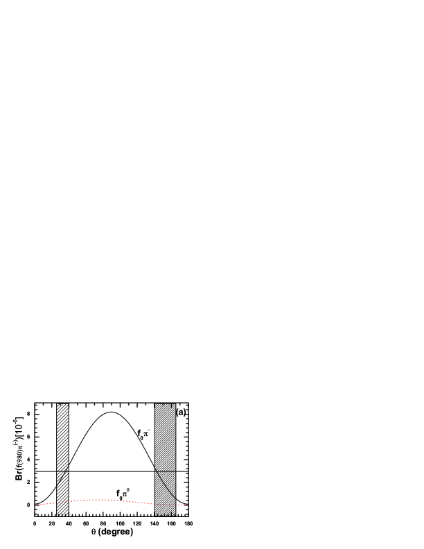
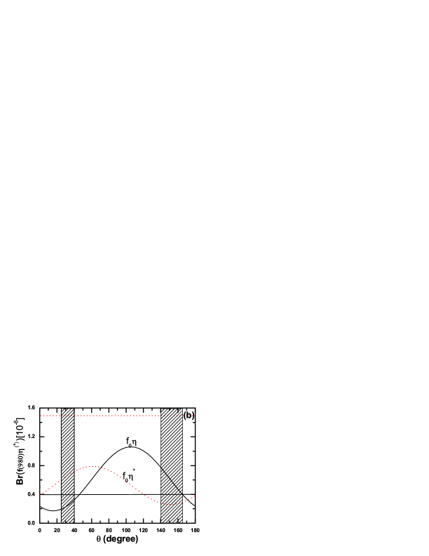
When f 0 ( 980 ) subscript 𝑓 0 980 f_{0}(980) n ¯ n ¯ 𝑛 𝑛 \bar{n}n s ¯ s ¯ 𝑠 𝑠 \bar{s}s θ 𝜃 \theta θ 1 = [ 25 ∘ , 40 ∘ ] subscript 𝜃 1 superscript 25 superscript 40 \theta_{1}=[25^{\circ},40^{\circ}] θ 2 = [ 140 ∘ , 165 ∘ ] subscript 𝜃 2 superscript 140 superscript 165 \theta_{2}=[140^{\circ},165^{\circ}] hycheng1 30 − 50 % 30 percent 50 30-50\%
Figure 2: The θ − limit-from 𝜃 \theta- B → f 0 ( 980 ) π → 𝐵 subscript 𝑓 0 980 𝜋 B\to f_{0}(980)\pi B ¯ 0 → f 0 η ( ′ ) → superscript ¯ 𝐵 0 subscript 𝑓 0 superscript 𝜂 ′ \bar{B}^{0}\to f_{0}\eta^{(\prime)}
In Fig. 2 θ − limit-from 𝜃 \theta- θ 𝜃 \theta hycheng2 hfag 2 θ 𝜃 \theta
Now we turn to the evaluations of the CP-violating asymmetries of
B → f 0 ( 980 ) π , f 0 ( 980 ) η ( ′ ) → 𝐵 subscript 𝑓 0 980 𝜋 subscript 𝑓 0 980 superscript 𝜂 ′
B\to f_{0}(980)\pi,f_{0}(980)\eta^{(\prime)} 10 − 6 ∼ 10 − 8 similar-to superscript 10 6 superscript 10 8 10^{-6}\sim 10^{-8}
Table 2: The pQCD predictions (in units of 10 − 2 superscript 10 2 10^{-2} B → f 0 ( 980 ) π , f 0 ( 980 ) η ( ′ ) → 𝐵 subscript 𝑓 0 980 𝜋 subscript 𝑓 0 980 superscript 𝜂 ′
B\to f_{0}(980)\pi,f_{0}(980)\eta^{(\prime)}
In this paper, based on the assumption of two-quark structure of the scalar meson
f 0 ( 980 ) subscript 𝑓 0 980 f_{0}(980) B → f 0 ( 980 ) π → 𝐵 subscript 𝑓 0 980 𝜋 B\to f_{0}(980)\pi B ¯ 0 → f 0 ( 980 ) η ( ′ ) → superscript ¯ 𝐵 0 subscript 𝑓 0 980 superscript 𝜂 ′ \bar{B}^{0}\to f_{0}(980)\eta^{(\prime)}