Analytical Solutions for Radiative Transfer: Implications for Giant Planet Formation by Disk Instability

Abstract

The disk instability mechanism for giant planet formation is based on the formation of clumps in a marginally-gravitationally unstable protoplanetary disk, which must lose thermal energy through a combination of convection and radiative cooling if they are to survive and contract to become giant protoplanets. While there is good observational support for forming at least some giant planets by disk instability, the mechanism has become theoretically contentious, with different three dimensional radiative hydrodynamics codes often yielding different results. Rigorous code testing is required to make further progress. Here we present two new analytical solutions for radiative transfer in spherical coordinates, suitable for testing the code employed in all of the Boss disk instability calculations. The testing shows that the Boss code radiative transfer routines do an excellent job of relaxing to and maintaining the analytical results for the radial temperature and radiative flux profiles for a spherical cloud with high or moderate optical depths, including the transition from optically thick to optically thin regions. These radial test results are independent of whether the Eddington approximation, diffusion approximation, or flux-limited diffusion approximation routines are employed. The Boss code does an equally excellent job of relaxing to and maintaining the analytical results for the vertical ($\theta$) temperature and radiative flux profiles for a disk with a height proportional to the radial distance. These tests strongly support the disk instability mechanism for forming giant planets.

1 Introduction

High precision Doppler surveys provide the best estimates to date of the frequency of gas giant planets around solar-type stars in the sun’s neighborhood of the galaxy. Cumming et al. (2008) analyzed 8 years of HIRES spectrometer data from the Keck Planet Search effort, begun in 1996, taking into account the detection threshold for each star. Cumming et al. (2008) estimated that 17% to 20% of solar-type stars have planets with masses of 0.3 $M_{J}$ (i.e., Saturn-mass) and above, orbiting within 20 AU. Considering that this estimate is based on an extrapolation to longer period orbits from detections of planets with orbital periods of 2000 days or less, this frequency estimate may well be a lower bound, if the frequency of gas giant planets continues to increase with orbital period: the frequency of gas giant planets with orbital periods less than 300 days is only 1/5 that of planets with orbital periods between 300 days and 2000 days. Gas giant planets are thought to form primarily with orbital periods greater than 2000 days, so there may well be an as yet unseen extensive population of gas giant planets with orbital periods greater than 2000 days that have not suffered inward migration. Such planets would have formed in regions with relatively short-lived outer disks (e.g., Orion, Carina), while planets formed in regions with relatively long-lived outer disks (e.g., Taurus, Ophiuchus) would have migrated inward (Boss 2005; Eisner et al. 2008).

Given this high frequency of gas giant planets, it is clear that there must be at least one efficient mechanism for gas giant planet formation. Two such mechanisms have been proposed, core accretion (e.g., Mizuno 1980) and disk instability (e.g., Boss 1997), and both appear to be necessary to explain the entire range of planets detected to date. Core accretion is the preferred mechanism for giant planets with very large inferred core masses, such as HD 149026b, which appears to have a core mass of $\sim$ 70 $M_{\oplus}$ and a gaseous envelope of $\sim$ 40 $M_{\oplus}$ (Sato et al. 2005). On the other hand, disk instability would seem to be the preferred mechanism for forming gas giants in very low metallicity systems, such as the M4 pulsar planet, where the metallicity [Fe/H] = -1.5 (Sigurdsson et al. 2003). Disk instability is also able to form gas giants around M dwarf stars (Boss 2006b), unlike core accretion (Laughlin et al. 2004; Ida & Lin 2005). Both Doppler and microlensing searches have detected gas giants in orbit around M dwarfs, most recently a 3 $M_{J}$ planet in the OGLE-2005-BLH-071L microlensing event (Dong et al. 2008). Microlensing has detected a Jupiter/Saturn analog system (Gaudi et al. 2008) around an M dwarf that is consistent with photoevaporative gas loss from an outer gas giant formed by disk instability in a region of massive star formation (Boss 2006b,c). Doppler searches have detected numerous hot super-Earths, accompanied by outer gas giant planets (e.g., HD 181433b and HD 47186b [Bouchy et al. 2008] and HD 40307bcd [Mayor et al. 2008]), a situation similar to that of our solar system and consistent with the “best of both worlds” scenario (Boss 1997), where rocky planets form by collisional accumulation inside the orbits of gas giants formed by disk instability.

In spite of this observational evidence, theoretical work on disk instability is split between those whose studies are either supportive (e.g., Boss 1997, 2000, 2001, 2005, 2006a,b,c, 2007, 2008; Mayer et al. 2002, 2004, 2007) or dismissive (e.g., Pickett et al. 2000; Cai et al. 2006, 2008; Boley et al. 2006, 2007a,b; Rafikov 2005, 2007; Stamatellos & Whitworth 2008) of disk instability being able to form giant planets. This divergence appears to be the result of a variety of modeling issues (Nelson 2006; Boss 2007), such as numerical spatial resolution, gravitational potential solver accuracy, artificial viscosity, stellar irradiation, radiative transfer, and spurious numerical heating. A combination of joint code test cases (e.g., Boss 2007) and rigorous testing is needed to try to resolve these differences.

Boley et al. (2006, 2007b) presented the results of a series of tests of their radiative hydrodynamics code on a “toy problem” (a plane-parallel grey atmosphere) with sufficient assumptions to permit an analytical solution for the vertical temperature and radiative flux profiles. This toy problem is well-suited to their cylindrical coordinate code, as their vertical cylindrical coordinate can be used to simulate a plane-parallel atmosphere. However, the Boley et al. (2006, 2007b) test cases are unsuitable for a code based on spherical coordinates (Boss 2008), as is the situation for the Boss & Myhill (1992) code used in Boss (1997, 2000, 2001, 2005, 2006a,b,c, 2007, 2008).

Boley et al. (2006) “… challenge all researchers who publish radiative hydrodynamics simulations to perform similar tests or to develop tests of their own and publish the results.” This purpose of this paper is to address this challenge by the latter route, as the former route is precluded. Two analytical solutions for radiative transfer in spherical coordinates are first derived and then used to test extensively the spherically symmetric (one dimensional, $r$) and azimuthally symmetric (two dimensional, $r$, $\theta$) versions of the Boss & Myhill (1992) three dimensional code ($r$, $\theta$, $\phi$), the same code that has been used in all of the author’s radiative hydrodynamics models of disk instability.

2 Numerical Methods

The new test calculations were performed with either the spherically symmetric or axisymmetric versions of the code that solves the three dimensional equations of hydrodynamics and radiative transfer, as well as the Poisson equation for the gravitational potential. This code has been used in all of the author’s previous studies of disk instability, and is second-order-accurate in both space and time (Boss & Myhill 1992).

For the spherically symmetric tests (R models), the equations are solved on a spherical coordinate grid with $N_{r}=101$. The radial grid ($r$) is uniformly spaced with $\Delta r=0.20$ AU between 0 and 20 AU. The gravitational potential of the spherical cloud is obtained by the tridiagonal matrix inversion technique. The boundary conditions are chosen at both 0 and 20 AU to absorb radial velocity perturbations, though we shall see that in the new test cases, the velocities are assumed to be zero, so the hydrodynamics boundary conditions are irrelevant for testing the radiative transfer routines.

For the axisymmetric tests (T models), the equations are solved on a spherical coordinate grid with $N_{r}=101$ and $N_{\theta}=22$ for $\pi/2\geq\theta>0$. Symmetry through the midplane is assumed for $\pi\geq\theta>\pi/2$. The radial grid ($r$) is uniformly spaced with $\Delta r=0.16$ AU between 4 and 20 AU, the same configuration as is typically assumed in the Boss disk instability models. The Poisson equation for the disk’s gravitational potential is solved by a spherical harmonic expansion ($Y_{lm}$) including terms up to $N_{lm}=16$. Because of the axisymmetric assumption, terms with $m\neq 0$ are dropped, reducing the solution to an expansion in Legendre polynomials. The boundary conditions are chosen at both 4 and 20 AU to absorb radial velocity perturbations, though as noted above, this is irrelevant for the radiative transfer.

3 Analytical Radiative Transfer Solutions

Boley et al. (2006, 2007b) developed test problems based on the approach taken by Hubeny (1990) in deriving simplified analytical models for the vertical structure of accretion disks. Hubeny (1990) studied one dimensional, plane-parallel atmospheres in hydrostatic equilibrium (i.e., at rest), with grey opacities and Eddington approximation radiative transfer, while neglecting convection and external radiation. Boley et al. (2007b) made similar assumptions for testing their flux-limited diffusion approximation numerical models, while also assuming constant vertical gravity, constant opacity, and constant density. We will make similar approximations here.

All of the author’s disk instability models since Boss (2001) have employed radiative transfer in the diffusion approximation, through the solution of the equation determining the evolution of the specific internal energy $E$

$${\partial(\rho E)\over\partial t}+\nabla\cdot(\rho E{\bf v})=-p\nabla\cdot{\bf v}+\nabla\cdot\bigl{[}{4\over 3\kappa\rho}\nabla(\sigma T^{4})\bigr{]},$$

where $\rho$ is the total gas and dust mass density, $t$ is time, ${\bf v}$ is the velocity of the gas and dust (considered to be a single fluid), $p$ is the gas pressure, $\kappa$ is the Rosseland mean opacity, $\sigma$ is the Stefan-Boltzmann constant, and $T$ is the gas and dust temperature. The energy equation is solved explicitly in conservation law form, as are the other hydrodynamic equations. Boss (2008) tested a flux-limiter for the diffusion approximation but found little difference between disk instability models with and without the flux-limiter.

The author’s diffusion approximation code is derived from a code that handles radiation transfer in the Eddington approximation (Boss 1984; Boss & Myhill 1992). In the Eddington approximation code, the energy equation is

$${\partial(\rho E)\over\partial t}+\nabla\cdot(\rho E{\bf v})=-p\nabla\cdot{\bf v}+L,$$

where $L$ is the rate of change of internal energy due to radiative transfer. The definition of $L$ depends on the optical depth as

$$L=4\pi\kappa\rho(J-B)\ \ \ .........\ \ \ \tau<\tau_{c},$$

$$L={4\pi\over 3}\nabla\cdot({1\over\kappa\rho}\nabla J)\ \ \ ......\ \ \ \tau>\tau_{c},$$

where $J$ is the mean intensity, $B$ is the Planck function ($B=\sigma T^{4}/\pi$), $\tau$ is the optical depth, and $\tau_{c}$ is a surface value ($\tau_{c}\sim 1$). The energy equation is solved along with the mean intensity equation for $J$, given by

$${1\over 3}{1\over\kappa\rho}\nabla\cdot({1\over\kappa\rho}\nabla J)-J=-B.$$

In the diffusion approximation, $J=B$. Hence in both the Eddington and diffusion approximations, $L$ is effectively given by

$$L={4\pi\over 3}\nabla\cdot({1\over\kappa\rho}\nabla J)$$

in optically thick regions.

In terms of the net flux vector ${\vec{H}}$, $L$ is given by

$$L=-4\pi\nabla\cdot{\vec{H}}$$

in optically thick regions (Boss 1984), and so

$${\vec{H}}=-{1\over 3\kappa\rho}\nabla J.$$

Because ${\vec{H}}={\vec{F}}/4\pi$, where ${\vec{F}}$ is the radiative flux, one also finds

$${\vec{F}}=-{4\pi\over 3\kappa\rho}\nabla J.$$

We seek a solution that decouples the radiative transfer from the hydrodynamics. As in Hubeny (1990), we assume that the test cloud or disk is at rest (${\bf v}=0$). With this assumption, the energy equation becomes

$${\partial(\rho E)\over\partial t}=L+E_{H},$$

where $E_{H}$ is a heating term constant in time. In steady state, then, the heating term must equal $-L$, so that

$$E_{H}=-{4\pi\over 3}\nabla\cdot({1\over\kappa\rho}\nabla J).$$

3.1 Radial Analytical Radiative Transfer Solutions

Assuming the spherically symmetric test cloud has constant, uniform density $\rho$ and constant, uniform opacity $\kappa$, then

$$E_{H}=-{4\sigma\over 3\kappa\rho}{1\over r^{2}}{\partial\over\partial r}\biggl{(}r^{2}{\partial T^{4}\over\partial r}\biggr{)}.$$

The following radial temperature distribution is consistent with $E_{H}$ constant in both space (inside the disk) and time

$$T(r)=T_{o}\biggl{(}2-\biggl{(}{r\over r_{o}}\biggr{)}^{2}\biggl{)}^{1/4},$$

where $T_{o}$ and $r_{o}$ are arbitrary constants. With this solution for $T(r)$, one finds that

$$E_{H}={8\sigma T_{o}^{4}\over\kappa\rho r_{o}^{2}}.$$

In optically thick regions, the radiative flux ${\vec{F}}$ is

$${\vec{F}}=-{4\sigma\over 3\kappa\rho}\nabla T^{4}.$$

Given the above temperature profile, ${\vec{F}}$ is equivalent to a scalar field $F(r)$ in the radial direction that is given by

$$F(r)={8\sigma T_{o}^{4}\over 3\kappa\rho r_{o}^{2}}r$$

in optically thick regions. The radiative flux in optically thick regions is calculated in the numerical code using

$${\vec{F}}=-{4\pi\over 3\kappa\rho}\nabla J.$$

The radius $r_{o}$ is defined to be the edge of the optically thick region, where $T(r_{o})=T_{o}$, and outside of which $T(r)=T_{o}$, i.e., the cloud is assumed to be embedded in a thermal bath at a temperature of $T_{o}=50$ K, as is commonly assumed in the Boss disk instability models. The envelope density ($r>r_{o}$) is taken to be a factor of $10^{5}$ times smaller than in the optically thick region ($r<r_{o}$), ensuring its optical thinness. The heating term $E_{H}=0$ for $r>r_{o}$, so that the radiative flux in the optically thin region must fall off with distance as $r^{2}$, i.e.,

$$F(r)={8\sigma T_{o}^{4}\over 3\kappa\rho r_{o}}\biggl{(}{r_{o}\over r}\biggr{)}^{2}$$

for $r>r_{o}$. Because the numerical code uses $L$ rather than ${\vec{F}}$ to calculate radiative transfer, there is no convenient expression for ${\vec{F}}$ in optically thin regions that can be compared to the analytical value above. In practice, the Boss disk instability models assume the presence of a thermal bath in the low optical depth regions, so the inability to compare the numerical radiative flux with the analytical value in low optical depth regions is not a problem.

3.2 Vertical Analytical Radiative Transfer Solutions

For a disk where the height is proportional to the radial distance and with constant, uniform density $\rho$ and constant, uniform opacity $\kappa$, then

$$E_{H}=-{4\sigma\over 3\kappa\rho}{1\over r^{2}sin\theta}{\partial\over\partial\theta}\biggl{(}sin\theta{\partial T^{4}\over\partial\theta}\biggr{)}.$$

The following vertical (i.e., $\theta$) temperature distribution is consistent with $E_{H}$ constant in time

$$T(\theta)=T_{o}(sin\theta)^{1/4},$$

for $\theta>\theta_{o}$, where $T_{o}$ and $\theta_{o}$ are arbitrary constants. With this solution for $T(\theta)$, one finds that $E_{H}$ varies inside the disk as

$$E_{H}=-{4\sigma T_{o}^{4}\over 3\kappa\rho}\biggl{(}{cos2\theta\over sin\theta}\biggr{)}{1\over r^{2}},$$

for $\theta>\theta_{o}$, with $E_{H}=0$ for $\theta<\theta_{o}$. Note that $E_{H}>0$ only for $3\pi/4>\theta>\pi/4$, restricting the disk thickness about the midplane to $<\pi/4$. Note that $\theta=0$ corresponds to the $\hat{z}$ axis, the rotational and symmetry axis, whereas $\theta=\pi/2$ corresponds to the equatorial plane (midplane) of the disk. The calculations all assume symmetry above and below the midplane, so that only the time evolution of the upper half of the disk is calculated.

In optically thick regions, the radiative flux ${\vec{F}}$ is equivalent to a scalar field $F(\theta)$ in the vertical direction ($\hat{\theta}$) that is given by

$$F(\theta)=-{4\sigma T_{o}^{4}\over 3\kappa\rho}{cos\theta\over r},$$

with the sign chosen to correspond to the $\theta$ coordinate, which increases downward in the disk. The radiative flux in optically thick regions is calculated in the numerical code using

$$F(\theta)=-{4\pi\over 3\kappa\rho}{1\over r}{\partial J\over\partial\theta}.$$

The angle $\theta_{o}$ is defined to be the upper edge of the optically thick disk, outside of which $T(\theta)=T_{o}(sin\theta_{o})^{1/4}$, i.e., the disk is once again assumed to be embedded in a thermal bath at a temperature of $T_{o}\approx 50$ K. The envelope density ($\theta<\theta_{o}$) is taken to be a factor of $10^{5}$ times smaller than in the optically thick region ($\theta>\theta_{o}$).

4 Results

We now present the results of two set of models that test the Boss code against these two analytical solutions. The codes used are identical to the radiative hydrodynamics codes used in the Boss disk instability models, with the exceptions being that in order to match the assumptions of the analytical solutions, the codes are restricted to either spherical symmetry or axisymmetry, the density ($\rho=10^{-10}$ g cm^-3) and opacity ($\kappa=1$ cm² g^-1) are held constant, and the velocities are all set equal to zero, so that there is no advection of energy, only heating by the $E_{H}$ term and transport by the radiative transfer term $L$. All other aspects of the Boss codes are retained, e.g., the specific internal energy and pressure subroutines and the subroutine that updates the temperature based on the specific internal energy.

4.1 Radial Test Results

Model R+50 was calculated with diffusion approximation radiative transfer. This model was started with the analytical solution for the initial temperature profile, but with a 50% temperature perturbation between 4 and 5 AU, as shown in Figure 1. Figures 1, 3, and 5 show the resulting time evolution of the numerical radial temperature profile for model R+50, while Figures 2, 4, and 6 show the corresponding evolution of the radiative flux, compared in each case to the steady state, analytical profiles (solid lines). These figures show the expected behavior in response to the initial temperature perturbation: extra radiative energy flows both inwards and outwards (Figure 2) as the cloud attempts to dispel the thermal perturbation. The perturbation extends across the entire radial extent of the cloud (Figure 3), while the radiative flux begins to return to the steady state value (Figure 4). Within a few Myr, the steady state solution is attained once again, and the code holds this solution indefinitely in time (Figures 5 and 6).

The numerical temperature profile at 14 Myr (Figure 5) is very close to the steady state value, but slightly higher in the optically thick regions inside $r_{o}=$ 10 AU. The deviations from steady state are less than 1%. Similarly, the radiative flux relaxes to very close to the analytical values, except at the center and just inside $r_{o}=$ 10 AU, where a few cells drop noticeably below the analytical solution. To the extent that these few numerical values differ from the analytical values, they err on the side of higher temperatures and lower radiative fluxes, i.e., they err on the side of discouraging cooling of the optically thick regions.

Models were also calculated with Eddington approximation radiative transfer and flux-limited diffusion approximation radiative transfer (Boss 2008), testing their ability to maintain the analytical solution. The results for these models were identical to those for models with the diffusion approximation, in the latter case because the flux-limiter was never triggered by the radiative fluxes in the optically thick regions. In all cases, the code maintains the steady state solution to the same degree that is exhibited by Model R+50 in Figures 5 and 6. Models were also calculated for a cloud with the opacity lowered by a factor of 100, i.e., $\kappa=10^{-2}$ cm² g^-1. As a result, the central optical depth dropped from $\sim 10^{4}$ in model R+50 to $\sim 10^{2}$. The lower optical depth model was calculated with the Eddington approximation code, and it maintained a temperature profile that was only slightly higher than the analytical profile throughout most of disk, again erring on the side of a slightly hotter disk.

Models were also calculated with 1% and 10% perturbations to the temperature, which behaved similarly to model R+50 except for their relaxation to the steady state value occurring faster in time, as would be expected. A model was also calculated with a negative temperature perturbation, i.e., a cloud with the temperature reduced by 50% from 4 to 5 AU. This cloud also relaxed back to the steady state solution within a few Myr, as in model R+50. Interestingly, in this model the relaxed solution was again slightly hotter than the steady state solution (by less than 1%), showing that the code relaxes to this solution independently of being approached from hotter or cooler temperatures than the steady state solution. This result implies that the radiative transfer routines, while accurate to a high degree, do result in a slight overestimate of cloud temperatures and an underestimate of the radiative fluxes, which errs on the side of discouraging disk instability’s ability to produce self-gravitating clumps.

4.2 Vertical Test Results

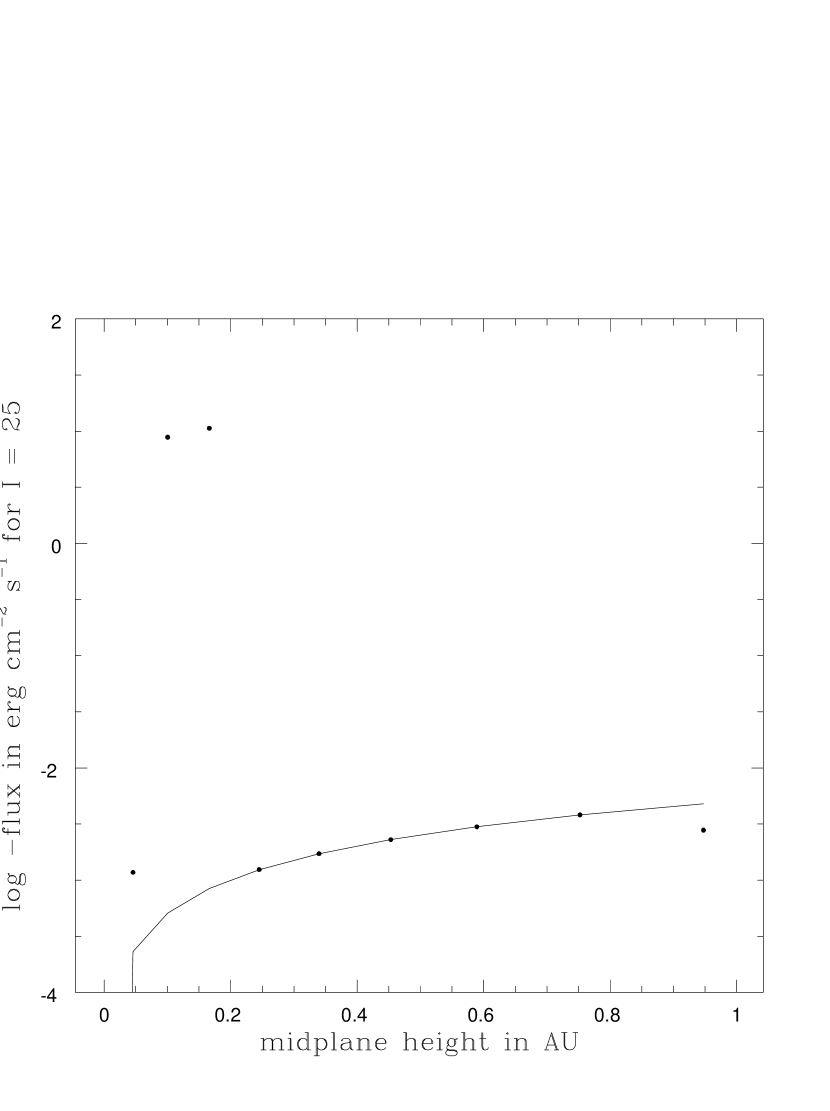
Figure 8: Same as Figure 7, but for the radiative flux profile. The radiative flux falls to zero at the midplane.

Model T+50 was also calculated with diffusion approximation radiative transfer (Eddington approximation radiative transfer becomes punitively slow in multiple dimensions, because of the need to iterate on the solution of the mean intensity equation). Model T+50 was started with the analytical solution for the initial temperature profile for a disk with $\theta_{o}=83.1$ degrees (6.9 degrees above the midplane), but with a 50% temperature perturbation between the midplane and an angle of 0.7 degrees above the midplane, as shown in Figure 7. [Note that because of the small variation with vertical height, the vertical temperature profile appears to be almost constant when plotted on the scale of the applied temperature perturbation.] Figures 7, 9, and 11 show the resulting time evolution of the numerical vertical temperature profile for model T+50, while Figures 8, 10, and 12 show the corresponding evolution of the radiative flux, compared in each case to the steady state, analytical profiles (solid lines). Once again, these figures show the expected behavior in response to the initial temperature perturbation: the upward radiative flux increases drastically in order to cool the midplane (Figure 8), raising the temperature of the entire disk (Figure 9). The radiative flux then begins to return to the steady state values (Figure 10), and by 1.9 Myr the disk has relaxed back to the analytical solution (Figure 11 and 12). The exception is a single grid point at the surface of the disk, where the flux is slightly lower than the steady state value (Figure 12), again implying an error on the side of slightly lower radiative cooling.

By way of comparison, the Boley et al. (2006) code also errs on the side of vertical disk temperatures being hotter than in the analytical solution (their Figure 17), though the differences are significantly larger than occur in the present models. The Boley et al. (2007b) code, however, does a better job of maintaining the analytical solutions.

A model like T+50 was also run starting with a 10% initial temperature perturbation. Again, the model relaxed to the analytical solutions as shown in Figures 11 and 12, only faster.

Figures 7 through 12 all depict the response of the disk at a radial distance of 7.87 AU, as that is the typical distance where clumps form in the Boss disk instability models. The behavior of the disk relaxation process at other radial distances is identical to that at 7.87 AU, except that it occurs faster at smaller radii and slower at larger radii, again as would be expected, given the larger vertical optical depths at greater radii, as the disk thickness increases proportionately.

5 Conclusions

The primary motivation for this paper was to answer the challenge issued by Boley et al. (2006) for other workers with radiative hydrodynamics codes “… to develop tests of their own and publish the results.” The new test results show that the Boss & Myhill (1992) radiative hydrodynamics code does a superb job of relaxing to and maintaining the analytical solutions for a spherical cloud or an axisymmetric disk derived here. This excellent performance is independent of whether the Eddington approximation, diffusion approximation, or flux-limited diffusion approximation is employed for the cloud, as well as of the optical depth assumed. Considering that typical disk instability calculations with the diffusion approximation last for only $\sim 10^{3}$ yr, the fact that these models show that the radiative transfer scheme is highly accurate over time scales of at least $\sim 10^{6}$ yr is reassuring for the mechanism of giant planet formation by disk instability.

These models presented here test only the radiative transfer routines and other thermodynamical aspects of the Boss codes, not the coupling between these processes and the hydrodynamics that occurs in full disk instability models. Ideally, one would test the full radiative hydrodynamics codes against analytical solutions. In the absence of such solutions, one can test the codes with respect to their ability to represent convective motions, which do involve a coupling of hydrodynamics and thermodynamics. Boss (2004) analyzed in detail the convective stability of his disk instability models, and found a good agreement between where transient, convective-like upwellings and downwellings occurred and where the Schwarzschild criterion for convection was met. Boley et al. (2007b) presented the results of several tests for convection in their codes, finding that convection occurred when it should have and did not occur when it should not have. Convection and convective-like motions thus appear to be appropriately modeled by both the Boss and Boley et al. codes.

Boss & Myhill (1992) described a variety of other tests to which the code has been subjected, including the standard nonisothermal test case for protostellar collapse (tested on two different codes by Myhill & Boss 1993), whose results have since been confirmed by Whitehouse & Bate (2006). Further tests of the Boss & Myhill (1992) code have been presented as follows: spatial resolution (Boss 2000, 2005); gravitational potential solver (Boss 2000, 2001, 2005), artificial viscosity (Boss 2006a); and radiative transfer (Boss 2001, 2007, 2008). Given the ongoing theoretical debate over the viability of disk instability for giant planet formation, it will continue to be important for other workers to conduct their own tests of these key numerical issues.

Figure 1: Analytical steady-state radial temperature profile (solid line) and numerically-calculated temperatures (solid dots) for model R+50 after 0.66 yr of evolution. The initial 50$\%$ temperature perturbation is evident between 4 and 5 AU.

Figure 2: Same as Figure 1, but for the radiative flux profile. The numerical radiative flux is less than zero (i.e., radially inward) for two grid points at 4 AU and so these two points are not shown. The radiative flux falls to zero at the center (zero radius).

Figure 3: Same as Figure 1, but after 0.071 Myr.

Figure 4: Same as Figure 3, but for the radiative flux profile. The radiative flux is less than zero (i.e., radially inward) for all the grid points interior to 3.5 AU and so these points are not shown.

Figure 5: Same as Figures 1 and 3, but after 14 Myr.

Figure 6: Same as Figure 5, but for the radiative flux profile.

Figure 7: Analytical steady-state vertical ($\theta$) temperature profile (solid line) and numerically-calculated temperatures (solid dots) for model T+50 after 0.19 yr of evolution at a radius of 7.87 AU. The initial 50$\%$ temperature perturbation is evident between the disk midplane and a height of 0.1 AU.

Figure 9: Same as Figure 7, but after 0.019 Myr.

Figure 10: Same as Figure 9, but for the radiative flux profile.

Figure 11: Same as Figures 7 and 9, but after 1.9 Myr.

Figure 12: Same as Figure 11, but for the radiative flux profile.

References

- (1)
- (2) Boley, A. C., et al. 2006, ApJ, 651, 517
- (3)
- (4) Boley, A. C., Hartquist, T. W., Durisen, R. H., & Michael, S. 2007a, ApJ, 656, L89 (erratum 660, L175)
- (5)
- (6) Boley, A. C., Durisen, R. H., Nordlund, A., & Lord, J. 2007b, ApJ, 665, 1254
- (7)
- (8) Boss, A. P. 1984, ApJ, 277, 768
- (9)
- (10) ——. 1997, Science, 276, 1836
- (11)
- (12) ——. 2000, ApJL, 536, L101
- (13)
- (14) ——. 2001, ApJ, 563, 367
- (15)
- (16) ——. 2004, ApJ, 610, 456
- (17)
- (18) ——. 2005, ApJ, 629, 535
- (19)
- (20) ——. 2006a, ApJ, 641, 1148
- (21)
- (22) ——. 2006b, ApJ, 643, 501
- (23)
- (24) ——. 2006c, ApJ, 644, L79
- (25)
- (26) ——. 2007, ApJL, 661, L73
- (27)
- (28) ——. 2008, ApJ, 677, 607
- (29)
- (30) Boss, A. P., & Myhill, E. A. 1992, ApJS, 83, 311
- (31)
- (32) Bouchy, F., et al. 2008, A&A, submitted
- (33)
- (34) Cai, K., et al. 2006, ApJL, 636, L149 (erratum 642, L173)
- (35)
- (36) ——. 2008, ApJ, 673, 1138
- (37)
- (38) Cumming, A., et al. 2008, PASP, 120, 531
- (39)
- (40) Dong, S., et al. 2008, ApJ, submitted
- (41)
- (42) Eisner, J. A., et al. 2008, ApJ, in press
- (43)
- (44) Gaudi, B. S., et al. 2008, Science, 319, 927
- (45)
- (46) Hubeny, I. 1990, ApJ, 351, 632
- (47)
- (48) Ida, S., & Lin, D. N. C. 2005, ApJ, 626, 1045
- (49)
- (50) Laughlin, G., Bodenheimer, P., & Adams, F. C. 2004, ApJ, 612, L73
- (51)
- (52) Mayer, L, Quinn, T., Wadsley, J., & Stadel, J. 2002, Science, 298, 1756
- (53)
- (54) ——. 2004, ApJ, 609, 1045
- (55)
- (56) Mayer, L, Lufkin, G., Quinn, T., & Wadsley, J. 2007, ApJL, 661, L77
- (57)
- (58) Mayor, M., et al. 2008, A&A, submitted
- (59)
- (60) Mizuno, H. 1980, Prog. Theor. Phys., 64, 544
- (61)
- (62) Myhill, E. A., & Boss, A. P. 1993, ApJS, 89, 345
- (63)
- (64) Nelson, A. F. 2006, MNRAS, 373, 1039
- (65)
- (66) Pickett, B. K., Cassen, P., Durisen, R. H., & Link, R. 2000, ApJ, 529, 1034
- (67)
- (68) Rafikov, R. R. 2005, ApJ, 621, L69
- (69)
- (70) ——. 2007, ApJ, 662, 642
- (71)
- (72) Sato, B., et al. 2005, ApJ, 633, 465
- (73)
- (74) Sigurdsson, S., et al. 2003, Science, 301, 193
- (75)
- (76) Stamatellos, D. & Whitworth, A. P. 2008, A&A, 480, 879
- (77)
- (78) Whitehouse, S. C., & Bate, M. R. 2006, MNRAS, 367, 32
- (79)