Spin-Transfer Torque in Helical Spin-Density Waves

Abstract

The current driven magnetisation dynamics of a helical spin-density wave is investigated. Expressions for calculating the spin-transfer torque of real systems from first principles density functional theory are presented. These expressions are used for calculating the spin-transfer torque for the spin spirals of Er and fcc Fe at two different lattice volumes. It is shown that the calculated torque induces a rigid rotation of the order parameter with respect to the spin spiral axis. The torque is found to depend on the wave vector of the spin spiral and the spin-polarisation of the Fermi surface states. The resulting dynamics of the spin spiral is also discussed.

I Introduction

The spin-transfer torque (STT) provides a means of manipulating the magnetisation of a material using a current. The effect was proposed from theoretical considerations by SlonczewskiSlonczewski (1996) and BergerBerger (1996) and has attracted a lot of attention due to its potential use in applications where a magnetic state is altered by a current as opposed to traditional techniques involving magnetic fields.

Most theoretical and experimental work on the STT concerns layered magnetic structures where the STT appears as a consequence of angular momentum conservation as a current traverses an interface between two regions of non-parallel magnetisation. RecentlyWessely et al. (2006) we have shown that a STT also occurs in systems with a helical spin-density wave (SDW). This was shown by a first-principles calculation of the STT for a bulk rare-earth system (Er) in its low temperature helical spin spiral (SS) structure. The effect of the current induced STT in Er is a rigid rotation of the SS order parameter. This phenomenon is a bulk effect in contrast to STT in layered systems where the STT mainly occurs close to the interfaces between the layers.

In this Article we present a more general discussion on the current induced torque in a SS. First the effect is illustrated using a one-dimensional model of a SS. We in the subsequent section present first-principles calculations of the STT for three real systems, Er and fcc Fe or $\gamma$-Fe at two different lattice volumes. Previous first-principles calculations have shown that both Er and $\gamma$-Fe have helical SDWs.Mryasov et al. (1992); Sjöstedt et al. (2000) In many other respects these two systems are very different. Erbium is one of several rare-earth elements that exhibit a helical SDW and where the ordering is driven by a nesting between parallel sheets of the Fermi surface (FS). Iron belongs to the 3d-transition metals where SDWs are less frequent. The fcc phase of Fe, which is the phase where a SS order has been found both in experiments and theory, has only been stabilised at very special conditions, and it is believed that the helical SDW is the combined result of several parts of the FS. For the one-dimensional model, as well as the considered real systems, we find that an applied current induces a STT generating a rigid rotation of the spiral order. With this theoretical prediction, new types of potential applications of the STT can be imagined, such as current driven oscillators with tunable frequencies. The current driven spin dynamics for such a device is investigated in section (VII)

II Theory

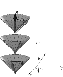
Figure 1: Local magnetisation direction of a helical spin density wave. The spin density wave is characterised by the SS wave vector ${\bf q}$, the cone angle $\theta$, and the rotation angle $\phi={\bf q}\cdot{\bf r}$.

For a system with a helical SDW, the direction of the local magnetisation rotates around the SS quantisation axis as one moves in the direction of the SS wave vector. Without loss of generality, we here consider the rotation axis to be parallel to the SS wave vector, except when explicitly stated, and will refer to it as the SS axis. Although we here consider helical SDWs, the results are valid for cycloidal SDWs as well. A SS is characterised by its SS wave vector ${\bf q}$ and its cone angle $\theta$, which is the angle between the SS axis and the local magnetisation, see Fig. 1. In this section we first consider a one-dimensional model of a SS, where the spin currents and STT are calculated analytically. We then discuss how accurate first-principles calculations of the STT can be performed.

II.1 The STT in a 1D model of a spin spiral

As a simple one-dimensional single band model of a SS system, we consider independent particles in a spin-dependent potential. The spin-dependent potential is chosen such that the ground state of the system has a helical magnetisation ${\bf M}=M{\hat{\bf m}}$ where

$${\hat{\bf m}}=(\textrm{sin}~{}\theta~{}\textrm{cos}~{}qz,~{}\textrm{sin}~{}\theta~{}\textrm{sin}~{}qz,~{}\textrm{cos}~{}\theta).$$ (1)

Here, the SS wave vector ${\bf q}=q{\hat{\bf z}}$ and $\theta$ is the cone angle. The single particle Schrödinger or Kohn Sham equation for such a model system takes the form

$$\begin{array}[]{cr}\Big{\{}-{\hbar^{2}\over 2m_{e}}{\partial^{2}\over\partial z^{2}}&+{U\over 2}\big{[}\textrm{sin}~{}\theta~{}\left(\textrm{cos}~{}qz~{}{\sigma}_{x}+\textrm{sin}~{}qz~{}{\sigma}_{y}\right)\\ &+\textrm{cos}~{}\theta~{}{\sigma}_{z}\big{]}-\epsilon\Big{\}}\psi=0,\end{array}$$

where $U$ is the exchange splitting, $m_{e}$ is the electron mass, $\hbar$ is the Planck constant $\sigma_{x},\;\sigma_{y},\;\sigma_{z}$ are the Pauli matrices and $\epsilon$ is the one particle energy. This equation can be solved analyticallyOverhauser (1962) and the eigenfunctions are the so called generalised Bloch states,

$$\psi_{k}=\left(\begin{array}[]{c}\psi_{nk}(z,\uparrow)\\ \psi_{nk}(z,\downarrow)\end{array}\right)=e^{ikz}\left(\begin{array}[]{c}\textrm{cos}~{}(\theta_{k}/2)~{}e^{-iqz/2}\\ \textrm{sin}~{}(\theta_{k}/2)~{}e^{iqz/2}\end{array}\right).$$ (2)

For the above wave function the direction of the spin ${\hat{\bf s}}$ rotates around the SS axis, with rotation angle $\phi=qz$, at an angle $\theta_{k}$ with respect to the SS axis,

$${\hat{\bf s}}(s)=(\textrm{sin}~{}\theta_{k}~{}\textrm{cos}~{}qz,~{}\textrm{sin}~{}\theta_{k}~{}\textrm{sin}~{}qz,~{}\textrm{cos}~{}\theta_{k}).$$ (3)

Note that the single electron cone angle $\theta_{k}$ and the cone angle $\theta$ of the SS, see Fig. 1, in general are different. In one dimension, the charge current $j$, induced by applying an electric field, is a scalar given by

$$j(z)=-\delta f{e\hbar\over m_{e}}Re\Big{(}\psi_{k_{F}}^{*}i{\partial\over\partial z}\psi_{k_{F}}-\psi_{-k_{F}}^{*}i{\partial\over\partial z}\psi_{-k_{F}}\Big{)},$$ (4)

where $\delta f$ is the change in occupation at the Fermi level due to the electric field, $k_{F}$ is the Fermi wave vector and $e$ is the elementary charge. In a similar way, the spin current ${\bf Q}$ due to a weak electric field is a vector given by

$${\bf Q}(z)=-\delta f{\hbar^{2}\over 2m_{e}}Re\Big{(}\psi_{k_{F}}^{*}i{\partial\over\partial z}{\mathbf{\sigma}}\psi_{k_{F}}-\psi_{-k_{F}}^{*}i{\partial\over\partial z}{\mathbf{\sigma}}\psi_{-k_{F}}\Big{)}.$$ (5)

From the spin current can the rate of change of angular momentum within an infinitesimal region of the system be calculated. The rate of change or torque on the region between $z_{0}$ and $z_{0}+dz$ is given by the spin flux into the region

$${\partial{\bf J}\over\partial t}(z_{0})=Q(z_{0})-Q(z_{0}+dz)=-{\partial{\bf Q}\over\partial z}\Big{|}_{z_{0}}dz.$$ (6)

Both the spin-flux $\partial{\bf J}/\partial t$ and the current $j$ depend on the change in occupation of the states at the Fermi level caused by the applied electric field. These two quantities are linked by the expression,

$${\partial{\bf J}\over\partial t}=\textsf{C}j,$$ (7)

which defines the torque current tensor C. The torque current tensor is in three dimensions a matrix, but becomes a vector in a one-dimensional system, where also the current vector is reduced to a scalar. For our model system, the torque current tensor can be calculated by inserting the Fermi Bloch states, $\psi_{k_{F}}$ and $\psi_{-k_{F}}$ from Eq. (2) into Eq. (4)-(5), resulting in,

$$\textsf{C}={\partial{\bf Q}\over\partial z}\Big{|}_{z_{0}}dz/j(z_{0})=a(\theta,k_{F})\left(\begin{array}[]{c}-q~{}\textrm{sin}~{}(qz_{0}){}\\ q~{}\textrm{cos}~{}(qz_{0}){}\\ 0\end{array}\right)dz,$$ (8)

where the first factor, $a(\theta,k_{F})$, depends on the spiral cone angle $\theta$ and the Fermi wave vector $k_{F}$. For planar spin spirals, where $\theta=\pi/2$, the factor reduces to a simple function of the single electron cone angle $\theta_{k}$ of the states at the Fermi level given by

$$a(\pi/2,k_{F})={\hbar\over 2e}~{}{\textrm{sin}~{}\theta_{k_{F}}\over 1-(q/2k)\textrm{cos}~{}\theta_{k_{F}}}.$$ (9)

A comparison between Eq. (1) and Eq. (8) shows that the current induced torque, in our one-dimensional model, is perpendicular to the magnetisation direction and lies in the plane of rotation of the SS, thus causing the SS to rotate with respect to the SS axis. It can also be seen from Eq. (8) that the magnitude of the STT is governed by the length of the SS wave vector $q$ and the factor $a(\theta,k_{F})$.

II.2 The STT for a real system

The STT for a real system can be calculated by generalising the expressions for the charge and spin currents in one dimension to three dimensions. In three dimensions can the currents induced by an external electric field, to linear order in the field, be calculated from a FS integral. For a multiband system must the contribution from all bands crossing the Fermi level be taken into account. In the previous section was a model system and the STT on an infinitesimal region at an arbitrary point of the system considered. For a real material, where most of the angular momentum is localised on the atoms is the time evolution of the atomic moment governed by the STT on the corresponding atom. The torque on an atom is given by the spin-flux into a sphere surrounding the atom. For a single electron state with band index $n$ and wave vector ${\bf k}$, the flux into a sphere of radius $R$ is given by,

$$-\int_{0}^{\pi}\int_{0}^{2\pi}{\bf Q}_{n{\bf k}}\cdot{\hat{\bf r}}R~{}\textrm{sin}~{}\theta~{}d\phi d\theta={\partial{\bf J}_{n{\bf k}}\over\partial t}.$$ (10)

In three dimensions is the one electron spin current tensor

$${\bf Q}_{n{\bf k}}({\bf r})=\mathrm{Re}\left\{\psi^{\dagger}_{n{\bf k}}({\bf r})\,{\bf s}\otimes{\bf v}\psi_{n{\bf k}}({\bf r})\right\},$$ (11)

where ${\bf s}=(\hbar/2){\bf\sigma}$, and ${\bf v}=(-i\hbar/m_{e})\nabla$. The total spin current is the sum of the spin currents from all occupied states. A external electric field ${\bf E}$ induces a non equilibrium spin current by changing the occupation of the states $\delta f$ at the FS. The change in occupation number $\delta f$ can be calculated using the relaxation time approximation and semiclassical Boltzmann theory,Xiao et al. (2004)

$$\delta f({\bf k})=-\delta(\epsilon_{n{\bf k}}-\epsilon_{F}){\tau e\over\hbar}\nabla_{\bf k}\epsilon_{n{\bf k}}\cdot{\bf E},$$ (12)

where $\tau$ is the electron relaxation time and $\epsilon_{n{\bf k}}$ is the band energy. The total non equilibrium torque on an atom can be calculated from a FS integral,

$${\partial{\bf J}\over\partial t}={-V_{C}\tau e\over(2\pi)^{3}\hbar}\sum_{n}\int_{FS}{\partial{\bf J}_{n{\bf k}}\over\partial t}\left(\nabla_{\bf k}\epsilon_{n{\bf k}}\cdot{\bf E}\right){dS_{n\bf k}\over|\nabla_{\bf k}\epsilon_{n{\bf k}}|}\,,$$ (13)

where $V_{C}$ is the volume of the system and a summation is performed over all bands crossing the Fermi level. The above equation defines a linear relation between the torque and the external field,

$${\partial{\bf J}\over\partial t}=\tau\sum_{n}\textsf{A}_{n}{\bf E}.$$ (14)

A similar relation can be obtained for the charge current density and the electric field,

$${\bf j} =\tau\sum_{n}\textsf{B}_{n}{\bf E}$$

$$={1\over(2\pi)^{3}}{\tau e^{2}\over\hbar^{2}}\sum_{n}\int_{FS}\nabla_{\bf k}\epsilon_{n{\bf k}}\left(\nabla_{\bf k}\epsilon_{n{\bf k}}\cdot{\bf E}\right){dS_{n\bf k}\over|\nabla_{\bf k}\epsilon_{n{\bf k}}|},$$

where $\textsf{B}_{n}$ is the conductivity tensor for band $n$. By combining Eqs. (14)-(II.2) is a linear relation between the torque and the current density obtained, where the unknown electron relaxation time $\tau$ has been cancelled,

$${\partial{\bf J}\over\partial t}=(\sum_{n}\textsf{A}_{n})(\sum_{m}\textsf{B}_{m})^{-1}{\bf j}=\textsf{C}{\bf j}.$$ (16)

The above equation defines the spin current tensor C in 3 dimensions.

II.3 The STT from the augmented plane wave (APW) method

The wave functions used in the previous section to calculate the torque current tensor C can be obtained from first principles electronic structure calculations using spin density functional theory. Several electronic structure methods use basis sets where space is divided into muffin-tin spheres surrounding the atoms and an interstitial region. This division is introduced in order to simplify the calculation of the intra and interatomic behaviour of the wave functions. When calculating the STT, a natural choice is to use the atomic augmentation (muffin-tin) sphere as the surface for evaluating the STT on the atoms. We now illustrate more in detail how the calculation may be carried out within the augmented plane wave method (APW). The APW expansion can be written as a sum of plane waves

$$\psi_{n{\bf k}}({\bf r})=\sum_{\bf G}\left(\begin{array}[]{c}a_{n{\bf k},\bf G}e^{i({\bf G}+{\bf k}-{\bf q}/2){\bf r}}\\ b_{n{\bf k},\bf G}e^{i({\bf G}+{\bf k}+{\bf q}/2){\bf r}}\end{array}\right),$$ (17)

where $\bf G$ are the reciprocal lattice vectors. The plane wave coefficients $a_{n{\bf k}}$ and $b_{n{\bf k}}$ are obtained from the first principles calculation. The spin-flux into a sphere with radius $R$ centred at an atom at site ${\bf r}_{m}$ is for plane waves given by the expression

$$\int_{0}^{\pi}\int_{0}^{2\pi}{\bf Q}_{n{\bf k}}\cdot{\hat{\bf r}}R~{}\textrm{sin}~{}\theta~{}d\phi d\theta= {\hbar R^{2}\over m_{e}}\mathrm{Re}\,\sum_{{\bf G},{\bf G^{\prime}}}-i4\pi\Big{[}$$

$$\alpha^{\dagger}{\bf s}\alpha\;a^{*}_{n{\bf k},\bf G}a_{n{\bf k},\bf G^{\prime}}e^{-i({\bf G}-{\bf G^{\prime}}){\bf r}_{m}}j_{1}(|{\bf G}-{\bf G^{\prime}}|R)\,({\bf G^{\prime}}+{\bf k}-{\bf q}/2){\cdot}({\widehat{{\bf G}-{\bf G^{\prime}}}})$$

$$+ \alpha^{\dagger}{\bf s}\beta\;a^{*}_{n{\bf k},\bf G}b_{n{\bf k},\bf G^{\prime}}e^{-i({\bf G}-{\bf G^{\prime}}-{\bf q}){\bf r}_{m}}j_{1}(|{\bf G}-{\bf G^{\prime}}-{\bf q}|R)\,({\bf G^{\prime}}+{\bf k}+{\bf q}/2){\bf\cdot}({\widehat{{\bf G}-{\bf G^{\prime}}-{\bf q}}})$$

$$+ \beta^{\dagger}{\bf s}\alpha\;b^{*}_{n{\bf k},\bf G}a_{n{\bf k},\bf G^{\prime}}e^{-i({\bf G}-{\bf G^{\prime}}+{\bf q}){\bf r}_{m}}j_{1}(|{\bf G}-{\bf G^{\prime}}+{\bf q}|R)\,({\bf G^{\prime}}+{\bf k}-{\bf q}/2){\cdot}({\widehat{{\bf G}-{\bf G^{\prime}}+{\bf q}}})$$

$$+ \beta^{\dagger}{\bf s}\beta\;b^{*}_{n{\bf k},\bf G}b_{n{\bf k},\bf G^{\prime}}e^{-i({\bf G}-{\bf G^{\prime}}){\bf r}_{m}}j_{1}(|{\bf G}-{\bf G^{\prime}}|R)\,({\bf G^{\prime}}+{\bf k}+{\bf q}/2){\cdot}({\widehat{{\bf G}-{\bf G^{\prime}}}})\Big{]},$$ (18)

where $j_{1}$ is the first spherical Bessel function and $\alpha$, $\beta$ are the up and down spinors respectively. With this expression evaluated it is straight forward to calculate the STT using Eq. (10) and Eq. (13).

III Materials with spin spiral magnetic order

Long ranged magnetic order in form of helical SDWs exists in several types of materials. Maybe the most famous is the heavy rare earth elements. They have similar valence electron structure, resulting in similar chemical structure, and all the tri-valent elements order in the hcp lattice structure with similar lattice volumes. The main difference along the series lies in the filling and magnetic moment of the localised 4$f$-electron shell. The FS of Er which is typical for the series has a strong nesting feature, i.e. two large parallel sheets of the FS. The formation of a SDW with a wave vector equal to the nesting vector allows for hybridisation removing these parts of the FS opening up a gap at the Fermi level lowering the total energy of the system. Anisotropies in the system determine whether the type of SDW preferred in the system, is a helical SDW, conical SDW or a longitudinal SDW.

Helical SDWs also exist for various 3d-transition compounds, however among the elemental 3d-transition metals the magnetic structure are less exotic at ambient conditions. It was previously shown that if certain general criteria are met, helical SDWs are formed in the transition metal series. This means that at conditions slightly different from ambient, spin spirals occur naturally indicating that this type of magnetic order is less exotic than one could believe. An example of such a system is $\gamma$-Fe the fcc phase of iron. Experimentally $\gamma$-Fe has been stabilised as precipitates in a Cu-matrix. The experimental magnetic ground state structure was found to be a SS with $\mathbf{q}=2\pi/a(0.1,0,1)$ where $a=$6.76 a.u. Several theoretical studiesMryasov et al. (1992); Sjöstedt et al. (2000); Lizarraga (2006) have mapped out the ground state magnetic structure of $\gamma$-Fe which was found to be very volume sensitive. In contrast to the rare-earth systems where the SS state is driven by nesting between two parallel sheets of the FS, the SS state of $\gamma$-Fe is not promoted by a single FS nesting vector. Instead there is a net energy gain from many parts of the FS given by the hybridisation by a SS vector.

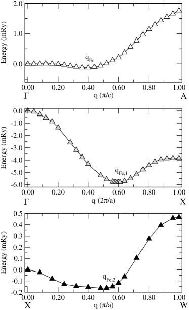
Figure 2: The top panel shows the total energy of Er per hcp unit cell for SS wave vectors from $\Gamma$ to $A$. The middle panel shows the total energy per atom of $\gamma$-Fe for SS vectors from $\Gamma$ to $X$ in the larger lattice volume. The bottom panel shows the total energy per atom of $\gamma$-Fe for SS vectors from $X$ to $W$ in the smaller lattice volume.

IV Electronic structure calculation

All the materials specific parameters for Er and $\gamma$-Fe used for the calculation of the torque current tensor C were obtained from first principles density functional theory. The calculations were made using the full-potential augmented plane wave plus local orbitals (APW+lo) method as described in Ref. Sjöstedt and Nordström, 2002. For Er, the calculations were performed in the same manner as in Ref. Nordström and Mavromaras, 2000; Wessely et al., 2006 and for $\gamma$-Fe the calculations were performed in the same way as in Ref. Sjöstedt et al., 2000; Lizarraga, 2006. The local spin density approximation (LSDA) as parametrised by von Barth and Hedin was used without any shape-approximation to the non-collinear magnetisation, i.e. charge and magnetisation densities as well as their conjugates potentials are allowed to vary freely in space both regarding magnitude and direction. For Er, a set of 12$\times$12$\times$8 k-points was used for converging the electron density and for Fe we used a set of 20$\times$20$\times$20 k-points. The SS was treated using the generalised Bloch theorem. The Er calculation was performed with the 4$f$-electrons treated as spin polarised core electrons and we used the experimental Er hcp lattice parameters ($a=6.73$ a.u. and $c=10.56$ a.u.). For Er, we calculate a large number of SS wave vectors, $\mathbf{q}=\pi/c(0,0,q)$ in the first Brillouin zone of the hcp lattice, along the out of plane direction between $\Gamma$ and $A$. The total energy for these calculations are presented in Fig. 2. There is an energy minimum for $q=0.40$ which corresponds to the ground state SS structure of Er. For Fe we perform calculations at two lattice volumes. At a lattice constant of $a=6.82$ a.u., corresponding to the lattice constant of Cu, we do a series of calculations for ${\bf q}_{1}=2\pi/a(0,0,q)$, between $\Gamma$ and $W$ in the first Brillouin zone, and an energy minimum is found for $q=0.59$ (see middle panel in Fig. 2). At a reduced lattice constant of $a=6.66$ a.u. we do a series of calculations for ${\bf q}_{2}=\pi/a(w,0,2)$, between $W$ and $X$, where there is a weak local energy minimum at $w=0.48$. This latter minimum corresponds to a spiral wave vector which is close to the experimental SS of $\gamma$-Fe. Note that ${\bf q}_{2}$ is non-parallel to the SS rotation axis which is in the ${\hat{\bf z}}$-direction for all three calculations.

V Results

In this section we present the results of the STT calculations for the three SS systems treated in the previous section. The one electron spin current tensor ${\bf Q}_{n{\bf k}}$ was calculated using Eq. (18) and the Kohn-Sham eigenfunctions obtained from the first principles calculation. The first Brillouin zone was covered by a $41\times 41\times 41$ k-point mesh, in order to accurately evaluate the FS integrals in Eq. (13) and Eq. (II.2). The conductance tensor, $\textsf{B}=\sum_{m}\textsf{B}_{m}$, was as expected, found to be diagonal for all three considered systems.

The torque current tensor C was calculated for Er having a SS with wave vector ${\bf q}=\pi/c(0\;0\;0.4)$. We found that for an Er atom situated at a site with magnetisation direction $(1\,0\,0\,)$, the spin current tensor

$$\textsf{C}={\hbar\over e}\left(\begin{array}[]{ccc}0.0&0.0&0.0\\ 0.0&0.0&-0.5\\ 0.0&0.0&0.0\\ \end{array}\right)[\textrm{\AA}^{2}].$$

From the structure of the C tensor, it can be seen that for a current in the $(0\,0\,1\,)$ direction, a torque is induced in the $(0\,1\,0\,)$ direction. Since the torque is perpendicular to the local magnetisation and lies in the SS rotation plane, we conclude that a current along the SS axis causes a rigid rotation of the SS around the SS axis.

a: Er
$n$	$(\hbar/e)(\textsf{A}_{n})_{23}$ [ÅeV]	$(\hbar^{2}/e^{2})(\textsf{B}_{n})_{33}$ [eV/Å]
1	0.01	0.006
2	0.01	0.01
3	-0.04	0.03
4	-0.008	0.007

b: Fe q1
$n$	$(\hbar/e)(\textsf{A}_{n})_{23}$ [ÅeV]	$(\hbar^{2}/e^{2})(\textsf{B}_{n})_{33}$ [eV/Å]
1	-0.002	0.002
2	0.01	0.02
3	-0.1	0.07
4	-0.005	0.002

c: Fe q2
$n$	$(\hbar/e)(\textsf{A}_{n})_{21}$ [ÅeV]	$(\hbar^{2}/e^{2})(\textsf{B}_{n})_{11}$ [eV/Å]
1	0.005	0.006
2	0.02	0.01
3	0.02	0.02
4	-0.05	0.05
5	0.09	0.08

Table 1: The elements of the $\textsf{A}_{n}$ and $\textsf{B}_{n}$ tensors that mainly contribute to the C tensor, see Eq. (16)

For $\gamma$-Fe with the larger volume in the ${\bf q}_{1}=2\pi/a(0,0,0.59)$ spiral state, the torque current tensor, evaluated for an atom with magnetisation direction $(1\,0\,0\,)$,

$$\textsf{C}={\hbar\over e}\left(\begin{array}[]{ccc}0.0&0.0&0.0\\ 0.0&0.0&-1.4\\ 0.0&0.0&0.0\\ \end{array}\right)[\textrm{\AA}^{2}].$$

Also in this case we conclude that a current along the SS axis causes a rigid rotation of the SS. In this system, the torque, for the same current density, is found to be nearly three times larger than for Er. We will return to a discussion on the magnitude of the torque later in this section.

Finally we calculated the STT in $\gamma$-Fe with reduced volume, where the SS wave vector ${\bf q}_{2}=\pi/a(0.48,0,2)$ is non parallel to the spin rotation axis ${\hat{\bf z}}$. We found that the torque current tensor for an atom with magnetisation in the $(1\,0\,0\,)$ direction is given by,

$$\textsf{C}={\hbar\over e}\left(\begin{array}[]{ccc}0.0&0.0&0.0\\ 0.6&0.0&0.0\\ 0.0&0.0&0.0\\ \end{array}\right)[\textrm{\AA}^{2}].$$

The structure of the torque current tensor for this system differs from the previous two systems. Here, a current in the $(1\,0\,0\,)$ direction is required to produce a rotation of the SS. The STT from a current in the $(0\,0\,1\,)$ direction vanish since $\gamma$-Fe with ${\bf q}_{2}=\pi/a(0.48,0,2)$ is antiferromagnetic in the $(0\,0\,1\,)$ direction.

VI Discussion

In general, the STT depends on a balance between the size of the SS wave vector and the spin polarisation of the conduction electrons at the FS.

Some insight into the origin of the STT on the single electron level can be obtained by considering the semi-classical expression for the spin current Xiao et al. (2006)

$${\bf Q}(z)={\hbar\over 2}{\hat{\bf s}}(z){j\over e}.$$ (19)

If the semi-classcal spin current is combined with Eq. (8) one obtains the following expression for the torque current tensor.

$$\textsf{C}={\hbar\over 2e}{\partial{\hat{\bf s}}(z)\over\partial z}\Big{|}_{z_{0}}dz={\hbar\over 2e}~{}\textrm{sin}~{}\theta_{k_{F}}\left(\begin{array}[]{c}-q~{}\textrm{sin}~{}(qz_{0}){}\\ q~{}\textrm{cos}~{}(qz_{0}){}\\ 0\end{array}\right)dz,$$ (20)

The above equation gives the same result as the quantum mechanical calculation of C in section  (II.1), if the denominator of the factor $a$ in Eq. (9) is equal to one, which is approximately true if $(q/2k)\textrm{cos}~{}\theta_{k_{F}}$ is small. Semi-classically, the maximum spin transferred per electron, for a given value of $q$, to an atomic layer is given by $(\hbar/2)ql$ where $l$ is the inter layer distance. This maximum can be achieved if the single electron cone angle $\theta_{k_{F}}$ is equal to $\pi/2$. For Er and $\gamma$-Fe with the larger volume is the semi-classical maximum of the spin-transfer, with the given value of $q$, equal to $0.3\hbar$ and $0.9\hbar$, respectively. A more accurate value for the average spin transferred per electron to an atom is obtained by multiplying the torque current tensor with $e/A$ where $A$ is the area per atom in the direction of the current. For Er, where the area per atom in the $(0\,0\,1\,)$ direction $A=a^{2}{\sqrt{3}}/2$, the spin-transferred per electron is $0.05\hbar$. For $\gamma$-Fe, the area per atom in the $(0\,0\,1\,)$ direction is $a^{2}/2$ and the spin-transferred per electron is $0.2\hbar$, for the larger volume. Hence, the spin-transfer torques for Er and $\gamma$-Fe (larger volume) obtained from the first principles calculations are only 16% and 22%, respectively, of the their semi-classical maximum. This is partially due to the fact that the cone angle $\theta_{k_{F}}$ of the conduction electrons is less than $\pi/2$.

Another reason for the reduced STT is that contributions from different bands partly cancel each other. The contributions from the individual bands to the STT are given by the $\textsf{A}_{n}$ and $\textsf{B}_{n}$ tensors shown in Table (1). For Er there are four bands that cross the FS and the dominant element in the $\textsf{A}_{n}$ tensors is their $(\textsf{A}_{n})_{23}$ elements. As shown in Table (1a), the STT from band three is four times larger and in the opposite direction to the STT from band one and two. For $\gamma$-Fe (larger volume) there are four bands crossing the Fermi level, where the dominating contribution to the STT comes from the third band, see Table (1b). For $\gamma$-Fe with the smaller volume there are five bands crossing the Fermi level and the dominant element in the $\textsf{A}_{n}$ tensors is their $(\textsf{A}_{n})_{21}$ elements. As shown in table (1c), the largest contribution to the STT is here coming from the fifth FS. Finally we would like to note that semi-classically the maximal spintransfer per conduction electron is $\hbar/2$, which only can be obtained if both $ql=\pi/2$ and $\theta_{k_{F}}=\pi/2$. An other route to high spin transfer is to try to reduce the denominator in the expression for the $a$ factor in Eq. (9). The $a$ factor becomes large for small Fermi surfaces where $q/k$ is large.

VII Dynamics

We will for our SS systems represent the uniform magnetisation of an atomic plane perpendicular to the SS axis by a unit vector ${\hat{\bf m}}$ in the direction of the magnetisation. The time evolution of ${\hat{\bf m}}$ is phenomenologically described by the LLG equation Landau et al. (1980); Gilbert (1955).

$${d{\hat{\bf m}}\over dt}={\bf\Gamma}-\alpha{\hat{\bf m}}\times{d{\hat{\bf m}}\over dt}.$$ (21)

The first term ${\bf\Gamma}$ is the total torque exerted on the layer and the second term is the Gilbert damping term with damping constant $\alpha$. The systems under consideration are all having a helical SDW with an easy-plane or hard-axis anisotropy. The hard-axis is directed along the SS axis and helps maintain the planar structure of the SS. For such systems is the total torque ${\bf\Gamma}$ a sum of a current induced STT and a torque resulting from the hard-axis anisotropy. Both of these torques are perpendicular to the magnetisation ${\hat{\bf m}}$ and the SS axis which here is considered to be in the ${\hat{\bf z}}$ direction. Eq. (21) can therefore for this system be written as

$${d{\hat{\bf m}}\over dt}=A{\hat{\bf m}}\times{\hat{\bf z}}-\alpha{\hat{\bf m}}\times{d{\hat{\bf m}}\over dt},$$ (22)

where

$$A(j,\theta)={q~{}j~{}a(\theta,k_{F})\over\textrm{sin}~{}\theta~{}}+b\>{\bf m}\cdot{\bf z}.$$ (23)

The first term in the above equation is due to the STT and the factor $a(\theta,k_{F})$ was introduced in Eq. (8). The $b$ in the second term is the strength of the hard-axis anisotropy. Eq. (22) is in spherical coordinates, see Fig. 1, given by.

$${d\phi\over dt}(1+\alpha^{2})=-A(j,\theta)$$ (24)

and

$${d\theta\over dt}(1+\alpha^{2})=-\alpha A(j,\theta)~{}\textrm{sin}~{}\theta.$$ (25)

Eq. (24) describes a rigid rotation of the SS due to the current induced torque where the angular velocity, as a function of the current $j$, is given by $-A(j,\theta)/(1+\alpha^{2})$. It can be seen from Eq. (25) that the effect of the Gilbert damping is to change the cone angle of the SS. Eventually, the spiral will reach a steady state with a cone angle $\theta_{0}$, given by

$${q~{}j~{}a(\theta_{0},k_{F})\over\textrm{sin}~{}\theta_{0}~{}}=-b~{}\textrm{cos}~{}\theta_{0}~{},$$ (26)

when the current induced torque and the anisotropy torque balance each other. At this point in time, also the rotational motion of the magnetic moments with respect to the SS axis stops. The polar angle $\phi$ will thus, when a current $j$ is passed along the SS axis, change by

$$\Delta\phi=-{1\over 1+\alpha^{2}}\int_{\pi\over 2}^{\theta_{0}}A(j,\theta)\Big{(}{d\theta\over dt}\Big{)}^{-1}d\theta$$ (27)

or

$$\Delta\phi={1\over\alpha}\left[\textrm{ln}\left(\textrm{tan}~{}{\pi\over 4}~{}\right)-\textrm{ln}\left(\textrm{tan}~{}{\theta_{0}\over 2}~{}\right)\right],$$ (28)

before the spiral reach the steady state with cone angle $\theta_{0}$. The SS will returns to a planar state if the current is switched off after the steady state is reached. During the reversal, the spiral rotates in the opposite direction performing the same number of rotations as required to reach the steady state.

The current induced torque has, for slowly varying magnetisation, been described by introducing an adiabatic and a non-adiabatic term in the LLG equation Li and Zhang (2004); Zhang and Li (2004); Kohno et al. (2006); Edwards and Wessely (2008). The adiabatic term, which for a SS whose axis is along ${\hat{\bf z}}$ takes the form $\partial{\hat{\bf m}}/\partial z$, has in Eq. (22) been replased by the STT component of $A(j,\theta)$. A non-adiabatic torque term proportional to ${\hat{\bf m}}\times(\partial{\hat{\bf m}}/\partial z)$ could also be introduced in Eq. (22). The main effect of such a torque would be a modification of Eq. (25), which determines the dynamics of the cone angle $\theta$. A non-adiabatic torque would add a term to the right hand side of Eq. (25) which could decrease or even change the sign of $d\theta/dt$.

The effect of in plane anisotropy is discussed in Ref. Wessely et al., 2006, where it is suggested that the current needs to overcome a certain critical current before the spiral start to rotate.

VIII Summary and conclusions

We have shown in general, that the a current through a SS induces a rotation of the spins, where the angular velocity depends on the magnitude of the current. The size of the STT has been analysed in terms of the spin-transfer per conduction electron and we conclude that the total STT depends on, the spin-polarisation of the electrons, the SS wave vector and how contributions from different bands coincide. The dynamics of the SS has been calculated including the effects of anisotropies and damping. For a system with a hard-axis anisotropy along the SS axis, the damping leads to a steady state where the rotation eventually stops.