Impurity Potential Renormalization by Strong Electron Correlation

Abstract

Renormalization of non-magnetic impurity potential by strong electron correlation is investigated in detail. We adopt the $t$-$t^{\prime}$-$t^{\prime\prime}$-$J$ model and consider mainly a $\delta$-function impurity potential. The variational Monte Carlo method shows that impurity potential scattering matrix elements between Gutzwiller-projected quasi-particle excited states are as strongly renormalized as the hopping terms. Such renormalization is also seen by the Bogoliubov-de Gennes equation with an impurity, where the strong correlation is treated by a Gutzwiller mean-field theory with local renormalization factors and local chemical potentials. Namely, the $\delta$-function potential is effectively weakened and broadened. We emphasize the importance of including the local chemical potential, which is paid little attention to in the literature, by physical consideration of the doping dependence of a local hole density. We also investigate effect of smooth impurity potential variation; the strong correlation yields anticorrelation between the gap energy and the coherence peak height simultaneously with large gap distribution, which is consistent with the experiments.

I Introduction

Anderson’s theorem tells us that the $s$-wave superconductivity is insensitive to small potential scattering Anderson59 . On the other hand, the $d$-wave superconductivity has zero superconducting gap in the nodal direction, and thus may be sensitive to disorder. However, experimental observation of the high-temperature superconductivity, which many people are nowadays convinced has $d$-wave symmetry, seems robust against disorder McElroyPRL05 ; PasupathySci08 ; ZhouPRL04 ; ShenSci05 . For example, the high-temperature superconductors seem to exhibit more conventional behavior at higher hole doping rates where the systems are supposed to be more disordered. Furthermore, the local density of states measured by the STM Fang06 ; Kohsaka07 show clear V-shape at low energy that indicates the $d$-wave nodes are not much influenced by disorder. Theoretically, it is proposed that this protection of V-shape is due to strong Coulomb repulsion between electrons Anderson00 ; Garg08 ; FukushimaSNS . Hence, detailed studies of effects of strong correlation for impurity scattering are necessary.

In correlated systems, the model parameters are effectively renormalized. For example, a hopping term is renormalized by a factor smaller than unity because hopping is more difficult in the presence of the double occupancy prohibition. On the other hand, an exchange term is renormalized by a factor larger than unity because each site is more often singly occupied. Then, the question is: how are impurity terms renormalized? In our previous paperFukushimaSNS , we have presented preliminary results of the impurity renormalization. That is, local modulations of the hopping and the exchange term tend to be enhanced by the local renormalization factors, and impurity potential tends to be screened by the effective local chemical potentials originated from minimization of the total energy. In this paper, we investigate in more detail how impurity potential is renormalized, using the variational Monte Carlo (VMC) method and the Gutzwiller-projected Bogoliubov-de Gennes (BdG) equationQHWang06 ; CLi06 ; Fukushima08 , then discuss agreement and disagreement with the experiments.

An extensive amount of literature has been devoted for the impact of impurities on the normal and superconducting state of the cuprates. A detailed review dedicated to this subject was recently given by Alloul et al. Alloul09 We do not repeat the whole review here, but the theoretical side may be summarized as follows: Suppose electrons in host metal interact with each other by the onsite repulsive Hubbard $U$ terms, and let us put a non-magnetic impurity in it. Then, very strong impurity potential (unitary scatterer), such as a cavity in otherwise uniform systems, tends to induce local magnetic moments near the impurity if $U$ is large enough, whereas weak potential (Born scatterer) does not.

However, the local moment formation in the superconducting state seems relatively controversial. The moments appear according to the theory based on the mean-field decoupling of the $U$ term, e.g., by Chen and Ting YChen2004 , and Harter et al. Harter2007 . Although it can be a good approximation for small $U$, yet antiferromagnetic correlation is probably underestimated especially at large $U$ because the superexchange process is not taken into account explicitly. Considering that the local moments typically appear at sufficiently large $U$, it is critical to know in what range of $U$ the theory is valid. An interesting contrast is in the theory by Tsuchiura et al. Tsuchiura01 based on the one-site removed $t$-$t^{\prime}$-$J$ model, i.e., an effective $U\rightarrow\infty$ model. They adopted two different Gutzwiller approximations that lead to two different BdG equations. One of them takes away the double occupancy prohibition in return for the uniform renormalization of model parameters. This calculation results in the local moment formation. It also indicates that $J$ may cause the appearance of the local moment even if $U=0$ because this effective model is a “$U=0$ but finite $J$” system. In the other BdG equation of them, each local model parameter is dressed with an extended Gutzwiller renormalization factor that depends on the position. This calculation in contrast results in the absence of the local moments because electrons tend to avoid the impurity and the antiferromagnetism locally collapses. However, these local renormalization factors are, without local derivation, speculated from the previously derived formula for the uniform system Ogata03 , and may need to be verified in the future studies. Tsuchiura’s work was criticized by Wang and Lee ZWang02 , who applied an inhomogeneous slave-boson mean-field theory to essentially the same model. The result shows the local magnetic moments in the underdoped region. In the slave-boson mean-field theory, the double occupancy prohibition is relaxed by the saddle point approximation and only its average is satisfied, which probably reduces the influence of the spin-spin interaction effectively. To compensate it, Wang and Lee added a phenomenological residual spin-spin interaction term, and the result depends on its magnitude. In addition, Gabay et al. Gabay08 recently obtained similar results. Liang and LeeLiang02 applied the VMC and also concluded that local moments appear in the underdoped regime.

The strong scatterers introduced above are modeled on in-plane impurities which substitute for Cu in the CuO₂ planes. Besides such unitary scatterers, all cuprate materials are doped by out-of-plane ions that mostly occupy random positions in the crystal lattice or interstitial positions. Such intrinsic impurities may be weak, but can be poorly screened by electrons around them because the cuprates are quasi–two-dimensional metal. In addition, these weak potentials are not expected to induce local magnetism. Influence of these “Born scattering potentials” on the local density of states was studied by, e.g., Wang and Lee, QHWangDHLee03 , and Nunner et al. Nunner05 In fact, however, the effect of electron correlation on them seems hardly discussed in the literature, with the exception of Garg et al. Garg08 , Fukushima et al. FukushimaSNS , and Andersen and Hirschfeld Andersen08 . That is a subject we would like to address in this paper.

After we define our model in Sec. II, the renormalization of impurity-potential matrix elements is shown by the VMC calculation in Sec. III. Then, the BdG equation based on the Gutzwiller approximation with local renormalization factors QHWang06 ; CLi06 ; Fukushima08 are solved in Sec. IV, where we emphasize the importance of including local chemical potentials through the comparison with the method by Garg et al. Garg08 Note that these local chemical potentials are introduced for minimizing the total energy and are different from those used for the inhomogeneous slave-boson mean-field theoryZWang02 ; Gabay08 ; Ziegler98 that are the Lagrange multipliers to enforce the average no-double-occupancy condition. Renormalization of smoothly varying impurity potential is also presented to show anticorrelation between the gap energy and the coherence peak height compatible with large gap distribution, which is consistent with the experiments Fang06 ; McElroySci05 .

II Model

We use the $t$-$t^{\prime}$-$t^{\prime\prime}$-$J$ model with an impurity term, namely,

$$H\equiv H_{tt^{\prime}t^{\prime\prime}}+H_{J}+H_{\rm imp},$$ (1)

$$H_{tt^{\prime}t^{\prime\prime}}\equiv P\left(-\sum_{i,j,\sigma}t_{ij}c_{i\sigma}^{\dagger}c_{j\sigma}\right)P$$ (2)

$$H_{J}\equiv J\sum_{\langle i,j\rangle}\left({\bf S}_{i}\cdot{\bf S}_{j}-\frac{1}{4}\hat{n}_{i}\hat{n}_{j}\right),$$ (3)

where $c_{i\sigma}^{\dagger}$ ($c_{i\sigma}$) is the creation (annihilation) operator of site $i$ and spin $\sigma$, and $\hat{n}_{i}\equiv\sum_{\sigma}c_{i\sigma}^{\dagger}c_{i\sigma}$. As the hopping, we take $t_{ij}=t,t^{\prime},t^{\prime\prime},$ for the nearest, second, and third neighbors, respectively, and otherwise zero. The summation in the $J$ term is taken over every nearest-neighbor pair. The Gutzwiller projection operator $P$ prohibits electron double occupancy at every site.

In this paper, we focus on the renormalization of a single non-magnetic $\delta$-function impurity potential located at $i=0$,

$$H_{\rm imp}=V_{0}\sum_{\sigma}c_{0\sigma}^{\dagger}c_{0\sigma}=\frac{V_{0}}{N_{L}}\sum_{k,k^{\prime}\sigma}c_{k\sigma}^{\dagger}c_{k^{\prime}\sigma},$$ (4)

except for Sec. IV.4, where we briefly discuss the effect of smoothly varying impurity potential. Here, $N_{L}$ is the number of sites.

III Variational Monte Carlo calculation for matrix element renormalization

Here we calculate matrix elements of the impurity potential with respect to the uniform Gutzwiller-projected quasi-particle states of $d$-wave superconductors using the VMC method.

Let us start from a uniform system without impurities. We assume that the ground state is well approximated by a Gutzwiller-projected $d$-wave superconducting state,

$$|{\rm GS}\rangle\propto P\left[\sum_{p}\frac{v_{p}}{u_{p}}\,c_{p\uparrow}^{\dagger}c_{-p\downarrow}^{\dagger}\right]^{\frac{N_{e}}{2}}|0\rangle,$$ (5)

where

$$u_{k}\equiv\sqrt{\frac{1}{2}\left(1+\frac{\xi_{k}}{E_{k}}\right)},\quad v_{k}\equiv\frac{\Delta_{k}}{|\Delta_{k}|}\sqrt{\frac{1}{2}\left(1-\frac{\xi_{k}}{E_{k}}\right)},$$

$$E_{k}\equiv\sqrt{\xi_{k}^{2}+\Delta_{k}^{2}},\quad\Delta_{k}\equiv\Delta_{\rm v}\,(\cos k_{x}-\cos k_{y}),$$

$$\xi_{k}\equiv-2t_{\rm v}(\cos k_{x}+\cos k_{y})-4t_{\rm v}^{\prime}\cos k_{x}\cos k_{y}$$

$$-2t_{\rm v}^{\prime\prime}(\cos 2k_{x}+\cos 2k_{y})-\mu_{\rm v}.$$

$N_{e}$ is the total number of electrons. The variational parameters $\Delta_{\rm v}$, $t_{\rm v}^{\prime}$, $t_{\rm v}^{\prime\prime}$, $\mu_{\rm v}$ are optimized so as to minimize the total energy. We also assume that the excited states are well represented by the projected quasi-hole wave functionCPChouJMMM07 ,

$$|k\sigma\rangle\propto P\,c_{k\sigma}^{\dagger}\left[\sum_{p}\frac{v_{p}}{u_{p}}c_{p\uparrow}^{\dagger}c_{-p\downarrow}^{\dagger}\right]^{\frac{N_{e}}{2}-1}|0\rangle.$$ (6)

Then, we are able to calculate the matrix elements and spectral weights using the excited quasi-hole wave function with the ground state parameters.

By switching on the impurity potential, these excited states should be mixed by the matrix elements,

$$V_{k,k^{\prime}}\equiv\langle k\uparrow|c^{\dagger}_{k\uparrow}c_{k^{\prime}\uparrow}|k^{\prime}\uparrow\rangle+\langle-k^{\prime}\uparrow|c^{\dagger}_{k\downarrow}c_{k^{\prime}\downarrow}|-k\uparrow\rangle.$$ (7)

We carry out VMC calculation for $V_{k,k^{\prime}}$, and show that its renormalization by the strong correlation is similar to that of the total spectral weight,

$$Z_{k}\equiv\Big{|}\langle{k\sigma}|c_{k\sigma}^{\dagger}|{\rm GS}\rangle\Big{|}^{2}+\Big{|}\langle{k\sigma}|c_{-k-\sigma}|{\rm GS}\rangle\Big{|}^{2},$$ (8)

which is known to be strongly renormalized CPChou06 . It is worthy to be noted that the BCS theory has predicted the matrix elements of the impurity potential and the total spectral weights are $V_{k,k^{\prime}}^{\rm BCS}=u_{k}u_{k^{\prime}}-v_{k}v_{k^{\prime}}$, and $Z_{k}^{\rm BCS}=1$, respectively. On the other hand, the Gutzwiller approximation (GA) yields renormalization,

$$Z_{k}^{\rm GA}=g_{t}\equiv\frac{2x}{1+x},$$ (9)

where $g_{t}$ is the Gutzwiller renormalization factor for the hopping term. However, according to the conventional GA, $V_{k,k^{\prime}}$ is not renormalized because it originally comes from a particle number operator; on the contrary, a GA generalized for inhomogeneous systems yields renormalization as will be discussed in the next section.

We plot $V_{k,k^{\prime}}/V_{k,k^{\prime}}^{\rm BCS}$ and $Z_{k}/Z_{k}^{\rm BCS}$ in Fig. 1 as functions of the hole concentration. Suppose the impurity potential is not too large. Then, the matrix elements $V_{k,k^{\prime}}$ perturb the system only if the excitation energies of $|{k\sigma}\rangle$ and $|{k^{\prime}\sigma}\rangle$ are close. Therefore, here we plot $V_{k,k^{\prime}}$ connecting two symmetric reciprocal lattice points indicated in the inset of Fig. 1; each pair of symbols in the inset refers to $k$ and $k^{\prime}$, which corresponds to the same symbols of $V_{k,k^{\prime}}$ and $Z_{k}=Z_{k^{\prime}}$ in the plot. The variational parameters are optimized for each hole concentration. Note that $V_{k,k^{\prime}}$ is renormalized as strongly as $Z_{k}$, and its renormalization factor is quite close to $g_{t}$. Furthermore, Fig. 2 compares $V_{k,k^{\prime}}$ of different bare parameters in the Hamiltonian. It suggests that the renormalization is insensitive to parameters.

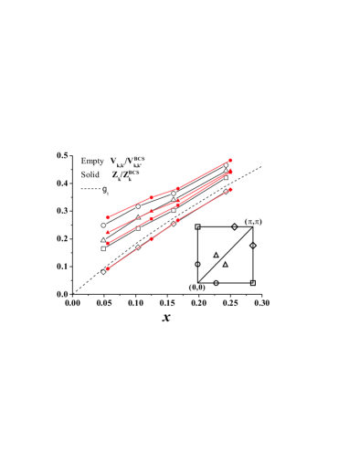
Figure 1: (Color online) Comparison of $V_{k,k^{\prime}}/V_{k,k^{\prime}}^{\rm BCS}$ and $Z_{k}/Z_{k}^{\rm BCS}$ as functions of the hole concentration $x$ in the case of $(t^{\prime},t^{\prime\prime},J)/t=(-0.3,0.2,0.3)$ optimized at each $x$. Each symbol represents transfer between the $k$-points of the same symbols in the inset.

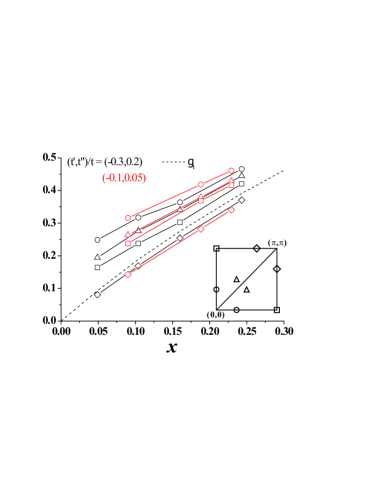
Figure 2: (Color online) Comparison of $V_{k,k^{\prime}}/V_{k,k^{\prime}}^{\rm BCS}$ of different bare parameters. Each symbol represents transfer between the $k$-points of the same symbols in the inset.

These results may be understood as follows. Let us look at the Fourier transform of the $\delta$-function impurity potential [Eq. (7)]. The sum of its diagonal terms $(k=k^{\prime})$ just slightly shifts the chemical potential. What about the off-diagonal terms $(k\neq k^{\prime})$? If $k$ were a site index, they would be renormalized as $g_{t}=2x/(1+x)$ according to the Gutzwiller approximation, which is smaller than unity and is going to zero as $x\rightarrow 0$ because it is more difficult to hop in the presence of the double occupancy prohibition. Even in $k$ space, if electrons are densely packed in the lattice, it must be similarly difficult to hop from $k$ to a different $k^{\prime}$. Thus, the impurity potential should be renormalized by a factor similar to $g_{t}$ as we expected.

IV Gutzwiller-projected Bogoliubov-de Gennes equation

IV.1 Renormalization by effective local chemical potentials

We solve a BdG equation derived using the Gutzwiller approximation with local renormalization factorsQHWang06 ; CLi06 ; Fukushima08 for non-magnetic systems. By requiring minimization of the total energy, the BdG Hamiltonian naturally contains effective local chemical potentials originating from the derivative of the local renormalization factors with respect to local particle densities. In the following, we show that the impurity potential is renormalized by those local chemical potentials.

Let us assume that a good variational ground state can be represented in the form of $P^{\prime}|\psi\rangle$, where $|\psi\rangle$ represents a wave function obtained later by solving a BdG equation. The operator $P^{\prime}$ contains a fugacity operator to control the particle number as well as the original Gutzwiller projection $P$. In the following, we use notation,

$$\langle{\hat{O}}\rangle_{0}\equiv\frac{\langle\psi|\hat{O}|\psi\rangle}{\langle\psi|\psi\rangle},\quad\langle{\hat{O}}\rangle\equiv\frac{\langle\psi|P^{\prime}\hat{O}P^{\prime}|\psi\rangle}{\langle\psi|P^{\prime}P^{\prime}|\psi\rangle},$$ (10)

for an arbitrary operator $\hat{O}$. The built-in fugacities allow us to require conservation of the local electron densities, namely,

$$\langle{\hat{n}_{i}}\rangle=\langle{\hat{n}_{i}}\rangle_{0}\equiv n_{i}.$$ (11)

Then, the Gutzwiller approximation yields

$$\langle{c_{i\sigma}^{\dagger}c_{j\sigma}}\rangle\simeq g^{t}_{ij}\langle{c_{i\sigma}^{\dagger}c_{j\sigma}}\rangle_{0}, g^{t}_{ij}\equiv\sqrt{\frac{2x_{i}}{1+x_{i}}\cdot\frac{2x_{j}}{1+x_{j}}},$$ (12)

$$\langle{{\bf S}_{i}\cdot{\bf S}_{j}}\rangle\simeq g^{s}_{ij}\langle{\bf S}_{i}\cdot{\bf S}_{j}\rangle_{0}, g^{s}_{ij}\equiv\frac{2}{1+x_{i}}\cdot\frac{2}{1+x_{j}},$$ (13)

where $x_{i}\equiv 1-n_{i}$.

We consider non-magnetic systems where $\chi_{ij}\equiv\langle c^{\dagger}_{i\uparrow}c_{j\uparrow}\rangle_{0}=\langle c^{\dagger}_{i\downarrow}c_{j\downarrow}\rangle_{0}$ and $\Delta_{ij}\equiv\langle c_{j\downarrow}c_{i\uparrow}\rangle_{0}$ are real numbers, and $\Delta_{ij}=\Delta_{ji}$. Then, the total energy $\langle{H-\mu\sum_{i}\hat{n}_{i}}\rangle$ can be calculated by the GA as

$$E_{\rm GA}=-4\sum_{(i,j)}g^{t}_{ij}t_{ij}\chi_{ij}-\sum_{\langle i,j\rangle}\frac{J}{4}\big{[}2(3g^{s}_{ij}-1)\chi_{ij}^{2}$$

$$+2(3g^{s}_{ij}+1)\Delta_{ij}^{2}+n_{i}n_{j}\big{]}-\mu\sum_{i}n_{i}+V_{0}n_{0},$$ (14)

where the summation of the kinetic-energy term is taken over every $(i,j)$ pair. Using $\hat{\chi}_{ij}\equiv\sum_{\sigma}(c_{i\sigma}^{\dagger}c_{j\sigma}+c_{j\sigma}^{\dagger}c_{i\sigma})/4$ and $\hat{\Delta}_{ij}\equiv(c_{i\uparrow}^{\dagger}c_{j\downarrow}^{\dagger}+c_{j\uparrow}^{\dagger}c_{i\downarrow}^{\dagger}+c_{j\downarrow}c_{i\uparrow}+c_{i\downarrow}c_{j\uparrow})/4$, the extremum condition of $E_{\rm GA}$ leads to a BdG equation QHWang06 ; Fukushima08 represented by the mean-field Hamiltonian $H_{\rm BdG}=\sum_{(ij)}\hat{\chi}_{ij}dE_{\rm GA}/d\chi_{ij}+\sum_{\langle ij\rangle}\hat{\Delta}_{ij}dE_{\rm GA}/d\Delta_{ij}+\sum_{i}\hat{n}_{i}\,dE_{\rm GA}/dn_{i}$, namely,

$$H_{\rm BdG}=-\sum_{ij\sigma}g^{t}_{ij}t_{ij}c_{i\sigma}^{\dagger}c_{j\sigma}-\sum_{\langle ij\rangle}J(3g^{s}_{ij}-1)\chi_{ij}\hat{\chi}_{ij}$$

$$-\sum_{\langle ij\rangle}J(3g^{s}_{ij}+1)\Delta_{ij}\hat{\Delta}_{ij}-\sum_{i}(\mu+\mu_{i})\hat{n}_{i}+V_{0}\hat{n}_{0}.$$ (15)

Note that, in contrast to the conventional BdG equation, it contains the effective local chemical potential

$$\mu_{i} \equiv \frac{dE_{\rm GA}}{dx_{i}}-\mu=-\sum_{j}4\frac{dg^{t}_{ij}}{dx_{i}}t_{ij}\chi_{ij}$$ (16)

$$-\sum_{j\rm{(n.n.)}}\left[\frac{3}{2}\frac{dg^{s}_{ij}}{dx_{i}}J(\chi_{ij}^{2}+\Delta_{ij}^{2})-\frac{J}{4}n_{j}\right],$$

where the summation of the $J$ term is taken over the nearest neighbors of site $i$. By diagonalizing the BdG Hamiltonian, we obtain $H_{\rm BdG}=\sum_{n=1}^{N_{L}}E_{n}(\gamma_{1n}^{\dagger}\gamma_{1n}+\gamma_{2n}^{\dagger}\gamma_{2n})+{\rm const.}$, with $E_{n}\geq 0$ and

$$\left(\begin{array}[]{c}\gamma_{1n}\\ \gamma_{2n}^{\dagger}\\ \end{array}\right)=\sum_{i}\left(\begin{array}[]{cc}u^{n}_{i}&v^{n}_{i}\\ -v^{n}_{i}&u^{n}_{i}\\ \end{array}\right)\left(\begin{array}[]{c}c_{i\uparrow}\\ c^{{\dagger}}_{i\downarrow}\\ \end{array}\right).$$ (17)

Then, $|\psi\rangle=\prod_{n}\gamma_{1n}\gamma_{2n}|0\rangle$, $n_{i}=2\sum_{n}(v^{n}_{i})^{2}$, $\chi_{ij}=\sum_{n}v^{n}_{i}v^{n}_{j}$, and $\Delta_{ij}=\sum_{n}-u^{n}_{i}v^{n}_{j}$.

The inclusion of the local chemical potential $\mu_{i}$ makes it harder to optimize the local mean-fields, and simple iteration does not converge very well. Strategies to look for the minimum of the total energy $E$ seem to work slightly better. We have solved the self-consistent equation for the systems of 24$\times$24 sites with the periodic boundary condition. We set $t^{\prime}=-0.3t$ and $t^{\prime\prime}=0.2t$. Then, $J$ and $\mu$ are determined using the uniform system without the impurity so that $x$ is the desired hole concentration as well as $J(3g^{s}_{ij}+1)\Delta_{ij}=0.3t$. These values are fixed in solving the equation for the impurity systems, i.e., we neglect $O(1/N_{L})$ shift of $\mu$ caused by the inclusion of the impurity.

According to Eq. (11), the expectation value of $\hat{n}_{i}$ is by definition not renormalized by any “$g$” factor as the hopping and the exchange term. However, as one can see in the BdG Hamiltonian in Eq. (15), the impurity potential can be compensated by $\mu_{i}$. Therefore, we define a renormalized impurity potential by including difference of $\mu_{i}$, namely,

$$\tilde{V_{i}}=V_{0}\delta_{i0}-\left(\mu_{i}-\mu_{\infty}\right).$$ (18)

Here, $\mu_{\infty}$ is $\mu_{i\rightarrow\infty}$ and approximately equal to $\mu_{i}$ of the system without the impurity, which is nonzero FCZhang88 . In the uniform system, however, one usually redefines $\mu+\mu_{\infty}$ as the chemical potential, and $\mu_{\infty}$ does not explicitly appear in the calculation FCZhang88 . Figures 3 and 4 show the calculated renormalized impurity potential at the impurity site for various values of the bare potential $V_{0}$ and the hole concentration $x\geq 0.05$. We have also tried the systems with $x=0.025$, but were unable to reach the energy minimum possibly because there are a couple of meta-stable states.

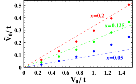
Figure 3: (Color online) The dots represent the renormalized impurity potential at the impurity site as a function of the bare impurity potential with the hole concentrations $x=0.05$ (blue), $0.125$ (green), and $0.2$ (red). The broken lines are $g_{t}V_{0}$.

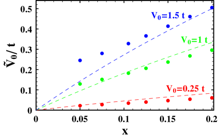
Figure 4: (Color online) The dots represent the renormalized impurity potential at the impurity site as a function of the hole concentration with the bare impurity potentials $V_{0}=0.25t$ (red), $1t$ (green), and $1.5t$ (blue). The broken lines are $g_{t}V_{0}$.

Note that $\tilde{V}_{0}$ is strongly suppressed and is quite close to $g_{t}V_{0}$, where $g_{t}$ is the Gutzwiller renormalization factor of the uniform system. These results agree with our VMC results in the previous section. Here, $\tilde{V}_{0}$ deviates upward from $g_{t}V_{0}$ when $V_{0}$ is large near the half filling. This is possibly related to the position dependence of $\tilde{V}_{i}$. Originally, the impurity potential is nonzero only at the impurity site. However, after solving the BdG equation, the renormalized impurity potential distributes more broadly as shown in Fig. 5. Namely, as $V_{0}$ becomes larger and $x$ becomes smaller, the renormalization effect reduces at the impurity site whereas it broadens toward the neighboring sites.

This broadening can be understood as follows: Basically, energy loss by the impurity potential reduces electron occupation at the impurity site. However, the hole prefers to move around to gain the kinetic energy. Therefore, to minimize the total energy, the $\delta$-function impurity potential is broadened by $\mu_{i}$. More explicitly, the contribution to $\mu_{i}$ from the kinetic energy contains a factor

$$\frac{dg^{t}_{ij}}{dx_{i}}=\sqrt{\frac{1}{2x_{i}(1+x_{i})^{3}}}\,\sqrt{\frac{2x_{j}}{1+x_{j}}},$$ (19)

which behaves as $\sqrt{x_{j}/x_{i}}$ near the half filling. Suppose the local hole densities behave as $x_{i}\sim x^{\delta_{i}}$, $x_{j}\sim x^{\delta_{j}}$ with some exponents $\delta_{i}$, $\delta_{j}$. Then, $dg^{t}_{ij}/dx_{i}\sim x^{(\delta_{j}-\delta_{i})/2}$ as $x\rightarrow 0$. If $\delta_{i}\neq\delta_{j}$, then $\mu_{i}$ or $\mu_{j}$ diverges and the self-consistent condition is not satisfied. Therefore, $\delta_{i}=\delta_{j}$, which tends to make the hole distribution more uniform.

Such extension of the impurity potential is also reported in the context of the unitary impurity potential by Poilblanc et al. Poilblanc94 and in the weak-coupling context by Ziegler et al. Ziegler96 In addition, Bulut Bulut00 and Ohashi Ohashi01 reported that the agreement between experimental data and the random-phase approximation is improved by adding phenomenological extended range potential.

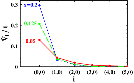
Figure 5: (Color online) The position dependence of the renormalized impurity potential for $V_{0}=1t$.

At half filling, the non-magnetic impurity potential should not affect the ground state because each site has to be occupied by one electron in any case. However, they do affect the ground-state energy. In the words of the BdG equation, the impurity potential is renormalized by $\mu_{i}$ in $H_{\rm BdG}$, and not in $E_{\rm GA}$. This is different from the well-known renormalization of the hopping and the exchange term described by $g^{t}_{ij}$ and $g^{s}_{ij}$; these renormalization factors influence both the ground state and the ground-state energy.

IV.2 Local density of states

The projected quasi-particle states $P^{\prime}\gamma_{\sigma n}^{\dagger}|\psi\rangle$ are approximately orthogonal to each otherFukushima08 . We regard them as excited states and calculate the density of states (DOS). Then, the local DOS (LDOS) is represented by

$$N(r,\omega)=g^{t}_{rr}\sum_{n}\left[|u_{r}^{n}|^{2}\delta(\omega-E_{n})+|v_{r}^{n}|^{2}\delta(\omega+E_{n})\right].$$ (20)

To obtain dense spectra, we use a supercell composed of 24$\times$24 sites whose origin has the impurity, and this supercell is repeated so as to construct a superlattice of 10$\times$10 supercells with the periodic boundary conditionTsuchiura00 . Then, the Hamiltonian can be block-diagonalized by the Fourier transform with respect to the supercell indices, and the calculation of expectation values is reduced to an average over many quasi-twisted boundary conditions of the 24$\times$24 site system. This supercell method is useful to obtain dense energy levels although it seems to overestimate correlation functions between very distant sites if the supercell size is too small and the number of supercells is too large. Except for this supercell boundary condition, the other conditions of the calculation are the same as those in Sec. IV.1. Since spectra in finite systems are discrete, we replace each $\delta$-function by the Gaussian distribution with the standard deviation $\delta E=0.02t$ to obtain continuous DOS.

Figure 6(a) shows the calculated LDOS at the impurity site as well as its nearest, second, and third neighbors. The DOS of the uniform system ($V_{0}=0$) is also plotted by dotted lines as a reference. Here, we have chosen $V_{0}=1t$ as the impurity potential, which is of the same order as the renormalized band width ($8g_{t}t$). Nevertheless, it is well screened by $\mu_{i}$ and the LDOS is not very site-dependent in agreement with results in Sec. IV.1. At the impurity site, the hole density is larger, and thus $g^{t}_{rr}$ is large. As a result the LDOS is also larger than those of the other sites. The peak at $E\sim-0.37t$ is the van Hove peak; the band renormalization by $g_{t}$ makes it closer to the Fermi surface. In fact, another van Hove peak appears in the positive bias at $E\sim 0.37t$. It is much weaker than the negative-bias van Hove peak, and only appears as a small shoulder of the the coherence peak in the resolution of Fig. 6(a). Some small portion of the original electron band around the van Hove peak is unoccupied in the mean-field superconducting ground state due to the electron-hole mixture. Even though that portion is small, the singular DOS enhances it to yield the positive-bias van Hove peak.

For comparison, we also show in Fig. 6(b) the results of the system without the strong correlation, i.e, let us set $g^{t}_{ij}=g^{s}_{ij}=1$ and $\mu_{i}=0$ in Eq. (15) and solve the BdG equation. $J$ and $\mu$ are determined in the same way as in the strongly correlated case, i.e., $4J\Delta_{ij}=0.3t$ for the uniform system. Here, we use supercells of $36\times 36$ sites to obtain dense spectra; if the same system size is used, energy level spacings are larger than those in the correlated systems due to the wider band width. The impurity potential is also $V_{0}=1t$. Note that it is this time much smaller than the band width $8t$. Nevertheless, comparing Figs. 6(a) and 6(b), it is clear that the system without strong correlation is much more disordered than the one with the correlation.

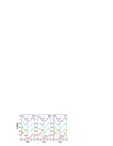
Figure 6: (Color online) The LDOS for one impurity system with $V=1t$ and $x=1/8$, at the impurity site and its nearest, second, and third neighbor, calculated by three different BdG equations: (a) with $g^{t}_{ij}$, $g^{s}_{ij}$, $\mu_{i}$, (b) without correlation ($g^{t}_{ij}=g^{s}_{ij}=1$, $\mu_{i}=0$), (c) without the local chemical potentialGarg08 (with $g^{t}_{ij}$, $g^{s}_{ij}$, but $\mu_{i}=0$). The dotted lines are the DOS in the uniform system ($V_{0}=0$) as a reference.

From Fig. 6(b), it is clear that the $\delta$-function potential makes the LDOS asymmetric.QHWangDHLee03 ; Nunner05 That is, some weight of the LDOS tends to move to the right at the impurity site, and to the left at the nearest neighbor site. The shift is large at high energy, and small at low energy. This asymmetry appears because the $\delta$-function potential lifts the degeneracy of two quasi-particles: (i) a linear combination between an electron state at site 1 and a hole state at site 2, or (ii) a linear combination between an electron state at 2 and a hole state at 1. We discuss it more in detail using a two-site system in Appendix A. With the strong correlation in Fig. 6(a), however, the asymmetry is less pronounced and the LDOS seems more symmetric. Most likely, the broadening of the impurity potential by $\mu_{i}$ results in weakening of the asymmetry.

IV.3 Comparison with other strongly-correlated BdG equations

IV.3.1 Importance of including the local chemical potential $\mu_{i}$

Garg et al. used a similar BdG equationGarg08 . Although the definition of the local renormalization factors is the same, they do not take into account the effective local chemical potential $\mu_{i}$ that minimize the total energy. They have reported that the spatially averaged LDOS shows protected V-shapes at low energy, and stated that the correlated systems are less disordered. For the testing purpose, we have also solved their BdG equation and show the resultant LDOS in Fig. 6(c). The parameters are the same as Fig. 6(a), and the uniform limits of these two BdG equations are identical. We have found that the LDOS before the spatial average is actually quite disordered, especially at the impurity site, and that the V-shaped LDOS appears only after the average. Therefore, it seems difficult to conclude that the LDOS in Fig. 6(c) is less disordered than the LDOS in Fig. 6 (b), in our opinion.

A more serious problem of their method appears in the local hole density as a function of the bulk hole density shown in Fig. 7. As already mentioned above, the non-magnetic impurity potential at half filling should not affect the ground state because each site has to be occupied by one electron in any case. Hence one can naturally imagine that the local hole density $x_{0}$ at the impurity site approaches the bulk hole density $x$ as $x\rightarrow 0$. However, if $\mu_{i}$ is not taken into account, $x_{0}-x$ increases as $x$ decreases. Therefore, it is questionable if the method by Garg et al. correctly captured the properties of the strongly correlated systems.

Figure 7: The relative hole density $x_{0}-x$ at the impurity site as a function of the bulk hole density $x$ solved for $V_{0}=0.25t$ by the two different BdG equations; without $\mu_{i}$Garg08 and with $\mu_{i}$.

Capello et al. Capello08 solved the BdG equation with extended Gutzwiller renormalization factors, but without the local chemical potential. Although we have not duplicated their results, we speculate that they have similar problems as Garg et al. because of the lack of the local chemical potential to minimize the total energy.

IV.3.2 Large $U$ instead of the Gutzwiller projection

Andersen and HirschfeldAndersen08 and some references therein used the BdG equation without the Gutzwiller renormalization factors ($g_{t}=g_{s}=1$). They took into account the electron correlation by the Hubbard $U$ term of the mean-field level. In that case, the screening effect similar to the one described in this paper can be obtained because $-Un_{i\bar{\sigma}}$ plays a role of our local chemical potential $\mu_{i}$. Since the impurity potential reduces electron occupation, the Coulomb energy loss is smaller there. Namely, summing up the potential and Coulomb energy loss, the total loss at the impurity site become less prominent by $U$. Note that, however, the strength of the screening depends on how one chooses $U$. A problem is that the mean-field decoupling of the $U$ term may underestimate the exchange energy and overestimate the kinetic energy especially near the half filling; the ground state would be strongly influenced by them.

IV.4 Smoothly varying impurity potential

As has been shown above, short-range impurity potential is screened by $\mu_{i}$. Accordingly, what remains must be the smooth variation in the potential. Here, we demonstrate the influence of the strong electron correlation on it using the Coulomb potential.

Instead of $H_{\rm imp}$, we consider the Coulomb potential from randomly located off-plane impurities, namely,

$$H_{\rm smooth}\equiv\sum_{r\sigma}V_{r}c_{r\sigma}^{\dagger}c_{r\sigma},$$ (21)

$$V_{r}\equiv\sum_{\ell=1}^{N_{\rm imp}}\frac{V_{\rm C}}{\sqrt{(r-r_{\ell})^{2}+d^{2}}},$$ (22)

where $N_{\rm imp}$ is the number of impurities, $r_{\ell}$ is the position of $\ell$-th impurity projected on the $xy$ plane, and $d$ is the off-plane distance. Here, we take $V_{\rm C}=1t$ and $d=1$ and adjust $\mu$ to satisfy $x=1/8$ simultaneously with the self-consistency condition. In addition, one supercell has 20$\times$20 sites with $N_{\rm imp}=12$ impurities, and the same impurity configuration is repeated so as to construct a superlattice of 10$\times$10 supercells. For simplicity, in determining the Coulomb potential in Eq. (22), we use only one of the cells, i.e., the system of 20$\times$20 sites with the periodic boundary condition.

Figure 8 shows the LDOS at 4 sites A, B, C, and D, each of which has a different hole concentration. The LDOS in hole-rich regions (e.g., A) has high coherence peaks with low gap energy. In contrast, hole-poor regions (e.g., D) has low coherence peaks with high gap energy. Figure 9 compares the spatial dependence of the bare impurity potential $V_{r}-N_{L}^{-1}\sum_{r}V_{r}$ and the renormalized impurity potential $\tilde{V}_{r}-N_{L}^{-1}\sum_{r}\tilde{V}_{r}$. Here, we have subtracted the spatial average of the potential. It is clear that the renormalized impurity potential has much smaller and smoother variation.

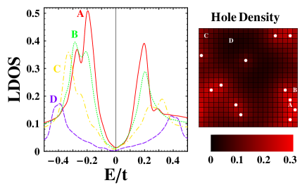
Figure 8: (Color online) (Left) The LDOS at 4 sites A, B, C and D indicated in the right figure, for the system with smoothly varying potential with $x=1/8$, $V_{\rm C}=1t$, $d=1$, $N_{\rm imp}=12$, and supercell size 20$\times$20 sites, solved by the Gutzwiller-projected BdG equation. (Right) The hole density distribution in a supercell. The white dots are positions of the impurities.

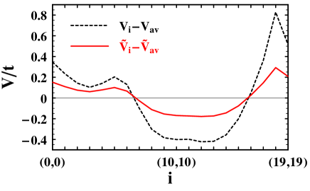
Figure 9: (Color online) Spatial dependence of the bare impurity potential $V_{i}-N_{L}^{-1}\sum_{i}V_{i}$ and the renormalized impurity potential $\tilde{V}_{i}-N_{L}^{-1}\sum_{i}\tilde{V}_{i}$ along a diagonal line (from the left bottom to the right top in the hole density plot of Fig. 8).

Nunner et al. Nunner05 pointed out for the conventional BdG equation with smoothly varying potential that the LDOS at site $r$ is similar to the DOS in the uniform system with shifted chemical potential $\tilde{\mu}=\mu-V_{r}$. This argument can be also applied to our system. However, the Gutzwiller renormalization factors make a difference in the relation among the hole density $x_{r}$, the gap energy, and the height of the coherence peaks. In the systems without the Gutzwiller projection, $\Delta_{ij}$ is determined by the DOS near the Fermi level. Namely, $\Delta_{ij}$ takes maximum when the chemical potential is at the van Hove singularity. Accordingly, when $\Delta_{ij}$ is large, the gap energy and the peak height are also large. In contrast, with the Gutzwiller renormalization factors, as $x\rightarrow 0$, (i) the band shrinks by $g^{t}_{ij}$ and thus the DOS near the Fermi level increases, and (ii) the pairing interaction is enhanced by $g^{s}_{ij}$. Because of (i) and (ii), $\Delta_{ij}$ and the gap energy monotonically increases as $x\rightarrow 0$. Furthermore, the LDOS contains an extra factor $g^{t}_{ii}$, and thus the peak height decreases as $x$ decreases.

Note that this anticorrelation between the gap energy and the peak height as well as the large gap distribution is consistent with the experiments Fang06 ; McElroySci05 . However, according to our calculation, the large spatial variation in the LDOS accompanies large variation in the hole density, which has yet to be verified by the experiments.

V Summary and discussion

In this paper, we have investigated the renormalization of the impurity potential by the strong correlation. The VMC calculation has shown that impurity potential scattering matrix elements between Gutzwiller-projected quasi-particle excited states are as strongly renormalized as the hopping terms. It may be understood by the Fourier transform of the $\delta$-function impurity potential having a form of the hopping term in $k$ space. The (real-space) hopping term is known to be renormalized by a factor less than unity because it is more difficult to hop in the presence of the double occupancy prohibition. Even in $k$ space, if electrons are densely packed in the lattice, it must be similarly difficult to hop from $k$ to $k^{\prime}\neq k$, then the impurity potential and the hopping term should be renormalized similarly.

Such reduction in the impurity potential is also seen by the BdG equation with local Gutzwiller renormalization factors. Near the half filling of the strongly correlated systems, the influence of the non-magnetic impurity potential on the ground state is small because each site has to be occupied by almost one electron in any case. However, the impurity potential does affect the ground-state energy. Such properties appear by taking into account effective local chemical potential, which is paid little attention to in the literature. In addition, the local chemical potential effectively broadens the impurity potential because holes prefer to move around to gain the kinetic energy. Effect of smoothly varying impurity potential has been briefly discussed. It shows large gap distribution. If the Gutzwiller renormalization factors are taken into account, the gap energy and the peak height are anticorrelated. These properties are consistent with the experiments Fang06 ; McElroySci05 .

In fair comparison, there are also some disagreements with the experiments. According to our results, short-range non-magnetic potential variations are reduced, thus the system is more uniform, and accordingly the $d$-wave superconductivity can be robust. However, in the experiments, the system seems quite disordered but still the $d$-wave is robust. Such short-range disorder may be introduced by spatial modulation of $t_{ij}$ or $J$, which can be enhanced by the strong correlation FukushimaSNS , or by magnetic impurities, or by the electron-lattice interaction CPChou09 .

In addition, although the smooth impurity potential variation yields anticorrelation between the gap energy and the peak height, it does not show the almost spatially independent V-shaped LDOS at low energy seen often in the experiments, which can be explained instead in the case of the rapid potential variationCPChou08 . In our previous paperCPChou08 , we have discussed the LDOS of stripe states, where $\Delta_{ij}$ contains two components; one is spatially uniform and the other is oscillating, typically with wave number $q=\pi/4$ or $\pi/2$. Then, the V-shaped gap is determined by the uniform component, and the oscillating component influences it little. As a result, the linear slope of V-shape is robust (it does not have much spatial dependence). This is rather counterintuitive because one may think that the local gap could be determined by $\Delta_{ij}$. However, the superconducting gap is not determined by such local properties, but by “coherence”, i.e., spatial dependence of $\Delta_{ij}$. Let us recall that, in the case of the zero-momentum pairing as the conventional BCS theory, the spin-up electron band couples with the spin-down hole band (upside-down spin-down electron band); these bands intersect at the Fermi level, and a gap opens by a nonzero superconducting order parameter. On the other hand, the oscillating components contain only pairing with nonzero center-of-mass momentum. Then, the spin-up electron band couples with the $q$-shifted (or multiples-of-$q$ shifted) spin-down hole band. The point is, these bands typically intersect not at the Fermi level except for limited points. In such cases, the V-shape of the LDOS is not affected a lot.

Similarly, oscillations of the variational parameters other than $\Delta_{ij}$ with wave number $q$ mix “the bare band” and “the bands shifted by multiples of $q$”. Such terms change the band structure especially near band intersections. However, this change in the band structure is not related to the superconductivity, at least in the mean-field approximation. The superconducting DOS depends on where one puts the chemical potential, but general properties near the V-shaped LDOS is determined by $\Delta_{ij}$.

The smooth impurity potential variation considered in Sec. IV.4 is similar to the stripe states with $q\simeq 0$. Since $q$ is small, the oscillating components of $\Delta_{ij}$ has effect similar to the uniform component $q=0$. Namely, it affects every state at the Fermi level. However, the gap has now spatial dependence because $q$ is not completely zero. In this case, the local gap is determined by $\Delta_{ij}$; the LDOS at sites $i$ is similar to the DOS in the uniform system with $\tilde{\Delta}^{x}=-\tilde{\Delta}^{y}=\Delta_{i,i+\hat{x}}$, $\tilde{\chi}=\chi_{ij}$, and $\tilde{\mu}=\mu-V_{i}$. Therefore, there is nothing like the “uniform component” in the argument of the stripe state, and thus the linear slope of V-shape in the LDOS is not robust anymore. This issue will be addressed in the future.

Appendix A LDOS asymmetry caused by $\delta$-function potential

As shown in Fig. 6, the $\delta$-function potential causes asymmetry in the LDOS near the impurity site. Such asymmetry may be important because some STM experiments analyze data by taking the ratio between intensities of positive and negative bias Kohsaka07 : the symmetric part of the LDOS is canceled and its asymmetric part remains. To explain the origin of the asymmetry, let us diagonalize the BdG Hamiltonian of a simple two-site problem analytically in the following. We know that it is not realistic to apply the mean-field approximation to two-site problems. However, it provides us some insight into numerical solutions in the bulk systems.

Suppose the potentials at sites 1 and 2 are $V$ ($>0$) and $-V$, respectively. By putting the states in the order of electrons ${1\uparrow}$, ${2\uparrow}$, and holes ${1\downarrow}$, ${2\downarrow}$, the BdG Hamiltonian matrix is written as

$$H_{\rm 2site}=\begin{pmatrix}V&-t&0&\Delta\\ -t&-V&\Delta&0\\ 0&\Delta&-V&t\\ \Delta&0&t&V\end{pmatrix}.$$ (23)

Let us start from a simple case of $t=0$ and assume $V<\Delta$. Then, $\Delta$ mixes ${1\uparrow}$ electron and ${2\downarrow}$ hole with the equal weights. We call the linear combination of them with positive and negative energy the quasi-particle A⁺ and A^-, respectively. Similarly, B^± denotes the linear combination of ${2\uparrow}$ electron and ${1\downarrow}$ hole with positive/negative energy.

If $V=0$, A and B are degenerate. Finite but small $V$ causes energy difference between A and B, namely, $E_{{\rm A}^{\pm}}=\pm\Delta+V$, $E_{{\rm B}^{\pm}}=\pm\Delta-V$. In the ground state, A^- and B^- are occupied, but A⁺ and B⁺ are unoccupied. First we focus on 1$\uparrow$. Then, the electron addition spectrum is at $E=E_{{\rm A}^{+}}$, the removal is at $E=E_{{\rm A}^{-}}$. Namely, the finite V just shifts the whole spectra by $V$, and the local spectra are not symmetric around $E=0$. On the other hand, the spectra of site 2 shift by $-V$. As a result, the spectra summed over sites 1 and 2 are still symmetric. As for 1$\downarrow$, the addition is at $-E_{{\rm B}^{-}}=E_{{\rm A}^{+}}$, and the removal is at $-E_{{\rm B}^{+}}=E_{{\rm A}^{-}}$ (these negative signs originate from the treatment of 1$\downarrow$ as a hole), which are identical to the spectra of 1$\uparrow$ as expected.

Next, let us consider $t\neq 0$. Then, $t$ mixes A⁺ and B^-, and the eigenstates are linear combinations of them whose eigenenergies are $\pm[t^{2}+\left(\Delta+V\right)^{2}]^{1/2}$. The eigenenergies of superposition of A^- and B⁺ are $\pm[t^{2}+\left(\Delta-V\right)^{2}]^{1/2}$. As $t$ increases, the LDOS asymmetry becomes weaker, but it never disappears.

Back to the bulk systems, maybe we can physically explain the asymmetry as follows. Since $J$ term causes pairing, a Cooper pair is formed more or less between nearest neighbors (site 1,2) when a snapshot is taken. This Cooper pair is a resonance of “states where sites 1 and 2 are occupied by electrons” and “states where both are occupied by holes”. Destruction of the pair leaves a quasi-particle. There are two possibilities for it; (i) an “electron at site 1 and hole at site 2”, and (ii) an “electron at 2 and hole at 1”. The $\delta$-function potential lifts the degeneracy of these quasi-particles. That results in the asymmetry in the local spectra although the bulk spectra are symmetric as in the two-site problem above. In the bulk system, the spectra are continuous, and the spectral shift by the impurity potential is larger at high energy than at low energy because (i) the near-nodal quasi-particles at low energy are less influenced by the impurity potential because there are not many states to mix with, and (ii) the shift is caused by $\Delta$ and it is smaller at lower energy.

References

- (1) P. W. Anderson, J. Phys. Chem. Solids 11 26 (1959).
- (2) A. N. Pasupathy, et al., Science 320, 196 (2008).
- (3) K. McElroy, et al., Phys. Rev. Lett. 94, 197005 (2005).
- (4) X. J. Zhou, et al., Phys. Rev. Lett. 92, 187001 (2004).
- (5) K. M. Shen, et al., Science 307, 901 (2005).
- (6) A. C. Fang, L. Capriotti, D. J. Scalapino, S. A. Kivelson, N. Kaneko, M. Greven, and A. Kapitulnik, Phys. Rev. Lett. 96 017007 (2006).
- (7) Y. Kohsaka et al., Science 315 1380 (2007).
- (8) P. W. Anderson, Science 288 480 (2000).
- (9) A. Garg, M. Randeria, N. Trivedi, Nature Phys. 4, 762 (2008).
- (10) N. Fukushima, C.-P. Chou, T. K. Lee, J. Phys. Chem. Solids 69, 3046 (2008).
- (11) Q.-H. Wang, Z.D. Wang, Y. Chen and F.C. Zhang, Phys. Rev. B 73, 092507 (2006).
- (12) C. Li, S. Zhou, and Z. Wang, Phys. Rev. B 73 060501(R) (2006).
- (13) N. Fukushima, Phys. Rev. B 78, 115105 (2008).
- (14) H. Alloul, J. Bobroff, M. Gabay, P. J. Hirschfeld, Rev. Mod. Phys. 81, 45 (2009).
- (15) Y. Chen and C. S. Ting, Phys. Rev. Lett. 92, 077203 (2004).
- (16) J. W. Harter, B. M. Andersen, J. Bobroff, M. Gabay, and P. J. Hirschfeld, Phys. Rev. B 75, 054520 (2007).
- (17) H. Tsuchiura, Y. Tanaka, M. Ogata, and S. Kashiwaya, Phys. Rev. B 64, 140501(R) (2001).
- (18) M. Ogata and A. Himeda, J. Phys. Soc. Jpn. 72, 374 (2003).
- (19) Z. Wang and P. A. Lee, Phys. Rev. Lett. 89, 217002 (2002).
- (20) M. Gabay, E. Semel, P. J. Hirschfeld, and W. Chen, Phys. Rev. B 77, 165110 (2008).
- (21) S.-D. Liang and T. K. Lee, Phys. Rev. B 65, 214529 (2002).
- (22) Q.-H. Wang and D.-H. Lee, Phys. Rev. B 67, 020511(R) (2003).
- (23) T.S. Nunner, B.M. Andersen, A. Melikyan, and P.J. Hirschfeld, Phys. Rev. Lett. 95, 177003 (2005).
- (24) B. M. Andersen and P. J. Hirschfeld, Phys. Rev. Lett. 100, 257003 (2008).
- (25) W. Ziegler, H. Endres, and W. Hanke, Phys. Rev. B 58, 4362 (1998).
- (26) K. McElroy et al., Science 309, 1048 (2005).
- (27) C.-P. Chou, T. K. Lee, and C.-M. Ho, J. Magn. Magn. Mater. 310, 474 (2007).
- (28) C.-P. Chou, T. K. Lee, C.-M. Ho, Phys. Rev. B 74, 092503 (2006).
- (29) F. C. Zhang, C. Gros, T. M. Rice, H. Shiba, Supercond. Sci. Technol. 1, 36 (1988).
- (30) D. Poilblanc, D. J. Scalapino, and W. Hanke, Phys. Rev. B 50, 13020 (1994).
- (31) W. Ziegler, D. Poilblanc, R. Preuss, W. Hanke, D. J. Scalapino, Phys. Rev. B 53, 8704 (1996).
- (32) N. Bulut, Phys. Rev. B 61, 9051 (2000).
- (33) Y. Ohashi, J. Phys. Soc. Jpn. 70, 2054 (2001).
- (34) H. Tsuchiura, Y. Tanaka, M. Ogata, and S. Kashiwaya, Phys. Rev. Lett. 84, 3165 (2000).
- (35) M. Capello, M. Raczkowski, and D. Poilblanc, Phys. Rev. B 77, 224502 (2008).
- (36) C.-P. Chou and T. K. Lee, in preparation.
- (37) C.-P. Chou, N. Fukushima, and T. K. Lee, Phys. Rev. B 78, 134530 (2008).