Multi-Cut Solutions of Laplacian Growth

Abstract

A new class of solutions to Laplacian growth (LG) with zero surface tension is presented and shown to contain all other known solutions as special or limiting cases. These solutions, which are time-dependent conformal maps with branch cuts inside the unit circle, are governed by a nonlinear integral equation and describe oil fjords with non-parallel walls in viscous fingering experiments in Hele-Shaw cells. Integrals of motion for the multi-cut LG solutions in terms of singularities of the Schwarz function are found, and the dynamics of densities (jumps) on the cuts are derived. The subclass of these solutions with linear Cauchy densities on the cuts of the Schwarz function is of particular interest, because in this case the integral equation for the conformal map becomes linear. These solutions can also be of physical importance by representing oil/air interfaces, which form oil fjords with a constant opening angle, in accordance with recent experiments in a Hele-shaw cell.

I Introduction

Background and motivation: The Laplacian growth (LG) is a free boundary motion governed by gradient of a harmonic field. It describes numerous physical processes GH with a moving boundary between two immiscible phases (an interface) far from equilibrium and profoundly interconnects various branches of mathematical physics KMWZ; Gust. LG in two dimensions is of special importance since in the zero surface tension limit it has a remarkably rich integrable structure Richardson; MWZ; KKMWZ and an impressive list of exact solutions in the form of conformal maps with pole Kuf; SB84; M90 and logarithmic H86; BP86; MS94; SM94 time-dependent singularities (many of these solutions cease to exist in a finite time due to the interface instability.) In addition, there exist a family of explicit solutions BAmar; Tu; AMZ with time-independent branch cuts with fixed endpoints which describe growth of self-similar air ‘fingers’ in a wedge geometry (or in the plane with the rotational $\mbox{$\mathbb{Z}$}_{N}$-symmetry imposed).

Do other solutions exist, apart from those mentioned above? Answering ‘yes’ to this question, we hereby present a new family of conformal maps with time-dependent cuts, study their dynamics and provide examples. This family is the most general solution to the LG problem (in the absence of surface tension) which can be written in terms of analytic functions. All rational, logarithmic and self-similar solutions known so far (and mentioned above) are shown to be special or limiting cases of these newly found ones.

In this paper we consider a simply connected exterior 2D LG problem with a source/sink at infinity. In the context of Hele-Shaw flows Hele-Shaw1898 (the prototype of all 2D LG processes RMP86), it corresponds to a finite bubble of an inviscid fluid (air) surrounded by a viscous fluid (oil) with a source or sink at infinity. In what follows we hold to this hydrodynamic interpretation.

The standard formulation of the exterior LG problem in 2D planar geometry is as follows:

$$\!\!\left\{\begin{array}[]{l}\left.\begin{array}[]{l}{\bf v}=-{\bf\nabla}p\\ \Delta p=0\end{array}\right\}\mbox{in }D(t)\\ \left.\begin{array}[]{l}p=\mbox{const}\\ V_{n}=-\partial_{n}p\\ \end{array}\right\}\mbox{at }\Gamma(t)\\ p(x,y)=-\frac{Q}{2\pi}\log R\mbox{, when }R=\sqrt{x^{2}+y^{2}}\to\infty.\\ \end{array}\right.$$ (1)

Here $t$ is time, $\Gamma(t)$ is the boundary (an oil/air interface) of an infinite planar domain $D(t)$ containing infinity and filled with oil, $p$ is the pressure field, ${\bf v}$ is velocity of oil, $V_{n}$ is normal velocity of the oil/air interface, $\partial_{n}$ stands for normal derivative at the interface, and $Q$ is a pumping rate assumed to be time-independent (positive for the suction problem and negative for the injection one).

The first equation in the system (1) is the Darcy law in scaled units, which determines the local velocity of oil in the Hele-Shaw cell. The second equation follows from continuity and incompressibility of oil, $\mbox{div}\,{\bf v}=0$. The third equation results from the fact that in fluids with negligible viscosity pressure is the same everywhere in the fluid, $p=\mbox{const}$, so, neglecting surface tension, one can set $p$ to be the same constant along both sides of the interface. The fourth equation states that normal velocity of fluid at the interface and that of the interface itself coincide (continuity). The last equation gives the asymptotic of $p$ far away from the interface in the presence of a single sink of strength $Q$ placed at infinity.

A reformulation of the LG problem in terms of complex variables and analytic functions is particularly instructive. We conclude the introduction by a brief review of the time-dependent conformal map approach.

The conformal map formulation. Let us introduce a time-dependent conformal map, $z=f(w,t)$, from the exterior of the unit circle, $|w|\geq 1$, in an auxiliary mathematical $w$-plane to the domain $D(t)$ occupied by oil in the physical plane $z=x+iy$. Then the interface at time $t$ is a closed curve swept by $f(e^{i\phi},t)$ as $\phi$ runs from $0$ to $2\pi$. Below we sometimes do not indicate the time dependence explicitly and write simply $f(w)$. It is convenient to normalize the conformal map by the condition that $\infty$ is mapped to $\infty$ and the derivative at infinity is a real positive number $r$ (the conformal radius), so that the Laurels expansion at infinity has the form

$$f(w)=rw+u_{0}+u_{1}/w+u_{2}/w^{2}+\ldots$$ (2)

(the coefficients $u_{i}$ are in general complex numbers).

It is well known Galin; PK45 that the LG dynamics of the interface is equivalent to the following equation for $f(e^{i\phi},t)$:

$${\rm Im}(\bar{f}_{t}f_{\phi})=\frac{Q}{2\pi},$$ (3)

where subscripts stand for partial derivatives and a bar for complex conjugation. This nonlinear equation is remarkable because it possesses an infinite number of conservation laws Richardson and an impressive list of non-trivial solutions with moving singularities Kuf; SB84; M90; H86; BP86; MS94; SM94, which are either poles or logarithmic branch points lying strictly inside the unit circle. In all these cases the conformal map $f(w)$ thus admits an analytic continuation across the unit circle, so the function $f(w)$ is actually analytic not only in its exterior but in some larger infinite domain containing it. Assuming that $f(w,t)$ is analytically extendable across the unit circle for all $t$ in some time interval, one can analytically continue the LG equation (3) itself. Set $\bar{f}(1/w,t)\equiv\overline{f(1/\bar{w},t)}$, then equation (3) can be rewritten as

$$\partial_{w}f(w,t)\partial_{t}\bar{f}(1/w,t)-\partial_{t}f(w,t)\partial_{w}\bar{f}(1/w,t)=1/w$$ (4)

(we have set $Q=\pi$ that means a resealing of time units). Under our assumption the functions $f(w,t)$ and $\bar{f}(1/w,t)$ have a common domain of analyticity containing the unit circle $|w|=1$, and $w$ in equation (4) is supposed to belong to this domain. In fact, for rational and logarithmic solutions, this equation holds everywhere in the $w$-plane except for poles and branch cuts of $f(w,t)$ and $\bar{f}(1/w,t)$. We note in advance that the general multi-cut solutions constructed below have the same property. Namely, the functions $f(w,t)$ and $\bar{f}(1/w,t)$ have a common domain of analyticity where they actually solve the analytically continued LG equation (4) and not just (3).

As said earlier, there are also self-similar $\mbox{$\mathbb{Z}$}_{N}$-symmetric solutions BAmar; Tu; Gust; AMZ containing a time-independent fractional power singularity which corresponds to the interface self-intersection point at the origin. In this case the analytic continuation is possible through every point on the unit circle except those that are mapped to the origin. Again, the functions $f(w,t)$ and $\bar{f}(1/w,t)$ have a non-empty common domain of analyticity and equation (4) is valid everywhere in this domain.

II The Schwarz Function and Integrals of Motion

It is known Richardson; H86; H92; MS94; KMWZ; MWZ that the partial differential equation (4) can be integrated in terms of the Schwarz function. It is an analytic function, $S$, which connects $f(w)$ and $\bar{f}(1/w)$ in their common domain of analyticity: $\bar{f}(1/w)=S(f(w))$. Equivalently, the Schwarz function for a curve $\Gamma$ is an analytic function $S(z)$ such that $\bar{z}=S(z)$ for $z\in\Gamma$ Davis. In other words, $S(z)$ is an analytic continuation of the function $\bar{z}$ away from the curve. For analytic curves this function is known to be well defined in a strip-like neighborhood of the curve. If the curve depends on time, so does its Schwarz function, $S=S(z,t)$.

In terms of the Schwarz function the (analytically continued) LG equation (4) reads H92

$$S_{t}=\partial_{z}\log w$$ (5)

where $w=w(z,t)$ is the function inverse to the $f(w,t)$. Since $\partial_{z}\log w(z)$ is analytic everywhere in the oil domain $D(t)$, both sides of equation (5) are free of singularities there. Therefore, all singularities of $S(z,t)$ located in $D(t)$ are time-independent. Equivalently, the function

$$S_{+}(z)=\oint_{\Gamma(t)}\,\frac{S(\zeta)}{\zeta-z}\,\frac{d\,\zeta}{2\pi i}$$ (6)

defined for $z$ outside $D(t)$ by the integral of Cauchy type (where the integration contour $\Gamma$ has the standard anti-clockwise orientation) and analytically continued to $D(t)$ is constant in time: $\partial_{t}S_{+}(z,t)=0$. This implies conservation of harmonic moments $t_{k}$ Richardson which are coefficients of the Taylor expansion of $S_{+}(z)$ at $z=0$:

$$t_{k}=\frac{1}{2\pi ik}\oint_{\Gamma(t)}\frac{\bar{z}dz}{z^{k}}=$$

$$-\frac{1}{\pi k}\int_{D(t)}\frac{dx\,dy}{z^{k}},\qquad k=1,2,3,\dots,$$ (7)

where we assume, without loss of generality, that the contour $\Gamma(t)$ encircles the origin. In particular, $t_{1}=S_{+}(0)$. Besides, it is easy to see that the physical time $t$ is equal to the area of the air bubble divided by $\pi$:

$$t=\oint_{\Gamma(t)}\frac{\bar{z}\,dz}{2\pi i}$$ (8)

Thus the LG dynamics is a process such that the area surrounded by the interface grows linearly with time while the harmonic moments (7) (or the $S_{+}$-part of the Schwarz function (6)) are kept constant. It is important to note that the function $S_{+}$ (i.e., the infinite set of harmonic moments $t_{k}$) together with the variable $t$ fix the whole Schwarz function $S$ uniquely, at least locally in the variety of closed analytic contours in the plane. In a certain sense (made more precise in KMZ05), these data serve as local coordinates in the infinite dimensional variety of contours.

It is also worthwhile to mention that the function $S_{-}(z)=S(z)-S_{+}(z)$ is analytic in $D(t)$ and vanishes at infinity as $O(1/z)$ with the residue

$$\mbox{res}_{\infty}\,[S_{-}(z)dz]=-t$$ (9)

(the residue at infinity is defined as $\mbox{res}_{\infty}[dz/z]=-1$). The decomposition of the Schwarz function $S=S_{+}+S_{-}$ appears to be very useful. As it follows from properties of Cauchy-type integrals, the function $S_{-}(z)$ is given by the same integral (6) (with the opposite sign), where $z$ now belongs to $D(t)$.

The conformal map and the Schwarz function are connected in the following way:

$$\left\{\begin{array}[]{l}S(z)=\bar{f}(1/w)\\ z=f(w)\end{array}\right.$$ (10)

These formulas make it clear that if the functions $f(w)$ and $\bar{f}(1/w)$ have a common domain of analyticity containing the unit circle, then the Schwarz function is well-defined. They also imply the one-to-one correspondence between singularities of the function $f(w)$ inside the unit disk and singularities of the function $S(z)$ in $D(t)$ (which, by the properties of the Cauchy type integrals, are the same as singularities of the function $S_{+}(z)$).

Let us illustrate the one-to-one correspondence between singularities of $f(w)$ and $S_{+}(z)$ by the example of poles in which case it is especially transparent. Suppose that the conformal map $f(w)$ has a pole of order $k$ at a point $a$ inside the unit disk, so that the local behavior of $f$ near $a$ is

$$f(w)=\frac{A}{(w-a)^{k}}\,\,\,+\,\,\,\mbox{less singular terms}.$$ (11)

Then the function $S=\bar{f}(1/w)$ has a pole of the same order at the point $w=1/\bar{a}$:

$$S=\bar{f}(1/w)=\frac{\bar{A}}{(w^{-1}-\bar{a})^{k}}\,\,\,+\,\,\,\mbox{less singular terms}.$$ (12)

Because the point $1/\bar{a}$ together with its small neighborhood lies outside the unit disk (where $f$ is conformal), we can linearize the denominator in (12) near $z=f(1/\bar{a})$ and obtain

$$S(z)=\bar{A}\left[\frac{f_{\bar{a}}(1/\bar{a})}{z-f(1/\bar{a})}\right]^{k}\,\,\,+\,\,\,\mbox{less singular terms}$$ (13)

(here $f_{\bar{a}}(1/\bar{a})\equiv\partial_{w}f(1/w)$ at $w=\bar{a}$). Thus $S(z)$ necessarily has a singularity at $z=f(1/\bar{a})$ of the same type as $f(w)$ has at $w=a$.

Now we are ready to outline the general strategy of integration of the LG problem. Taken initial data, i.e., a conformal map $f(w)$ at $t=t_{0}$, one finds $S_{+}$ from (6) by rewriting it as integral over the unit circle in the mathematical plane:

$$S_{+}(z)=\frac{1}{2\pi i}\oint_{|w|=1}\frac{\bar{f}(1/w)\,df(w)}{f(w)-z}\,.$$ (14)

In order to obtain the LG dynamics, one then should solve the inverse problem: given the $S_{+}(z)$ and time $t$, to recover the conformal map $f(w,t)$. The last step is a part of the inverse potential problem and thus is hard to implement in general. Formally, this is equivalent to a nonlinear integral equation which is easy to derive using the definition of the Schwarz function in the form $f(\zeta)=\bar{S}(\bar{f}(1/\zeta))$. Integrating both sides of this equality with the Cauchy kernel $1/(w-\zeta)$ over the unit circle assuming that $|w|>1$, and using the fact that the $S_{-}$-part of the Schwarz function does not contribute to the integral, we get the integral equation

$$f(w)=rw+u_{0}+\frac{1}{2\pi i}\oint_{|\zeta|=1}\!\!\!\!\!\!\!\!\frac{\bar{S}_{+}(\bar{f}(1/\zeta))d\zeta}{w-\zeta},\quad|w|>1.$$ (15)

The same procedure at $|w|<1$ gives a “complimentary” equation

$$rw+u_{0}=\frac{1}{2\pi i}\oint_{|\zeta|=1}\!\!\!\!\!\!\!\!\frac{\bar{S}_{+}(\bar{f}(1/\zeta))d\zeta}{\zeta-w}+\bar{S}_{-}(\bar{f}(1/w)),\,|w|<1.$$ (16)

As their direct consequence, we can write the following useful formulae for the coefficients of the Laurels series (2):

$$u_{j}=\frac{1}{2\pi i}\oint_{|\zeta|=1}\bar{S}_{+}(\bar{f}(1/\zeta))\zeta^{j-1}d\zeta\,,\quad j\geq 0\,,$$ (17)

$$r=\frac{1}{2\pi i}\oint_{|\zeta|=1}\bar{S}_{+}(\bar{f}(1/\zeta))\zeta^{-2}d\zeta+\frac{t}{r}$$ (18)

Substituting them back into (2) and using (15), we get a set of integral equations

$$f(w)=rw+\sum_{j=0}^{d}u_{j}w^{-j}+$$

$$\frac{1}{2\pi i}\oint_{|\zeta|=1}\frac{\zeta^{d}\bar{S}_{+}(\bar{f}(1/\zeta))d\zeta}{w^{d}(w-\zeta)},\qquad|w|>1.$$ (19)

for any $d=-1,0,1,2,\ldots$. Being taken together with (17), all of them are equivalent to the original equation (15) which is reproduced at $d=0$. However, depending on the type of singularities of the function $S_{+}$, one or another form may be more convenient than others. The choice $d=-1$ gives an equation where none of the coefficients $u_{j}$ enter explicitly:

$$f(w)=rw+\frac{1}{2\pi i}\oint_{|\zeta|=1}\frac{w\bar{S}_{+}(\bar{f}(1/\zeta))d\zeta}{\zeta(w-\zeta)}\,,|w|>1.$$ (20)

This equation combined with relation (18) accomplishes integration of the LG problem. Let $f(w)=f(w|r)$ be a solution to equation (20) depending on the parameter $r$, then the time dependence is found from (18) which determines $r$ as an implicit function of $t$:

$$t=r^{2}-\frac{r}{2\pi i}\oint_{|\zeta|=1}\bar{S}_{+}(\bar{f}(\zeta|r))d\zeta$$ (21)

Alternatively, one may use the relation

$$t=\frac{1}{2\pi i}\oint_{|w|=1}\bar{f}(1/w)\,df(w)$$ (22)

leading to the same results.

In principle, this scheme provides a general solution to the LG problem but in a rather implicit form. However, for several important classes of functions $S_{+}(z)$ it can be made more explicit. In all effectively solvable cases, the r.h.s. of the integral equation simplifies drastically after shrinking the integration contour to singularities of the function $\bar{S}_{+}(\bar{f}(1/\zeta))$ inside the unit disk. Some examples are given in the next section.

III Rational and Logarithmic Solutions

In this section we apply the general method based on equations (20), (21) to construction of LG solutions with poles and logarithmic singularities.

III.1 Rational Solutions

By rational solutions we mean solutions to equation (4) whose only singularities are poles inside the unit disk (not mentioning a simple pole at infinity). The very fact that the rational ansate is consistent with the LG equation, i.e., that the number of poles is conserved and singularities of other types are not generated, is a consequence of the integral equation (15).

Let us take $S_{+}$ to be a rational function of a general form

$$S_{+}(z)=\sum_{m=1}^{N}\,\sum_{k=1}^{K_{m}}\frac{T_{m,k}}{(z-z_{m})^{k}}+\,T_{0,0}+\,\sum_{k=1}^{K_{0}}T_{0,k}z^{k}$$ (23)

where all the poles $z_{m}$ are in $D(t)$ and $T_{m,k}$ are arbitrary complex constants. Then the function $\bar{S}_{+}(\bar{f}(1/\zeta))$ has a pole at $0$ of order $K_{0}$ and poles of orders $K_{m}$ at the points $a_{m}$ such that $z_{m}=f(1/\bar{a}_{m})$ and does not have other singularities inside the unit disk. For convenience, we set $a_{0}=0$. Therefore, the integral in the r.h.s. of (15) is equal to the sum of residues at these poles. Calculating the residues, we obtain an expression for the conformal map in the form of a rational function of $w$ with poles of orders not higher than $K_{m}$ at the points $a_{m}$ inside the unit disk:

$$f(w,t)=r(t)w+u_{0}(t)+\sum_{m=0}^{N}\,\sum_{k=1}^{K_{m}}\frac{A_{m,k}(t)}{(w-a_{m}(t))^{k}},$$ (24)

The pole at $a_{0}=0$ is distinguished among the others because it does not move. All other poles as well as all coefficients depend on time. The coefficients $A_{m,k}$ are expressed through derivatives of the function $\bar{f}(1/w)$ at $w=a_{m}$. The general formulae are quite complicated. In fact what we really need are inverse formulae which express the integrals of motion $T_{m,k}$ through time-dependent coefficients of $f(w,t)$. Obviously,

$$T_{m,k}=\mbox{res}_{z_{m}}\left[(z-z_{m})^{k-1}S_{+}(z)dz\right]\,,\quad m\neq 0\,,$$

and the function $S_{+}(z)$ here can be substituted for the $S(z)$ because $S_{-}(z)$ is regular in $D(t)$. Passing then to the mathematical plane, we obtain the full list of constants of motion:

$$z_{m}\,=f(1/\bar{a}_{m}(t),t)\,,\quad m\neq 0$$ (25)

$$T_{m\not=0,k}=\mbox{res}_{\bar{a}^{-\!1}_{m}\!(t)}\left[(f(w,t)\!-\!z_{m})^{k-1}\bar{f}(w^{-1}\!\!,t)df(w,t)\right]$$

$$T_{0,k}\,=-\,\mbox{res}_{\infty}\left[(f(w,t))^{-k-1}\bar{f}(1/w,t)df(w,t)\right].$$

We note that $T_{m,k}$ have the meaning of “Whitham times” for a general Whitham hierarchy which covers the LG problem with zero surface tension. Each Whitham time $T_{m,k}$ is “coupled” to its own type of singularity. From this point of view, formulae (25) are relations of the hodograph type which provide a solution of the full genus zero Whitham hierarchy in an implicit form Krichever94.

Algebraic equations (25) express time-dependent parameters $r(t)$, $u_{0}(t)$, $a_{m}(t)$ and $A_{m,k}(t)$ implicitly via the constants of motion $z_{m}$ and $T_{m,k}$. To obtain a complete set of relations, we also need the equation (22) containing time $t$ explicitly. In our case the integral is reduced to a sum of residues:

$$t=-\mbox{res}_{\infty}[\bar{f}(w^{-1},t)df(w,t)]-\sum_{m}\mbox{res}_{\bar{a}^{-\!1}_{m}(t)}[\bar{f}(w^{-1},t)df(w,t)]$$

Comparing with (25) at $k=1$, we see that the residues at $1/\bar{a}_{m}$ are just constants $T_{m,1}$. Therefore,

$$t=-\mbox{res}_{\infty}[\bar{f}(1/w,t)df(w,t)]-\sum_{m}T_{m,1}.$$ (26)

So, we have $N+K+1$ complex algebraic equations, where $K=\sum_{m=0}^{N}K_{m}$, and one real algebraic equation for $N+K+1$ complex parameters and one real parameter which determine them as functions of time and $N+K+1$ constants of motion. Given initial conditions in the form (23), a solution to this system allows one to recover the time-dependent conformal map, according to the strategy outlined at the end of Section II.

In some important particular cases the general expressions given above become simpler and more explicit. For example, if none of the poles $a_{m}$ lies at the origin (i.e., $A_{0,k}=0$ for all $k\geq 1$), then $T_{0,k}=0$ for $k\geq 1$, $T_{0,0}=f(0,t)$ and

$$t=r(t)\bar{f}^{\prime}(0,t)-\sum_{m}T_{m,1},$$ (27)

(here $f^{\prime}(0,t)$ is the derivative of $f(w,t)$ at $w=0$). If, moreover, all poles in (24) are simple and none of them lies at the origin ($K_{m}=1$ for $m\neq 0$ and $K_{0}=0$), then the expressions for $T_{m,1}$ and $t$ acquire an especially compact and explicit form:

$$T_{m,1}=\left.\bar{A}_{m,1}(t)\partial_{w}f(1/w,t)\right|_{w=\bar{a}_{m}(t)}=$$

$$\bar{A}_{m,1}(t)\,\left(-\frac{r(t)}{\bar{a}_{m}^{2}(t)}+\sum_{l}\frac{A_{l,1}(t)}{(1-a_{l}(t)\bar{a}_{m}(t))^{2}}\right),$$ (28)

$$t=r(t)\bar{f}^{\prime}(0,t)-\sum_{m}T_{m,1}=$$

$$r^{2}(t)+\sum_{l,m}\frac{A_{l,1}(t)\bar{A}_{m,1}(t)}{(1-a_{l}(t)\bar{a}_{m}(t))^{2}}.$$ (29)

III.2 Logarithmic Solutions

For the class of logarithmic solutions, the function $S_{+}$ is taken in the form

$$S_{+}(z)=t_{1}+\sum_{m=1}^{N}\bar{A}_{m}\log\left(1-\frac{z}{z_{m}}\right)\,,$$ (30)

where all the branch points $z_{m}$ are in $D(t)$ and $t_{1}$, $A_{m}$ are arbitrary complex constants (note that this $t_{1}$ is the first harmonic moment from (7)). If

$$A_{0}=-\sum_{m=1}^{N}A_{m}\,\neq 0\,,$$

then there is also a branching at infinity. This function is multi-valued and one should fix a single-valued branch. In a neighborhood of the origin, we define it by the condition that $S_{+}(0)=t_{1}$. In order to continue it unambiguously to $D(t)$, it is necessary to introduce a system of cuts connecting all the branch points in such a way that the domain $D(t)\setminus\{\mbox{all cuts}\}$ be simply connected. There are many ways to draw the cuts. Although all of them are ultimately equivalent, it would be convenient for us to meet some requirements natural for the growth problem: to respect the democracy among the branch points $z_{m}$ and to ensure that the cuts always remain in $D(t)$. For the former, let us fix a point $q$ in $D(t)$ and make cuts from $q$ to all $z_{m}$ (and, if necessary, to infinity). For the latter, it is natural to choose $q=\infty$ since $\infty$ is the only point in $D(t)$ which remains there forever irrespectively of initial conditions. So, we fix a system of (non-intersecting) cuts from the points $z_{m}$ to $\infty$. Note that this choice of cuts implies that $S_{+}(z)$ does not have a definite value at $z=\infty$, even if $\infty$ is a regular point, because the limit depends on a particular way of tending $z\to\infty$.

Reconstructing $f$ from (15) in a similar way as for rational solutions, we introduce the points $a_{m}$ such that $f(1/\bar{a}_{m})=z_{m}$ inside the unit disk and notice that the integral in (15) is shrunk to residues of the differential

$$d\bar{S}_{+}(\bar{f}(1/\zeta))=\sum_{m=1}^{N}A_{m}d\log(\bar{f}(1/\zeta)-\bar{f}(1/a_{m}))$$

which are easy to calculate. In this way one obtains

$$\!\!\!\!\!\!\!\!\!\!\!f(w,t)=r(t)w+u_{0}(t)+\sum_{m=0}^{N}A_{m}\log(w-a_{m}(t)),$$ (31)

$$\!\!\!\!\!\!\!\!\!\!\!\sum_{m=0}^{N}A_{m}=0.$$

Again, we distinguish a possible branch point at the origin and set $a_{0}=0$. By construction, the cuts of the function $f(w)$ go from $0$ to $a_{m}$ inside the unit disk. Similarly to the Schwarz function, $f(w)$ with this choice of cuts does not have a definite value at $w=0$, even if $0$ is a regular point, because the limit depends on a particular way of tending $w\to 0$.

The constants of motion are given by

$$t_{1}=\frac{1}{2\pi i}\oint_{|w|=1}\frac{\bar{f}(1/w)df(w)}{f(w)}=$$

$$\bar{u}_{0}+\sum_{m=1}^{N}\bar{A}_{m}\log\left(\frac{\bar{a}_{m}z_{m}}{r}\right)\,,$$

$$z_{m}\,=f(1/\bar{a}_{m}(t),t)=$$

$$r/\bar{a}_{m}(t)+u(t)+\sum_{l=1}^{N}A_{l}\log(1-a_{l}(t)\bar{a}_{m}(t)),$$ (32)

in agreement with previous results H86; BP86; MS94; SM94. Formulae (21) and (22) allow one to derive few differently looking equivalent expressions for $t$. The simplest one reads

$$t=r^{2}+\sum_{m=1}^{N}A_{m}\left(\bar{z}_{m}-\bar{u}_{0}-ra_{m}^{-1}\right)\,.$$ (33)

The others can be also useful in some situations:

$$\!\!\!\!\!\!\!\!\!\!\!t=\left.r\partial_{w}(\bar{f}(w)+\bar{A}_{0}\log f(1/w))\right|_{w=0}+\sum_{m}\bar{A}_{m}z_{m},$$ (34)

$$\!\!\!\!\!\!\!\!\!\!\!t=r^{2}+\sum_{l,m}A_{l}\bar{A}_{m}\log(1-a_{l}\bar{a}_{m}).$$ (35)

The solution contains $N+1$ complex ($a_{m}$ and $u_{0}$) and one real ($r$) time-dependent parameters. They are to be determined from the system of $N+1$ complex equations (32) and one real equation (34).

III.3 “Mixed” Rational-Logarithmic Solutions

In a similar way, one can also consider “mixed” solutions with both poles and logarithms. In this case the function $S_{+}$ is

$$S_{+}(z)=\sum_{m=1}^{N}\,\sum_{k=1}^{K_{m}}\frac{T_{m,k}}{(z-z_{m})^{k}}+T_{0,0}+$$

$$\sum_{k=1}^{K_{0}}T_{0,k}z^{k}+\sum_{m=1}^{N}\bar{A}_{m}\log\left(1-\frac{z}{z_{m}}\right)$$ (36)

where a single-valued branch is fixed by the condition that

$$S_{+}(0)=\sum_{m=1}^{N}\sum_{k=1}^{K_{m}}\frac{T_{m,k}}{z_{m}^{k}}+T_{0,0}=t_{1}\,.$$ (37)

The equation (15) gives

$$f(w,t)=r(t)w+u_{0}(t)+\sum_{m=0}^{N}\,\sum_{k=1}^{K_{m}}\frac{A_{m,k}(t)}{(w-a_{m}(t))^{k}}+$$

$$\sum_{m=0}^{N}A_{m}\log(w-a_{m}(t))\,,\quad\sum_{m=0}^{N}A_{m}=0\,,$$ (38)

with the same convention $a_{0}=0$. The constants of motion $z_{m}$, $T_{m,k}$ are expressed through the time-dependent parameters of the conformal map by means of formulas similar to (25). In fact one can represent the “hodograph relations” (25) in a form which is suitable for logarithmic and mixed cases as well:

$$z_{m}\,=f(1/\bar{a}_{m}(t),t)$$

$$T_{m\not=0,k}\,=\displaystyle{-\,\frac{1}{k}\mbox{res}_{1/\bar{a}_{m}(t)}\left[(f(w,t)-z_{m})^{k}d\bar{f}(1/w,t)\right]},$$

$$T_{0,k\not=0}\,=\displaystyle{-\,\frac{1}{k}\mbox{res}_{\infty}\left[(f(w,t))^{-k}d\bar{f}(1/w,t)\right]},$$ (39)

The residue at infinity is well defined since the differential $d\bar{f}(1/w,t)$ is single-valued. Note that the coefficient $\bar{A}_{m}$ can be formally understood as $T_{m,0}$: $\bar{A}_{m}=-kT_{m,k}$ at $k=0$. An expression for $T_{0,0}$ follows from (37) and the integral formula for $t_{1}$ in (32) valid in all cases:

$$T_{0,0}=\frac{1}{2\pi i}\oint_{|w|=1}\frac{\bar{f}(1/w)df(w)}{f(w)}-\sum_{m=1}^{N}\sum_{k=1}^{K_{m}}\frac{T_{m,k}}{z_{m}^{k}}\,.$$ (40)

Different equivalent versions of the formula for $t$ can be obtained from (21) or (22).

Finally, we note that rational terms in $f(w)$ can be regarded as a special (singular) limiting case of logarithmic ones with merging branch points. For instance,

$$\lim_{a_{1}\rightarrow a}\left(rw+A\log\frac{w-a_{1}}{w-a}\right)=rw+\frac{\alpha}{w-a}$$

with $A=\alpha/(a-a_{1})$. All logarithmic, rational and “mixed” solutions belong to the same class characterized by the property that the first derivative of $S_{+}$ is a rational function (or, equivalently, the first derivative of $S$ is a mesomorphic function in $D(t)$).

IV Multi-Cut Solutions with Analytic Cauchy Densities of General Type

IV.1 Motivation

It is known that all rational solutions (except for those of the form $f(w,t)=r(t)w+u(t)+A(t)/w$, which describe a self-similar growth of ellipse) cease to exist in a finite time, because the dynamics gives rise to a cusp-like singularity of the interface. These physically meaningless singularities just signify that the surface tension effects can not be neglected in a vicinity of highly curved parts of the interface. Nevertheless, a considerable subclass of the purely logarithmic solutions is well defined for all positive times and describes a non-singular interface dynamics at zero surface tension H86; BP86; MS94; SM94; SM98. Furthermore, each logarithmic term in (31) has a clear geometric interpretation of a fjord of oil with parallel walls left behind the advancing interface. Its vertex (the stagnation point) is located at $z_{k}-A_{k}\log 2$, the width is $\pi|A_{k}|$, and the angle between its central line and the real axis in the physical plane is $\arg A_{k}$ (for more details see MS94; SM94; SM98). This interpretation was found to be in an excellent agreement with some experiments (see FIG.2 in Paterson and numerical work Sander). However, more often than not, fjords of oil left behind the moving fronts have non-parallel walls. Moreover, their walls are not always straight, but more often curved, and a non-zero opening angle along the fjord was observed Couder; Leif. Such shapes of fjords can not be explained by conformal maps with a finite number of logarithmic or rational terms. This was a significant motivation for us to search for a more general class of LG solutions. From mathematical point of view, it also looks quite natural to extend the method developed above to solutions with singularities of more general type than just poles or logarithmic branch points.

Below we apply the strategy outlined at the end of Section II to derive a closed set of equations for the case when $S_{+}(z)$ has branch cuts of general type with analytic Cauchy densities outside the interface. We start from a multi-cut ansatz for $S_{+}(z)$ and then derive an integral equation for the conformal map $f(w)$.

IV.2 A Multi-Cut Ansatz for $S_{+}(z)$

The function $S_{+}(z,t)$ for $z$ in $D(t)$ is defined as an analytic continuation from the air domain, where it is given by the integral of Cauchy type (6). In the process of analytic continuation one necessarily encounters singularities. Typical singularities are branch points and poles. In order to keep the function $S_{+}(z)$ single-valued one has to introduce a system of branch cuts. The analytic continuation is achieved by a deformation of the integration contour. Moving it towards infinity as far as possible, we can write:

$$S_{+}(z)=S_{+}(0)+\sum_{{\footnotesize{\rm cuts}}}\int\frac{z[S_{+}(\tau)]_{\footnotesize{\rm cut}}}{\tau(\tau-z)}\,\frac{d\tau}{2\pi i}-$$

$$\sum_{{\footnotesize{\rm poles}}}\mbox{res}\left(\frac{zS_{+}(\tau)d\tau}{\tau(\tau-z)}\right)+\oint_{|\tau|=R,R\to\infty}\frac{zS_{+}(\tau)}{\tau(\tau-z)}\,\frac{d\tau}{2\pi i}$$

where $[S_{+}(\tau)]_{\footnotesize{\rm cut}}$ denotes a discontinuity (a jump) of the function $[S_{+}(\tau)]$ across a branch cut. Let us denote branch points by $z_{m}$, by analogy with logarithmic branch points from the previous section. As in that case, and for the same reasons, it is convenient to make cuts $\Gamma_{m}$ from $\infty$ to $z_{m}$. As before, we assume that the number of branch points is finite. Assuming also that $S_{+}(z)$ does not have other singularities (in particular, poles) in $D(t)$, a single-valued branch of this function can be represented as a sum of Cauchy type integrals with Cauchy densities $\mathcal{P}_{m}(\tau)$ along the cuts plus a complex constant $t_{1}=S_{+}(0)$:

$$S_{+}(z)=t_{1}+\sum_{m}\int_{\infty,\Gamma_{m}}^{z_{m}}\frac{z\mathcal{P}_{m}(\tau)}{\tau(\tau-z)}\frac{d\tau}{2\pi i}\,.$$ (41)

The ansate (41) implies that the jump of $S_{+}$ on the cut $\Gamma_{m}$ is

$$[S_{+}(z)]=S_{+}(z_{+})-S_{+}(z_{-})=\mathcal{P}_{m}(z)\,,\quad z\in\Gamma_{m}$$ (42)

where $z_{+}$ (respectively, $z_{-}$) tends to the point $z\in\Gamma_{m}$ from the left (respectively, from the right) side of the cut oriented from the lower limit of integration to the upper one.

There is a big freedom in how to draw the cuts. However, if the Cauchy densities can be analytically continued from the cuts, then different choices of the cuts with the same endpoints are equivalent. Indeed, consider another system of cuts, $\tilde{\Gamma}_{m}$, connecting the same points. Let $\tilde{\mathcal{P}}_{m}$ be the Cauchy densities on these cuts. Subtracting the two integral representations of the same function $S_{+}(z)$ one from the other, we see that the “old” and “new” cuts combine into closed loops and the Cauchy integrals over these loops vanish for all $z$ outside the loops. This means that the function $\tilde{\mathcal{P}}_{m}$ is just an analytical continuation of the function $\mathcal{P}_{m}$, so $\mathcal{P}_{m}(\tau)$ should be regarded as analytic function of the complex variable $\tau$ defined by analytic continuation from the contour $\Gamma_{m}$. Therefore, given analytic functions $\mathcal{P}_{m}(\tau)$ and branch points, the choice of cuts $\Gamma_{m}$ (if all of them lie in $D(t)$) is irrelevant. For the LG dynamics to be reconstructed from the multi-cut ansate (41), all this means that constants of motion are the functions $\mathcal{P}_{m}(z)$, the branch points $z_{m}$ and the constant $t_{1}$. Note that $\infty$ is a branch point unless $\sum_{m}\mathcal{P}_{m}(z)=0$.

In this section, we consider only Cauchy densities that are analytically extendable without singularities from each cut to the whole domain $D(t)$ including infinity. For example, one may keep in mind functions regular in $D(t)$ including infinity with fixed singularities outside $D(t)$. If the Cauchy densities are allowed to have singularities in $D(t)$, then the analysis becomes substantially more complicated. In the next section, we extend the construction to the simplest possible singularity of the $\mathcal{P}_{m}$, a simple pole at infinity. This class of solutions includes the important case of linear densities.

It is clear that for Cauchy densities which are constant in the physical plane, $\mathcal{P}_{m}(z)=2\pi i\bar{A}_{m}$, the function $S_{+}$ is a linear combination of logarithms. So, the logarithmic solutions form a subset of the general multi-cut ones. On the other hand, the integral representation (41) suggests that the multi-cut case can be formally thought of as a limit of either rational or (after integrating by parts in (41)) multi-logarithmic one, with infinitely many singularities forming a dense set of points concentrated along contours. This remark might be useful for the physical interpretation of the multi-cut solutions.

IV.3 An Integral Equation for the Conformal Map

The general form of the integral equation obeyed by the conformal map $f(w)$ is (15) (or (20)). Similarly to the rational and logarithmic examples, it can be simplified by shrinking the integration contour to the cuts. Namely, plugging

$$\bar{S}_{+}(z)=\bar{t}_{1}+\sum_{m}\int_{\bar{z}_{m}}^{\infty}\frac{z\bar{\mathcal{P}}_{m}(\tau)}{\tau(\tau-z)}\frac{d\tau}{2\pi i}$$

into the r.h.s. of (15), we get

$$f(w)=rw+u_{0}+$$

$$\frac{1}{2\pi i}\sum_{m}\oint_{|\zeta|=1}\frac{d\zeta}{w-\zeta}\int_{\bar{z}_{m}}^{\infty}\frac{\bar{f}(1/\zeta)\bar{\mathcal{P}}_{m}(\tau)}{\tau(\tau-\bar{f}(1/\zeta))}\frac{d\tau}{2\pi i}$$

$$=rw+u_{0}-$$

$$\frac{1}{(2\pi i)^{2}}\sum_{m}\int_{\bar{z}_{m}}^{\infty}\frac{d\tau\bar{\mathcal{P}}_{m}(\tau)}{\tau}\oint_{|\zeta|=1}\frac{\bar{f}(1/\zeta)\,d\zeta}{(w-\zeta)(\bar{f}(1/\zeta)-\tau)}.$$

Since $\tau$ lies in the conformal region $D(t)$, there is a unique $\zeta_{*}$ inside the unit disk such that $\bar{f}(1/\zeta_{*})=\tau$. The last integral can be calculated by taking the residue at the $\zeta_{*}$ (recall that $w$ is outside). After that it is convenient to change the integration variable $\tau\to\xi$ connected with $\tau$ by the relation $\bar{f}(1/\xi)=\tau$. As a result, we obtain the following integral equation for the conformal map :

$$f(w)=rw+u_{0}-\sum_{m}\int_{0,\gamma_{m}}^{a_{m}}\frac{\bar{\mathcal{P}}_{m}(\bar{f}(1/\xi))}{\xi-w}\frac{d\xi}{2\pi i}\,.$$ (43)

Here the points $a_{m}$ are such that $z_{m}=f(1/\bar{a}_{m})$. The integration contours $\gamma_{m}$ are determined by the change of the integration variable. Specifically, consider a contour $\gamma_{m}^{*}$ from $\infty$ to $1/\bar{a}_{m}$ in the mathematical plane, which is the pre-image of $\Gamma_{m}$ under the map $f$: $\Gamma_{m}=f(\gamma^{*}_{m})$, then $\gamma_{m}$ is the contour connecting $0$ and $a_{m}$ obtained as the inversion of the $\gamma^{*}_{m}$ with respect to the unit circle (the transformation $w\to 1/\bar{w}$). All the parameters in (43) except for coefficients of the functions $\bar{\mathcal{P}}_{m}(z)$ depend on $t$. The integration contours depend on $t$ as well. However, as is explained in the previous subsection, the integral does not depend on a particular shape of the contours provided they do not intersect each other and the boundary of the domain $D(t)$. In what follows we do not indicate the integration contours explicitly. Note that equation (43) can be analytically continued inside the unit disk provided $w$ does not intersect the cuts from $0$ to $a_{m}$.

In the logarithmic case, $\mathcal{P}_{m}(z)=2\pi i\bar{A}_{m}$, the r.h.s. of equation (43) immediately gives the logarithmic ansate for $f$ with moving branch points and constant coefficients. In fact it is the integral equation (43) that justifies the logarithmic ansate.

Because of importance of the integral equation (43) we give here an alternative derivation “by hands” which is longer but less formal and probably more instructive. Using the same arguments as in Section III, one can see that for each branch point $z_{m}$ of the function $S_{+}(z)$ there is a corresponding time-dependent branch point $a_{m}$ of the function $f(w)$ determined by the relation $z_{m}=f(1/\bar{a}_{m})$. The conformal map can then be written as

$$f(w)=rw+u_{0}+\sum_{m}\int_{0,\gamma_{m}}^{a_{m}}\frac{\rho_{m}(\zeta)}{\zeta-w}\frac{d\zeta}{2\pi i},$$ (44)

where $\rho_{m}(\zeta)$ are time-dependent Cauchy densities on the cuts $\gamma_{m}$ between $0$ and $a_{m}$.

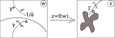
Figure 1: The correspondence between cuts in the mathematical and physical plane.

Let us fix a path $\Gamma_{m}$ from $\infty$ to $z_{m}$ lying entirely inside the domain $D(t)$ in the physical plane. It is an image of a path $\gamma^{*}_{m}$ connecting the points $\infty$ and $1/\bar{a}_{m}$ outside the unit disk: $\Gamma_{m}=f(\gamma^{*}_{m})$. Let us reflect $\gamma^{*}_{m}$ with respect to the unit circle (i.e., make the transformation $w\to 1/\bar{w}$). The reflected path, $\gamma_{m}$, connects the points $0$ and $a_{m}$ inside the unit disk. We take these $\gamma_{m}$ to be the integration paths in (44).

Take a point $w\in\gamma_{m}$ and consider two points, $w_{+}$ and $w_{-}$, which are limits to $w$ from respectively left and right sides of the branch cut $\gamma_{m}$ (oriented from $0$ to $a_{m}$). Similarly to (42), we have $f(w_{+})-f(w_{-})=\rho_{m}(w)$. The corresponding points in the physical plane, $z_{\pm}$, tend from opposite sides to the point $z=f(w^{*})\in\Gamma_{m}$, where $w^{*}=1/\bar{w}\in\gamma^{*}_{m}$ is the image of $w$ under the inversion (see Fig. 1). Since conformal maps preserve orientation, we can write $z_{\pm}=f(w^{*}_{\pm})$. However, the inversion interchanges the sides, i.e., $w^{*}_{\pm}=1/\bar{w}_{\mp}$, so $z_{\pm}=f(1/\bar{w}_{\mp})$. According to equations (10) rewritten as

$$\left\{\begin{array}[]{l}S=\bar{f}(\bar{w})\\ z=f(1/\bar{w})\,,\end{array}\right.$$ (45)

the values of the Schwarz function at $z_{\pm}$ are $S(z_{\pm})=\bar{f}(\bar{w}_{\mp})$ and the discontinuity of the Schwarz function is thus $[S(z)]=S(z_{+})-S(z_{-})=\bar{f}(\bar{w}_{-})-\bar{f}(\bar{w}_{+})=-\bar{\rho_{m}}(\bar{w})$. As singularities of $S_{+}$ and $S$ in $D(t)$ are the same, this is exactly the discontinuity of the function $S_{+}(z)$. We thus conclude that on $\gamma_{m}$ it holds

$$\rho_{m}(w)=-\bar{\mathcal{P}}_{m}(z),\quad z=\bar{f}(1/w)$$ (46)

Furthermore, since the r.h.s. is analytically extendable to the whole $\bar{D}(t)$ and the function $\bar{f}(1/w)$ sets up a conformal equivalence between $\bar{D}(t)$ and the unit disk, the $\rho_{m}(w)$ is analytically extendable from the cut $\gamma_{m}$ to the whole unit disk. Therefore, (46) actually holds everywhere in the unit disk. Plugging it into (44), we obtain the non-linear integral equation (43) for $f(w,t)$.

IV.4 The Solution Scheme

To summarize, we have the following formulas which express constants of motion through the time-dependent conformal map:

$$\begin{array}[]{l}\displaystyle{t_{1}=\frac{1}{2\pi i}\oint_{|w|=1}\frac{\bar{f}(1/w)df(w)}{f(w)}}\,,\\ \\ z_{m}\,=f(1/\bar{a}_{m}(t),t)\,.\end{array}$$ (47)

They look exactly like the corresponding formulas (32) for the logarithmic case. The main difference is that in general any explicit representation of the function $f$ is not a priori available. It is defined implicitly via the integral equation (43).

In principle, these equations supplemented by a formula for $t$ below give a solution to the problem in an implicit form, like in rational or logarithmic cases. However, the general multi-cut construction is substantially more complicated because before applying the scheme outlined in section III one has to find a solution to the integral equation (43) with required analytic properties. Clearly, such a solution depends on $a_{m}$, $u_{0}$ and $r$ as parameters: $f(w)=f(w|r,u_{0},\{a_{m}\})$. Then (47) is a system of equations to determine them through the constants of motion. The missing equation which includes $t$ can be obtained from (21) or (22). One of its forms is

$$t=r^{2}-\frac{1}{2\pi i}\sum_{m}\int_{0}^{a_{m}}\bar{\mathcal{P}}_{m}(\bar{f}(1/\zeta))\,d(\bar{f}(1/\zeta)-r/\zeta)\,,$$ (48)

Another form is

$$t=r^{2}-\sum_{l,m}\int_{0}^{a_{l}}\frac{d\zeta}{2\pi i}\int_{0}^{a_{m}}\frac{d\bar{w}}{2\pi i}\frac{\rho_{l}(\zeta)\overline{\rho_{m}(w)}}{(1-\zeta\bar{w})^{2}}$$ (49)

where $\rho_{m}(\zeta)=-\mathcal{P}_{m}(\bar{f}(1/\zeta))$. It is an analog of (35) (compare also with (29)). Meanwhile, a formula for $t_{1}$ similar to (48) also exists:

$$\bar{t}_{1}=u_{0}-\frac{1}{2\pi i}\sum_{m}\int_{0}^{a_{m}}\bar{\mathcal{P}}_{m}(\bar{f}(1/\zeta))\,d\log(\zeta\bar{f}(1/\zeta))\,,$$ (50)

which follows from (17) at $j=0$. In the case of constant densities, formulae (48) and (50) immediately give expressions (33) and (32) for $t$ and $t_{1}$ from section III.2.

V Multi-Cut Solutions with Linear Cauchy Densities

The aim of this section is to elaborate the important case of linear Cauchy densities of the Schwarz function in the physical plane. This class of solutions is characterized by the property that the second derivative of $S_{+}$ is a rational function (or, equivalently, the second derivative of $S$ is a mesomorphic function in $D(t)$). The integral equation for conformal map which is in general non-linear, becomes linear in this case. In the context of the universal Whitham hierarchy, solutions of this type were discussed in Krichever94 (section 7.2) and in KMZ05 (section 3.8). This class also includes logarithms and poles on the background of the multi-cut functions. However, the approach of the previous section is not directly applicable because the integrals become divergent.

These divergences are artificial and can be curbed for the price of introducing one more time-dependent parameter. The integral equation should be modified. We start, in subsection V.1, with a more general situation when the Cauchy densities $\mathcal{P}_{m}(z)$ are analytic everywhere in $D(t)$ except for a pole at infinity. In subsection V.2 we specify the results to the most important case of purely linear Cauchy densities. In subsection V.3 we consider, as an example, some special “finger” patterns with $\mbox{$\mathbb{Z}$}_{N}$ rotational symmetry (which are equivalent to solutions in a wedge with angle $2\pi/N$). Their asymptotic form at large $t$ is given by the known family of $\mbox{$\mathbb{Z}$}_{N}$-symmetric self-similar “fingers” described by hypergeometric solutions to the integral equation (43) (see TRHC; Benamar; BAmar; Combescot; Cummings1999; Richardson2001; MV).

V.1 Cauchy Densities with a Pole at Infinity

Let us consider the case when $\mathcal{P}_{m}(z)$ are analytic everywhere in $D(t)$ except for a simple pole at infinity. One immediately sees that neither the multi-cut ansate (41) nor the integral equation (44) can be directly applied to this case because the integrals diverge. Nevertheless, it is possible to modify these formulas in such a way that the divergences disappear. To this end, consider a modified multi-cut ansate:

$$S_{+}(z)=t_{1}+2t_{2}z+\sum_{m}\int_{\infty,\Gamma_{m}}^{z_{m}}\frac{z^{2}\mathcal{P}_{m}(\tau)}{\tau^{2}(\tau-z)}\,\frac{d\tau}{2\pi i}\,,$$ (51)

where $t_{1}$ and $t_{2}$ are arbitrary complex constants (the first and the second harmonic moments) and we adopt the same conventions about the cuts $\Gamma_{m}$ as before. A single-valued branch of this function is fixed by the conditions $S_{+}(0)=t_{1}$, $S_{+}^{\prime}(0)=2t_{2}$. Let us plug it into the integral equation (II) with $d=1$. A simple calculation similar to the one done in section IV.3 yields the integral equation

$$f(w)=rw+u_{0}+\frac{u_{1}}{w}-\sum_{m}\int_{0}^{a_{m}}\frac{\zeta\bar{\mathcal{P}}_{m}(\bar{f}(1/\zeta))}{w(\zeta-w)}\,\frac{d\zeta}{2\pi i}$$ (52)

The general scheme of solution remains the same, with the only difference that now we have one more time-dependent parameter (the coefficient $u_{1}$). Accordingly, we need an extra equation connecting it with integrals of motion. The necessary equations, which generalize (33) and (32), can be obtained from (17), (18). They are:

$$2\bar{t}_{2}=\frac{u_{1}}{r}+\frac{1}{2\pi i}\sum_{m}\int_{0}^{a_{m}}\bar{\mathcal{P}}_{m}(\bar{f}(1/\zeta))d\left(\frac{1}{\bar{f}(1/\zeta)}-\frac{\zeta}{r}\right)$$

$$\bar{t}_{1}=u_{0}-\frac{u_{1}\bar{u}_{0}}{r}-$$

$$\frac{1}{2\pi i}\sum_{m}\int_{0}^{a_{m}}\bar{\mathcal{P}}_{m}(\bar{f}(1/\zeta))d\left(\log(\zeta\bar{f}(1/\zeta))-\frac{\bar{u}_{0}\zeta}{r}\right)$$

$$t=r^{2}-|u_{1}|^{2}-$$

$$\frac{1}{2\pi i}\sum_{m}\int_{0}^{a_{m}}\bar{\mathcal{P}}_{m}(\bar{f}(1/\zeta))\,d\left(\bar{f}(1/\zeta)-\frac{r}{\zeta}-\bar{u}_{1}\zeta\right).$$ (53)

Let us briefly comment on a more general case of Cauchy densities with a higher pole at infinity (and analytic everywhere else in $D(t)$). It should be already clear how to proceed. If the leading term of $\mathcal{P}_{m}(z)$ as $z\to\infty$ is $z^{d}$, then one should extract from $S_{+}(z)$ a polynomial $\sum_{k=1}^{d+1}kt_{k}z^{k-1}$ of degree $d$ and represent the remaining part (which is of order $O(z^{d+1})$ as $z\to 0$) as integrals along the cuts. Plugging this ansate into (II), one obtains an integral equation for the conformal map containing a Laurels polynomial $rw+\sum_{j=0}^{d}u_{j}w^{-j}$ in the r.h.s. So, apart from positions of branch points, there are $d+2$ time-dependent parameters $r,u_{0},\ldots,u_{d}$ which are to be connected with integrals of motion by formulae similar to (V.1).

V.2 Linear Cauchy Densities

The case of linear homogeneous Cauchy densities is especially important. Set

$$\mathcal{P}_{m}(z)=2\pi i\,c_{m}z\,,$$ (54)

where $c_{m}$ are arbitrary complex constants. The explicit form of the function $S_{+}$ is:

$$S_{+}(z)=t_{1}+2t_{2}z+z\sum_{m}c_{m}\log\left(1-\frac{z}{z_{m}}\right)\,,$$ (55)

It is clear that the integral equation (52) becomes linear:

$$f(w)=rw+u_{0}+\frac{u_{1}}{w}+\sum_{m}\bar{c}_{m}\int_{0}^{a_{m}}\frac{\zeta\bar{f}(1/\zeta)d\zeta}{w\,(\zeta-w)}\,.$$ (56)

Formulae (12) read:

$$2\bar{t}_{2}=\frac{u_{1}}{r}-\sum_{m}\bar{c}_{m}\int_{0}^{a_{m}}\bar{f}(1/\zeta)\,d\left(\frac{1}{\bar{f}(1/\zeta)}-\frac{\zeta}{r}\right)$$

$$\bar{t}_{1}=u_{0}-\frac{u_{1}\bar{u}_{0}}{r}+$$

$$\sum_{m}\bar{c}_{m}\int_{0}^{a_{m}}\bar{f}(1/\zeta)\,d\left(\log(\zeta\bar{f}(1/\zeta))-\frac{\bar{u}_{0}\zeta}{r}\right)$$

$$t=r^{2}-|u_{1}|^{2}+$$

$$\sum_{m}\bar{c}_{m}\int_{0}^{a_{m}}\bar{f}(1/\zeta)\,d\left(\bar{f}(1/\zeta)-\frac{r}{\zeta}-\bar{u}_{1}\zeta\right)$$ (57)

After some simple transformations, they can be brought to the form

$$2\bar{t}_{2}=\frac{u_{1}}{r}+$$

$$\sum_{m}\bar{c}_{m}\left[\log\left(\frac{a_{m}\bar{z}_{m}}{r}\right)+\frac{1}{r}\int_{0}^{a_{m}}\left(\bar{f}(1/\zeta)-r/\zeta\right)d\zeta\right]$$ (58)

$$\bar{t}_{1}=u_{0}-2\bar{u}_{0}\bar{t}_{2}+$$

$$\sum_{m}\bar{c}_{m}\left[\bar{z}_{m}+\bar{u}_{0}\log\left(\frac{a_{m}\bar{z}_{m}}{r}\right)-\bar{u}_{0}-\frac{r}{a_{m}}+\right.$$

$$\left.\int_{0}^{a_{m}}\left(\bar{f}(1/\zeta)-r/\zeta-\bar{u}_{0}\right)\frac{d\zeta}{\zeta}\right]$$ (59)

$$t=r^{2}-2r\bar{u}_{1}\bar{t}_{2}+$$

$$\sum_{m}\bar{c}_{m}\left[\frac{\bar{z}_{m}^{2}}{2}+r\bar{u}_{1}\log\left(\frac{a_{m}\bar{z}_{m}}{r}\right)-\frac{\bar{u}_{0}^{2}}{2}-r\bar{u}_{1}-\frac{r^{2}}{2a_{m}^{2}}-\right.$$

$$\left.\frac{r\bar{u}_{0}}{a_{m}}+r\int_{0}^{a_{m}}\left(\bar{f}(1/\zeta)-r/\zeta-\bar{u}_{0}-\bar{u}_{1}\zeta\right)\frac{d\zeta}{\zeta^{2}}\right]$$ (60)

Let us specify the scheme of solution to the case of linear densities. Suppose one is able to find a solution to the linear integral equation (56) depending on the parameters $a_{m}$, $u_{0}$, $u_{1}$ and $r$: $f(w)=f(w|r,u_{0},u_{1},\{a_{m}\})$ (with fixed $c_{m}$). Then, since $f(1/\bar{a}_{m})=z_{m}$ are constants of motion, we get a system of equations for $a_{m}$, $u_{0}$, $u_{1}$ and $r$ which becomes closed after adding equations (58), (59), (60). This system determines the parameters as implicit functions of $t$.

We conclude the subsection with a remark that the solutions of the linear integral equation (56) for the conformal map $f(w,t)$, which correspond to linear Cauchy density of the Schwarz function defined by (55), deserve a special name in view of their importance. So, in what follows we will refer to them as to hyper-logarithmic solutions, since they contain logarithmic solutions (31) and the Gauss hyper-geometric function (see (70) below) as particular cases.

V.3 Example: $\mbox{$\mathbb{Z}$}_{N}$-Symmetric Solutions with $N$ Radial Cuts

In this subsection we consider perhaps the simplest non-trivial application of the linear integral equation derived above: growing patterns with $\mbox{$\mathbb{Z}$}_{N}$ rotational symmetry whose Schwarz function has exactly $N$ radial branch cuts in $D(t)$ with linear Cauchy densities.

Let $\omega=e^{2\pi i/N}$ be the primitive root of unity of degree $N$. The $\mbox{$\mathbb{Z}$}_{N}$-symmetry implies $S(\omega z)=\omega^{-1}S(z)$. Moreover, this relation holds for both $+$ and $-$ parts of the Schwarz function separately: $S_{\pm}(\omega z)=\omega^{-1}S_{\pm}(z)$. This prompts us to choose the constants of motion in the form

$$\!\!\!c_{m}=c\omega^{-2m+2},\quad z_{m}=\lambda\omega^{m-1},\quad m=1,2,\ldots,N,$$ (61)

with real positive constants $c$ and $\lambda$, so the function $S_{+}$ is

$$S_{+}(z)=cz\sum_{m=0}^{N-1}\omega^{-2m}\log\left(1-\frac{z\omega^{-m+1}}{\lambda}\right)=$$

$$-\frac{cz^{N-1}}{(1-\frac{2}{N})\lambda^{N-2}}\!\phantom{a}_{2}F_{1}\left(\begin{array}[]{c}1,\,\,1\!-\!\frac{2}{N}\\ 2-\frac{2}{N}\end{array},(z/\lambda)^{N}\right),$$ (64)

where $\!\!\!\phantom{a}{}_{2}F_{1}$ is the Gauss hypergeometric function.

For the conformal map the $\mbox{$\mathbb{Z}$}_{N}$-symmetry means $f(\omega^{k}w)=\omega^{k}f(w)$, so the expansion of the function $f(w)/w$ goes in powers of $w^{-N}$:

$$f(w)/(rw)=1+\sum_{k\geq 1}f_{k}w^{-kN}$$

where $f_{k}\equiv u_{kN}/r$. The reality of $c$ and $\lambda$ in (V.3) implies that the coefficients $f_{k}$ are real, i.e., $\bar{f}(w)=f(w)$. In what follows we assume that $N\geq 3$, so the coefficients $u_{0}$ and $u_{1}$ in the expansion of $f(w)$ (2) are always identically zero.

We use the integral equation (56). Substituting our data, we get

$$f(w)=rw+c\sum_{m=0}^{N-1}\omega^{2m}\int_{0}^{a\omega^{m}}\frac{\zeta f(1/\zeta)d\zeta}{w(\zeta-w)}$$ (65)

where $a$ is a point between $0$ and $1$ such that $f(1/a)=\lambda$. Choosing the integration paths to be straight lines from $0$ to $a\omega^{m}$ and using the $\mbox{$\mathbb{Z}$}_{N}$-symmetry, we arrive at the equation

$$f(w)=rw+cN\int_{1/a}^{\infty}\frac{wf(x)\,dx}{1-w^{N}x^{N}},$$ (66)

where $c$ is a constant and $r$, $a$ depend on time. Let $f(w)=f(w|r,a)$ be a solution to this integral equation with parameters $r,a$, then three parameters $r$, $a$ and $t$ are connected by two equations which determine $r$, $a$ as implicit functions of $t$. The first of these equations is obtained from the fact that $\lambda=f(1/a(t),t)$ is a constant of motion by substituting $w=1/a$ into (66):

$$r=\lambda a-cN\int_{1/a}^{\infty}\frac{f(x|r,a)\,dx}{1-x^{N}a^{-N}}\,,$$ (67)

the second is one or another version of the formula for $t$ in terms of $f(w)$.

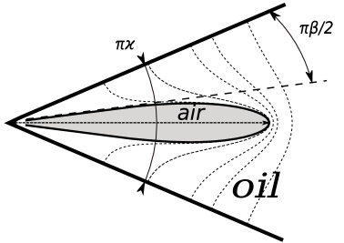
Figure 2: Laplacian Growth in wedge geometry. Air is pushed into oil trough the corner of the wedge. $\beta$ is the fjord angle.

We have obtained a one-parametric family of exact solutions to the LG describing growth of $N$ symmetric air fingers or, what is mathematically the same, growth of an air finger in the wedge with interior angle $2\pi/N$ (Fig. 2). It is not clear at the moment whether the conformal map $f(w)$ is available in a closed analytic form. However, the solution can be analyzed numerically (see appendix A).

What is the meaning of the parameter $c$? To answer this question, consider the limit $t\to\infty$, wherein, as one can easily show, $a\to 1$. Then equation (66) becomes identical to the linear integral equation describing self-similar growth of $\mbox{$\mathbb{Z}$}_{N}$-symmetric fingers (or fingers in the wedge with interior angle $2\pi/N$):

$$f(w)=rw+\frac{N\sin\pi\beta}{\pi}\int_{1}^{\infty}\frac{wf(x)\,dx}{1-w^{N}x^{N}}$$ (68)

with the “boundary condition” $f(1)=0$. As shown in our earlier paper AMZ, $\beta$ is the interior angle of the oil fjord between two neighboring air fingers. Since $c$ in (66) is a constant of motion, we conclude that setting

$$c=\frac{\sin\,\pi\beta}{\pi}$$ (69)

we can interpret $\beta$ as the asymptotic fjord angle.

Meanwhile, an analytic solution of (68) in terms of the Gauss hypergeometric function is available:

$$f(w)=rw(1-w^{-N})^{\beta}\phantom{a}_{2}F_{1}\left(\begin{array}[]{c}\beta,\,\,\beta\!-\!\kappa\\ 1-\kappa\end{array},w^{-N}\right).$$ (70)

where

$$\kappa=\frac{2}{N}\,.$$

For more details, see AMZ, where the self-similar case was studied in detail.

The integral equation (66) is equivalent to an infinite system of linear equations for the coefficients $f_{k}$. To represent it in this form, let us introduce a function $F$ via

$$f(w)=rwF(w^{-N})\,,\quad F(w)=\sum_{k=0}^{\infty}f_{k}w^{k}\,,\quad f_{0}=1\,,$$

then the integral equation (66) becomes

$$F(w)=1+c\int_{0}^{\alpha}\frac{x^{-\kappa}F(x)\,dx}{x-w^{-1}}\,,$$ (71)

where $\alpha=a^{N}$. Substituting the Taylor expansion of $F$ and comparing the coefficients, we get

$$f_{j}=-c\sum_{k=0}^{\infty}\frac{\alpha^{j+k-\kappa}}{j+k-\kappa}\,f_{k}\,,\quad j\geq 1\,.$$ (72)

(However, because the r.h.s. contains $f_{0}=1$, this is not an eigenvalue equation but rather an inhomogeneous system of linear equations.) It is also useful to note the formula for $t$,

$$t=r^{2}+\frac{1}{2}Nc\lambda^{2}+cr^{2}\sum_{n\geq 0}\frac{\alpha^{n-\kappa}f_{n}}{n-\kappa}\,,$$ (73)

which follows from (60).

VI Discussion and Conclusion

In conclusion, let us briefly comment on the following three major points of this work:

• The inverse potential problem integral equation, (15) (or (20)),

• The equations for multi-cut solutions, (41) and (43),

• The equations for hyper-logarithmic solutions, (55) and (56).

The inverse potential problem equation (15): The formulation of the LG problem as a linear growth of a domain area with conserved harmonic moments requires to solve the inverse potential problem, namely to find the conformal map $f(w)$ from the function $S_{+}(z)=\sum_{k=1}^{\infty}kt_{k}z^{k-1}$, whose Taylor coefficients are conserved harmonic moments of the growing domain and from the area/time $t$. While it is straightforward to obtain $S_{+}(z)$ and $t$ from $f(w)$ (the direct potential problem), it is a well-known challenge to do it the other way around (the inverse potential problem) Gust. The reformulation of the inverse potential problem as the nonlinear integral equation (15) (or (20)) for the function $f(w)$, assuming that $S_{+}(z)$ is known, appears to be extremely useful. In particular, it allows us to obtain some important classes of solutions to the LG problem with prescribed integrals of motion (harmonic moments), including those with arbitrary branch cuts as well as those with pole singularities. This integral equation is also expected to be of significant help in a future work on LG and related problems of interface dynamics.

The equation for multi-cut solutions, (43): A mathematical motivation for this work was a strong feeling that rational and logarithmic conformal maps do not exhaust the list of exact solutions of LG at zero surface tension. A physical motivation came from a long standing need to describe most general moving interfaces in Hele-Shaw experiments with negligible surface tension. As was already said in section IV.1, while finite linear combinations of logarithms can describe interface dynamics without finite time singularities, they fail to describe an interface with non-parallel fjords walls. This motivated us to look for a more general family of solutions to the LG equation (3). We expect that the multi-cut solutions presented in this paper do explain the experiments Couder; HLS-DLA; Leif where formation and development of oil fjords with non-parallel and/or non-straight walls was observed.

Two special kinds of branch points and cut singularities were already considered in earlier works on Laplacian growth. Fractional time-independent branch points appeared in studies of self-similar singular interfaces BAmar; Tu; AMZ, while logarithmic branch cuts with constant Cauchy densities appeared in H86; BP86; MS94; SM94; SM98. We have shown that all of them are just various special cases and limits of the presented general construction. In the light of our approach, it also becomes clear why the pole and logarithmic solutions are special: the Cauchy densities are particularly simple in these cases, so the integral equation can be easily solved. It also shows a road to obtain new families of exact solutions.

The equation for hyper-logarithmic solutions, (56): The mathematical significance of the hyper-logarithmic solutions is that they correspond to the linear integral equation (56), which ought to be much more accessible to analytic treatment than the general nonlinear equation (43) for multi-cut solutions. The physical importance lies in the belief that the hyper-logarithmic solutions describe fjords with a constant opening angle, in agreement with viscous fingering experiments Leif. The interface dynamics simulated in a wedge, shown on Figure 3, seems to confirm this belief, if to consider fjords central lines as walls of virtual wedges in accordance with Couder. A thorough geometric analysis of the corresponding interface dynamics based on the integral equation (56) will be published elsewhere.

VII Acknowledgement

Ar.A is grateful to Welch Foundation for the partial support. His work was also partially supported by NF PhD-0757992 grant. All authors gratefully acknowledge a significant help from the project 20070483ER at the LDRD programs of LANL: the work of M.M-W. on this problem was fully supported by this project, while two other authors were partially supported by the same grant during their visits to LANL in 2008. The work of A.Z. was also partially supported by grants RFBR 08-02-00287, RFBR-06-01-92054-$\mbox{CE}_{a}$, Nsh-3035.2008.2 and NWO 047.017.015. A.Z. thanks the Galileo Galilei Institute for Theoretical Physics for the hospitality and the INFIN for partial support during the completion of this work.

Appendix A Numerical solution of equation (66)

Equation (66) with $c$ given by (69) can be rewritten in the following way:

$$\!\!\!\!f(w,t)\!=\!r(t)w\!-\!\frac{N\sin\pi\beta}{\pi}w\oint_{|\zeta|=1}\!\!\!\!\!\!\!\!\!\frac{f(\zeta,t)\log(1-a(t)\zeta)}{1-w^{N}\zeta^{N}}\frac{d\zeta}{2\pi i},$$

$$\!\!\!\!f(1/a(t),t)=\lambda,$$ (74)

We are looking for a solution consistent with the $\mbox{$\mathbb{Z}$}_{N}$-symmetry:

$$f(w,t)=r(t)w+\sum_{k=1}^{\infty}f_{k}(t)w^{-Nk+1}$$ (75)

Equation (A) then takes the form

$$f_{n}(t)=-r(t)\frac{\sin\pi\beta}{\pi}\frac{\alpha^{n-\kappa}(t)}{n-\kappa}-$$

$$\frac{N\sin\pi\beta}{\pi}\sum_{k=1}^{\infty}f_{k}(t)\frac{\alpha^{n+k-\kappa}(t)}{n+k-\kappa}.$$ (76)

where $\kappa=2/N$, $\alpha=a^{N}$. Using the relation $\lambda=f(1/a(t),t)$ and re-denoting $f_{k}(\alpha)\equiv f_{k}(t(\alpha))$, $r(\alpha)\equiv r(t(\alpha))$, we get

$$r(\alpha)=\alpha^{\kappa/2}\lambda-\sum_{k=1}^{\infty}f_{k}(\alpha)\alpha^{k},$$ (77)

and

$$\sum_{k=1}^{\infty}f_{k}(\alpha)\frac{k\alpha^{n+k}}{n+k-\kappa}\!\!-\!\!\frac{\pi(n-\kappa)}{\sin\pi\beta}\alpha^{\kappa}f_{n}(\alpha)=\lambda\alpha^{n+\kappa/2}$$ (78)

This equation is easily solved numerically for any given $\alpha$ . The conformal radius $r$ and the time are then found from (77) and (22) (or (73)) respectively. The solution is shown in figure 3.

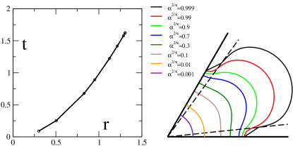
Figure 3: (color online) The results of the numerical solution of the equation (66) for $N=6$, $\beta=0.4/N$. The left panel shows the dependence of the area $t$ on the conformal radius $r$, the right panel shows the growing finger at different times.

References

References

-
(1)
K.A.Gillow and S.D.Howison,
A bibliography of free and moving boundary problems for Hele-Shaw and Stokes flow.
http://www.maths.ox.ac.uk/
howison/Hele-Shaw/ . “bibitem–KMWZ˝ I. Krichever, M. Mineev-Weinstein, P. Wiegmann, and A. Zabrodin, Physica D –“bf 198˝, 1 (2004), arXiv:nlin.SI/0311005. “bibitem–Gust˝ B. Gustafsson and A. Vasil’ev, –“it Conformal and Potential Analysis in Hele-Shaw Cells (Advances in Mathematical Fluid Mechanics)˝, (Birkh“”–a˝user, Basel, 2006), 1st ed., ISBN 3764377038. “bibitem–Richardson˝ S. Richardson, J. Fluid Mech., –“bf 56˝, 609-618 (1972). “bibitem–MWZ˝ M. Mineev-Weinstein, P. Wiegmann, A. Zabrodin, Phys. Rev. Lett., –“bf 84˝, 5106–5109, (2000). “bibitem–KKMWZ˝ I.Kostov, I.Krichever, M.Mineev-Weinstein, P.Wiegmann, and A.Zabrodin, in –“it Random Matrix Models and Their Applications˝, ed. by P.Bleher and A.Its, (Cambridge: Cambridge Academic Press, 2001), vol.40 of –“it Random Matrices and Their Applications (MSRI publications)˝, pp. 285-299. “bibitem–Kuf˝ P. Kufarev, Doklady Akademii Nauk SSSR, –“bf 60˝, 1333 (1948). “bibitem–SB84˝ B. Shraiman, and D. Bensimon, Phys. Rev. A, –“bf 30˝, 2840 (1984). “bibitem–M90˝ M. Mineev-Weinstein, Physica D, –“bf 43˝, 288 (1990). “bibitem–H86˝ S. D. Howison, Journal of Fluid Mechanics, –“bf 167˝, 439 (1986). “bibitem–BP86˝ D. Bensimon, and P. Pelc“’e, Phys. Rev. A, –“bf 33˝, 4477 (1986). “bibitem–MS94˝ M. B. Mineev-Weinstein and S. P. Dawson, Phys. Rev. E –“bf 50˝,R24 (1994). “bibitem–SM94˝ S. P. Dawson and M. B. Mineev-Weinstein, Physica D, –“bf 83˝, 383(1994). “bibitem–BAmar˝ M. Ben Amar, Phys. Rev. A, –“bf 44˝, 3673 (1991). “bibitem–Tu˝ Y. Tu, Phys. Rev. A, –“bf 44˝, 1203 (1991). “bibitem–AMZ˝ Ar. Abanov, M. Mineev-Weinstein, and A. Zabrodin, Physica D, –“bf 235˝, 62 (2007). “bibitem–Hele-Shaw1898˝ H. S. Hele––˝Shaw, Nature, –“bf 58˝, 1489 (1898). “bibitem–RMP86˝ D. Bensimon, L. P. Kadanoff, S. Liang, B. I. Shraiman, and C. Tang, Rev. Mod. Phys., –“bf 58˝, 977 (1986). “bibitem–Galin˝ L. Galin, Dokl. Akad. Nauk. S.S.S.R., –“bf 47˝, 246 (1945). “bibitem–PK45˝ P. Polubarinova–Kochina, Dokl. Akad. Nauk. S.S.S.R., –“bf 47˝, 254 (1945). “bibitem–H92˝ S. D. Howison, European Journal of Applied Mathematics, –“bf 3˝, 209 (1992). “bibitem–Davis˝ P. J. Davis, –“it The Schwarz function and its applications.˝ (The Carus Math. Monographs, No. 17, The Math. Association of America, Buffalo, N.Y., 1974.) “bibitem–KMZ05˝ I. Krichever, A. Marshakov, and A. Zabrodin, Commun. Math. Phys., –“bf 259˝, 1 (2005). “bibitem–Krichever94˝ I. Krichever, Commun. Pure Appl. Math., –“bf 437˝, 437 (1994). “bibitem–SM98˝ S. P. Dawson and M. Mineev-Weinstein, Phys. Rev. E, –“bf 57˝, 3063 (1998). “bibitem–Paterson˝ L. Paterson, Journal of Fluid Mechanics, –“bf 113˝, 513 (1981). “bibitem–Sander˝ L. M. Sander and P. Ramanlal and E. Ben Jacob, Phys. Rev. A, –“bf 32˝, R3160 (1985). “bibitem–Couder˝ E. Lageunesse and Y. Couder, Journal of Fluid Mechanics, –“bf 419˝, 125 (2000). “bibitem–Leif˝ L. Ristroph, M. Thrasher, M. Mineev-Weinstein and H. L. Swinney, Physical Review E, (RC), –“bf 74˝, 015201-1 (2006). “bibitem–TRHC˝ H. Thome, M. Rabaud, V. Hakim, and Y. Couder, Physics of Fluids A: Fluid Dynamics, –“bf 1˝, 224 (1989). “bibitem–Benamar˝ M. Ben Amar, Phys. Rev. A, –“bf 43˝, 5724 (1991). “bibitem–Combescot˝ R. Combescot, Phys. Rev. A, –“bf 45˝, 873 (1992). “bibitem–Cummings1999˝ L. Cummings, Euro. J. Appl. Math., –“bf 10˝, 547 (1999). “bibitem–Richardson2001˝ S. Richardson, Euro. J. Appl. Math., –“bf 12˝, 665 (2001). “bibitem–MV˝ I. Markina and A. Vasil’ev, Euro. J. Appl. Math., –“bf 15˝, 781 (2004). “bibitem–HLS-DLA˝ O. Praud and H. L. Swinney, Phys. Rev. E, –“bf 72˝, 011406 2005). “end–thebibliography˝ “end–document˝