Secret Sharing over Fast-Fading MIMO Wiretap Channels

Abstract

Secret sharing over the fast-fading MIMO wiretap channel is considered. A source and a destination try to share secret information over a fast-fading MIMO channel in the presence of an eavesdropper who also makes channel observations that are different from but correlated to those made by the destination. An interactive, authenticated public channel with unlimited capacity is available to the source and destination for the secret sharing process. This situation is a special case of the “channel model with wiretapper” considered by Ahlswede and Csiszár. An extension of their result to continuous channel alphabets is employed to evaluate the key capacity of the fast-fading MIMO wiretap channel. The effects of spatial dimensionality provided by the use of multiple antennas at the source, destination, and eavesdropper are then investigated.

I Introduction

The wiretap channel considered in the seminal paper [1] is the first example that demonstrates the possibility of secure communications at the physical layer. It is shown in [1] that a source can transmit a message at a positive (secrecy) rate to a destination in such a way that an eavesdropper only gathers information at a negligible rate, when the source-to-eavesdropper channel is a degraded version of the source-to-destination channel. A similar result for the Gaussian wiretap channel is provided in [2]. The work in [3] further removes the degraded wiretap channel restriction showing that positive secrecy capacity is possible if the destination channel is “more capable” (“less noisy” for a full extension of the rate region in [1]) than the eavesdropper’s channel. Recently, there has been a flurry of interest in extending these early results to more sophisticated channel models, including fading wiretap channels, multi-input multi-output (MIMO) wiretap channels, multiple-access wiretap channels, broadcast wiretap channels, relay wiretap channels, etc. We do not attempt to provide a comprehensive summary of all recent developments, and highlight only results that are most relevant to the present work. We refer interested readers to the introduction and reference list of [4] for a concise and extensive overview of recent works.

When the destination and eavesdropper channels experience independent fading, the strict requirement of having a more capable destination channel for positive secrecy capacity can be loosened. This is due to the simple observation that the destination channel may be more capable than the eavesdropper’s channel under some fading realizations, even if the destination is not more capable than the eavesdropper on average. Hence, if the channel state information (CSI) of both the destination and eavesdropper channels is available at the source, it is shown in [4, 5] that a positive secrecy capacity can be achieved by means of appropriate power control at the source. The key idea is to opportunistically transmit only during those fading realizations for which the destination channel is more capable [6]. For block-ergodic fading, it is also shown in [5] (see also [7]) that a positive secrecy capacity can be achieved with a variable-rate transmission scheme without any eavesdropper CSI available at the source.

When the source, destination, and eavesdropper have multiple antennas, the resulting channel is known as a MIMO wiretap channel (see [8, 9, 10, 11, 12]), which may also have positive secrecy capacity. Since the MIMO wiretap channel is not degraded, the characterization of its secrecy capacity is not straightforward. For instance, the secrecy capacity of the MIMO wiretap channel is characterized in [9] as the saddle point of a minimax problem, while an alternative characterization based on a recent result for multi-antenna broadcast channels is provided in [11]. Interestingly all characterizations point to the fact that the capacity achieving scheme is one that transmits only in the directions in which the destination channel is more capable than the eavesdropper’s channel. Obviously, this is only possible when the destination and eavesdropper CSI is available at the source. It is shown in [9] that if the individual channels from antennas to antennas suffer from independent Rayleigh fading, and the respective ratios of the numbers of source and destination antennas to that of eavesdropper antennas are larger than certain fixed values, then the secrecy capacity is positive with probability one when the numbers of source, destination, and eavesdropper antennas become very large.

As discussed above, the availability of destination (and eavesdropper) CSI at the source is an implicit requirement for positive secrecy capacity in the fading and MIMO wiretap channels. Thus, an authenticated feedback channel is needed to send the CSI from the destination back to the source. In [5, 7], this feedback channel is assumed to be public, and hence the destination CSI is also available to the eavesdropper. In addition, it is assumed that the eavesdropper knows its own CSI. With the availability of a feedback channel, if the objective of having the source send secret information to the destination is relaxed to distilling a secret key shared between the source and destination, it is shown in [13] that a positive key rate is achievable when the destination and eavesdropper channels are two conditionally independent (given the source input symbols) memoryless binary channels, even if the destination channel is not more capable than the eavesdropper’s channel. This notion of secret sharing is formalized in [14] based on the concept of common randomness between the source and destination. Assuming the availability of an interactive, authenticated public channel with unlimited capacity between the source and destination, [14] suggests two different system models, called the “source model with wiretapper” (SW) and the “channel model with wiretapper” (CW). The CW model is the similar to the (discrete memoryless) wiretap channel model that we have discussed before. The SW model differs in that the random symbols observed at the source, destination, and eavesdropper are realizations of a discrete memoryless source with multiple components. Both SW and CW models have been extended to the case of secret sharing among multiple terminals, with the possibility of some terminals acting as helpers [15, 16, 17]. Key capacities have been obtained for the two special cases in which the eavesdropper’s channel is a degraded version of the destination channel and in which the destination and eavesdropper channels are conditionally independent [14, 13]. Similar results have been derived for multi-terminal secret sharing [16, 17], with the two special cases above subsumed by the more general condition that the terminal symbols form a Markov chain on a tree. Authentication of the public channel can be achieved by the use of an initial short key and then a small portion of the subsequent shared secret message [18]. A detailed study of secret sharing over an unauthenticated public channel is given in [19, 20, 21].

Other approaches to employ feedback have also been recently considered [22, 24, 23]. In particular, it is shown in [22] that positive secrecy capacity can be achieved for the modulo-additive discrete memoryless wiretap channel and the modulo-$\Lambda$ channel if the destination is allowed to send signals back to the source over the same wiretap channel and both terminals can operate in full-duplex manner. In fact, for the former channel, the secrecy capacity is the same as the capacity of such a channel in the absence of the eavesdropper.

In this paper, we consider secret sharing over a fast-fading MIMO wiretap channel. Thus, we are interested in the CW model of [14] with memoryless conditionally independent destination and eavesdropper channels and continuous channel alphabets. We provide an extension of the key capacity result in [14] for this case to include continuous channel alphabets (Theorem II.1). Using this result, we obtain the key capacity of the fast-fading MIMO wiretap channel (Section III). Our result indicates that the key capacity is always positive, no matter how large the channel gain of the eavesdropper’s channel is; in addition this holds even if the destination and eavesdropper CSI is available at the destination and eavesdropper, respectively. Of course, the availability of the public channel implies that the destination CSI could be fed back to the source. However, due to the restrictions imposed on the secret-sharing strategies (see Section II), only causal feedback is allowed, and thus any destination CSI available at source is “outdated”. This does not turn out to be a problem since, unlike the approaches mentioned above, the source does not use the CSI to avoid sending secret information when the destination is not more capable than the eavesdropper’s channel. As a matter of fact, the fading process of the destination channel provides a significant part of the common randomness from which the source and the destination distill a secret key. This fact is readily obtained from the alternative achievability proof given in Section IV. We note that [25, 26] consider the problem key generation from common randomness over wiretap channels and exploit a Wyner-Ziv coding scheme to limit the amount of information conveyed from the source to the destination via the wiretap channel. Unlike these previous works, we only employ Wyner-Ziv coding to quantize the destination channel outputs. Our code construction still relies on a public channel with unlimited capacity to achieve the key capacity.

Finally, we also investigate the limiting value of the key capacity under three asymptotic scenarios. In the first scenario, the transmission power of the source becomes asymptotically high (Corollary III.1). In the second scenario, the destination and eavesdropper have a large number of antennas (Corollary III.2). In the third scenario, the gain advantage of the eavesdropper’s channel becomes asymptotically large (Corollary III.3). These three scenarios reveal two different effects of spatial dimensionality upon key capacity. In the first scenario, we show that the key capacity levels off as the power increases if the eavesdropper has no fewer antennas than the source. On the other hand, when the source has more antennas, the key capacity can increase without bound with the source power. In the second scenario, we show that the spatial dimensionality advantage that the eavesdropper has over the destination has exactly the same effect as the channel gain advantage of the eavesdropper. In the third scenario, we show that the limiting key capacity is positive only if the eavesdropper has fewer antennas than the source. The results in these scenarios confirm that spatial dimensionality can be used to combat the eavesdropper’s gain advantage, which was already observed for the MIMO wiretap channel. Perhaps more surprisingly, this is achieved with neither the source nor destination needing any eavesdropper CSI.

II Secret Sharing and Key Capacity

We consider the CW model of [14], and we recall its characteristics for completeness. We consider three terminals, namely a source, a destination, and an eavesdropper. The source sends symbols from an alphabet $\mathcal{X}$. The destination and eavesdropper observe symbols belonging to alphabets $\mathcal{Y}$ and $\mathcal{Z}$, respectively. Unlike in [14], $\mathcal{X}$, $\mathcal{Y}$, and $\mathcal{Z}$ need not be discrete. In fact, in Section III we will assume they are multi-dimensional vector spaces over the complex field. The channel from the source to the destination and eavesdropper is assumed memoryless. A generic symbol sent by the source is denoted by $X$ and the corresponding symbols observed by the destination and eavesdropper are denoted by $Y$ and $Z$, respectively. For notational convenience (and without loss of generality), we assume that $(X,Y,Z)$ are jointly continuous, and the channel is specified by the conditional probability density function (pdf) $p_{Y,Z|X}(y,z|x)$. In addition, we restrict ourselves to cases in which $Y$ and $Z$ are conditionally independent given $X$, i.e., $p_{Y,Z|X}(y,z|x)=p_{Y|X}(y|x)p_{Z|X}(z|x)$, which is a reasonable model for symbols broadcasted in a wireless medium. Hereafter, we drop the subscripts in pdfs whenever the concerned symbols are well specified by the arguments of the pdfs. We assume that an interactive, authenticated public channel with unlimited capacity is also available for communicatin between the source and destination. Here, interactive means that the channel is two-way and can be used multiple times, unlimited capacity means that it is noiseless and has infinite capacity, and public and authenticated mean that the eavesdropper can perfectly observe all communications over this channel but cannot tamper with the messages transmitted.

We consider the class of permissible secret-sharing strategies suggested in [14]. Consider $k$ time instants labeled by $1,2,\ldots,k$, respectively. The $(X,Y,Z)$ channel is used $n$ times during these $k$ time instants at $i_{1}<i_{2}<\cdots<i_{n}$. Set $i_{n+1}=k$. The public channel is used for the other ($k-n$) time instants. Before the secret-sharing process starts, the source and destination generate, respectively, independent random variable $M_{X}$ and $M_{Y}$. To simplify the notation, let $a^{i}$ represent a sequence of messages/symbols $a_{1},a_{2},\ldots,a_{i}$. Then a permissible strategy proceeds as follows:

• At time instant $0<i<i_{1}$, the source sends message $\Phi_{i}=\Phi_{i}(M_{X},\Psi^{i-1})$ to the destination, and the destination sends message $\Psi_{i}=\Psi_{i}(M_{Y},\Phi^{i-1})$ to the source. Both transmissions are carried over the public channel.

• At time instant $i=i_{j}$ for $j=1,2,\ldots,n$, the source sends the symbol $X_{j}=X_{j}(M_{X},\Psi^{i_{j}-1})$ to the $(X,Y,Z)$ channel. The destination and eavesdropper observe the corresponding symbols $Y_{j}$ and $Z_{j}$. There is no message exchange via the public channel, i.e., $\Phi_{i}$ and $\Psi_{i}$ are both null.

• At time instant $i_{j}<i<i_{j+1}$ for $j=1,2,\ldots,n$, the source sends message $\Phi_{i}=\Phi_{i}(M_{X},\Psi^{i-1})$ to the destination, and the destination sends message $\Psi_{i}=\Psi_{i}(M_{Y},Y^{j},\Phi^{i-1})$ to the source. Both transmissions are carried over the public channel.

At the end of the $k$ time instants, the source generates its secret key $K=K(M_{X},\Psi^{k})$, and the destination generates its secret key $L=L(M_{Y},Y^{n},\Phi^{k})$, where $K$ and $L$ takes values from the same finite set $\mathcal{K}$.

According to [14], $R$ is an achievable key rate through the channel $(X,Y,Z)$ if for every $\varepsilon>0$, there exists a permissible secret-sharing strategy of the form described above such that

1. $\Pr\{K\neq L\}<\varepsilon$,

2. $\frac{1}{n}I(K;Z^{n},\Phi^{k},\Psi^{k})<\varepsilon$,

3. $\frac{1}{n}H(K)>R-\varepsilon$, and

4. $\frac{1}{n}\log|\mathcal{K}|<\frac{1}{n}H(K)+\varepsilon$,

for sufficiently large $n$. The key capacity of the channel $(X,Y,Z)$ is the largest achievable key rate through the channel. We are interested in finding the key capacity. For the case of continuous channel alphabets considered here, we also add the following power constraint to the symbol sequence $X^{n}$ sent out by the source:

$$\frac{1}{n}\sum_{j=1}^{n}|X_{j}|^{2}\leq P$$ (1)

with probability one (w.p.1) for sufficiently large $n$.

Theorem II.1

The key capacity of a CW model $(X,Y,Z)$ with conditional pdf $p(y,z|x)=p(y|x)p(z|x)$ is given by $\max_{X:E[|X|^{2}]\leq P}[I(X;Y)-I(Y;Z)]$.

Proof:

The case with discrete channel alphabets is established in [14, Corollary 2 of Theorem 2], whose achievability proof (also the ones in [16, 17]) does not readily extend to continuous channel alphabets. Nevertheless the same single backward message strategy suggested in  [14] is still applicable for continuous alphabets. That strategy uses $k=n+1$ time instants with $i_{j}=j$ for $j=1,2,\ldots,n$. That is the source first sends $n$ symbols through the $(X,Y,Z)$ channel; after receiving these $n$ symbols, the destination feeds back a single message at the last time instant to the source over the public channel. A carefully structured Wyner-Ziv code can be employed to support this secret-sharing strategy. The detailed arguments are provided in the alternative achievability proof in Section IV.

Here we outline an achievability argument based on the consideration of a conceptual wiretap channel from the destination back to the source and eavesdropper suggested in [13, Theorem 3]. First, assume the source sends a sequence of i.i.d. symbols $X^{n}$, each distributed according to $p(x)$, over the wiretap channel. Suppose that $E[|X|^{2}]\leq P$. Because of the law of large numbers, we can assume that $X^{n}$ satisfies the power constraint (1) without loss of generality. Let $Y^{n}$ and $Z^{n}$ be the observations of the the destinations and eavesdropper, respectively. To transmit a sequence $U^{n}$ of symbols independent of $(X^{n},Y^{n},Z^{n})$, the destination sends $U^{n}+Y^{n}$ back to the source via the public channel. This creates a conceptual memoryless wiretap channel from the destination with input symbol $U$ to the source in the presence of the eavesdropper, where the source observes $(U+Y,X)$ while the eavesdropper observes $(U+Y,Z)$.

Employing the continuous alphabet extension of the well known result in [3], the secrecy capacity of the conceptual wiretap channel (and hence the key capacity of the original channel) is lower bounded by

$$\max_{U}[I(U;U+Y,X)-I(U;U+Y,Z)].$$

Note that the input symbol $U$ has no power constraint since the public channel has infinite capacity. But

$$I(U;U+Y,X)-I(U;U+Y,Z)$$ (2)

$$= I(U;X)+I(U;U+Y|X)-[I(U;Z)+I(U;U+Y|Z)]$$

$$= h(U)-h(U|X)+h(U+Y|X)-h(U+Y|U,X)-h(U)+h(U|Z)-h(U+Y|Z)+h(U+Y|U,Z)$$

$$= h(Y|Z)-h(Y|X)+[h(U+Y|X)-h(U|X)]-[h(U+Y|Z)-h(U|Z)]$$

$$\geq h(Y|Z)-h(Y|X)-[h(U+Y|X)-h(U|X)]$$

$$\geq h(Y|Z)-h(Y|X)-[h(U+Y)-h(U)]$$

where the equality on the fourth line results from $h(U+Y|U,X)=h(Y|U,X)=h(Y|X)$ due to the independence of $U$ and $Y$, the inequality on the fifth line follows from the fact

$$h(U+Y|Z)-h(U|Z)\geq h(U+Y|Z,Y)-h(U|Z)=h(U|Z,Y)-h(U|Z)=0,$$

which is again due to independence between $(Y,Z)$ and $U$, and the inequality on the last line follows from $h(U+Y|X)-h(U|X)=h(U+Y|X)-h(U)\leq h(U+Y)-h(U)$.

Without loss of generality and for notational simplicity, assume that $Y$ and $U$ are both one-dimensional real random variables. Now, choose $U$ to be Gaussian distributed with mean $0$ and variance $\sigma_{U}^{2}$. Then

$$h(U+Y)-h(U) \leq \frac{1}{2}\log\left(2\pi e\mathrm{var}(U+Y)\right)-\frac{1}{2}\log(2\pi e\sigma_{U}^{2})$$ (3)

$$= \frac{1}{2}\log\left(\frac{\sigma^{2}_{U}+\mathrm{var}(Y)}{\sigma^{2}_{U}}\right)$$

where the first inequality follows from [27, Theorem 8.6.5] and the last equality is due to the independence between $Y$ and $U$. Combining (2) and (3), for every $\varepsilon>0$, we can choose $\sigma^{2}_{U}$ large enough such that

$$I(U;U+Y,X)-I(U;U+Y,Z)\geq h(Y|Z)-h(Y|X)-\varepsilon=I(X;Y)-I(Y;Z)-\varepsilon.$$

Since $\varepsilon$ is arbitrary, the key capacity is lower bounded by $\max_{E[|X|^{2}]\leq P}[I(X;Y)-I(Y;Z)]$.

The converse proof in [14] is directly applicable to continuous channel alphabets, provided the average power constraint (1) can be incorporated into the arguments in [14, pp. 1129–1130]. This latter requirement is simplified by the additive and symmetric nature of the average power constraint [28, Section 3.6]. To avoid too much repetition, we outline below only the steps of the proof that are not directly available in [14, pp. 1129–1130].

For every permissible strategy with achievable key rate $R$, we have

$$\frac{1}{n}I(K;L) = \frac{1}{n}H(K)-\frac{1}{n}H(K|L)$$ (4)

$$\geq \frac{1}{n}H(K)-\frac{1}{n}\left[1+\Pr\{K\neq L\}\cdot\log|\mathcal{K}|\right]$$

$$> \frac{1}{n}H(K)-\frac{1}{n}-\varepsilon\left[\frac{1}{n}H(K)+\varepsilon\right]$$

$$> (1-\varepsilon)(R-\varepsilon)-\frac{1}{n}-\varepsilon^{2}$$

where the second line follows from Fano’s inequality, the third line results from conditions 1) and 4) in the definition of achievable key rate, and the last line is due to condition 3). Thus it suffices to upper bound $I(K;L)$. From condition 2) in the definition of achievable key rate and the chain rule, we have

$$\frac{1}{n}I(K;L) < \frac{1}{n}I(K;L|Z^{n},\Phi^{k},\Psi^{k})+\varepsilon$$ (5)

$$\leq \frac{1}{n}I(M_{X};M_{Y},Y^{n}|Z^{n},\Phi^{k},\Psi^{k})+\varepsilon$$

where the second inequality is due to the fact that $K=K(M_{X},\Psi^{k})$ and $L=L(M_{Y},Y^{n},\Phi^{k})$. By repeated uses of the chain rule, the construction of permissible strategies, and the memoryless nature of the $(X,Y,Z)$ channel, it is shown in [14, pp. 1129–1130] that

$$\frac{1}{n}I(M_{X};M_{Y},Y^{n}|Z^{n},\Phi^{k},\Psi^{k})\leq\frac{1}{n}\sum_{j=1}^{n}I(X_{j};Y_{j}|Z_{j}).$$ (6)

Now let $Q$ be a uniform random variable that takes value from $\{1,2,\ldots,n\}$, and is independent of all other random quantities. Define $(\tilde{X},\tilde{Y},\tilde{Z})=(X_{j},Y_{j},Z_{j})$ if $Q=j$. Then it is obvious that $p_{\tilde{Y},\tilde{Z}|\tilde{X}}(\tilde{y},\tilde{z}|\tilde{x})=p_{Y,Z|X}(\tilde{y},\tilde{z}|\tilde{x})$, and (6) can be rewritten as

$$\frac{1}{n}I(M_{X};M_{Y},Y^{n}|Z^{n},\Phi^{k},\Psi^{k})\leq I(\tilde{X};\tilde{Y}|\tilde{Z},Q)\leq I(\tilde{X};\tilde{Y}|\tilde{Z})$$ (7)

where the second inequality is due to the fact that $Q\rightarrow\tilde{X}\rightarrow(\tilde{Y},\tilde{Z})$ forms a Markov chain. On the other hand, the power constraint (1) implies that

$$E[|\tilde{X}|^{2}]=\frac{1}{n}\sum_{j=1}^{n}E[|X_{j}|^{2}]\leq P.$$ (8)

Combining (4), (5), and (7), we obtain

$$R<\frac{1}{1-\varepsilon}\left[I(\tilde{X};\tilde{Y}|\tilde{Z})+2\varepsilon+\frac{1}{n}\right].$$ (9)

Since $\varepsilon$ can be arbitrarily small when $n$ is sufficiently large, (9), together with (8), gives

$$R \leq I(\tilde{X};\tilde{Y}|\tilde{Z})$$

$$\leq \max_{X:E[|X|^{2}]\leq P}I(X;Y|Z)$$

$$= \max_{X:E[|X|^{2}]\leq P}[I(X;Y)-I(Y;Z)]$$

where the last line is due to the fact that $p(y,z|x)=p(y|x)p(z|x)$. ∎

III Key Capacity of Fast Fading MIMO Wiretap Channel

Consider that the source, destination, and eavesdropper have $m_{S}$, $m_{D}$, and $m_{W}$ antennas, respectively. The antennas in each node are separated by at least a few wavelengths, and hence the fading processes of the channels across the transmit and receive antennas are independent. Using the complex baseband representation of the bandpass channel model:

$$Y_{D} = H_{D}X+N_{D}$$

$$Y_{W} = \alpha H_{W}X+N_{W}$$ (10)

where

• $X$ is the $m_{S}\times 1$ complex-valued transmit symbol vector by the source,

• $Y_{D}$ is the $m_{D}\times 1$ complex-valued receive symbol vector at the destination,

• $Y_{W}$ is the $m_{W}\times 1$ complex-valued receive symbol vector at the eavesdropper,

• $N_{D}$ is the $m_{D}\times 1$ noise vector with independent identically distributed (i.i.d.) zero-mean, circular-symmetric complex Gaussian-distributed elements of variance $\sigma_{D}^{2}$ (i.e., the real and imaginary parts of each elements are independent zero-mean Gaussian random variables with the same variance),

• $N_{W}$ is the $m_{W}\times 1$ noise vector with i.i.d. zero-mean, circular-symmetric complex Gaussian-distributed elements of variance $\sigma_{W}^{2}$,

• $H_{D}$ is the $m_{D}\times m_{S}$ channel matrix from the source to destination with i.i.d. zero-mean, circular-symmetric complex Gaussian-distributed elements of unit variance,

• $H_{W}$ is the $m_{W}\times m_{S}$ channel matrix from the source to eavesdropper with i.i.d. zero-mean, circular-symmetric complex Gaussian-distributed elements of unit variance

• $\alpha>0$ models the gain advantage of the eavesdropper over the destination.

Note that $H_{D}$, $H_{W}$, $N_{D}$, and $N_{W}$ are independent. The wireless channel modeled by (10) is used $n$ times as the $(X,Y,Z)$ channel described in Section II with $Y=[Y_{D}\ H_{D}]$ and $Z=[Y_{W}\ H_{W}]$. We assume that the $n$ uses of the wireless channel in (10) are i.i.d. so that the memoryless requirement of the $(X,Y,Z)$ channel is satisfied. Since $H_{D}$ and $H_{W}$ are included in the respective channel symbols observable by the destination and eavesdropper (i.e., $Y$ and $Z$ respectively), this model also implicitly assumes that the destination and eavesdropper have perfect CSI of their respective channels from the source. In practice, we can separate adjacent uses of the wireless channel by more than the coherence time of the channel to approximately ensure the i.i.d. channel use assumption. Training (known) symbols can be sent right before or after (within the channel coherence period) by the source so that the destination can acquire the required CSI. The eavesdropper may also use these training symbols to acquire the CSI of its own channel. If the CSI required at the destination is obtained in the way just described, then a unit of channel use includes the symbol $X$ together with the associated training symbols. However, as in [29], we do not count the power required to send the training symbols (cf. Eq. (1)). Moreover we note that the source (and also the eavesdropper) may get some information about the outdated CSI of the destination channel, because information about the destination channel CSI, up to the previous use, may be fed back to the source from the destination via the public channel. More specifically, at time instant $i_{j}$, the source symbol $X_{j}$ is a function of the feedback message $\Psi^{i_{j}-1}$, which is in turn some function of the realizations of $H_{D}$ at time $i_{1},i_{2},\ldots,i_{j-1}$. We also note that neither the source nor destination has any eavesdropper CSI. Referring back to (10), these two facts imply that $X$ is independent of $H_{D}$, $H_{W}$, $N_{D}$, and $N_{W}$, i.e., the current source symbol $X$ is independent of the current channel state.

Since the fading MIMO wiretap channel model in (10) is a special case of the CW model considered in Section II, the key capacity $C_{K}$ is given by Theorem II.1 as:

$$C_{K}=\max_{X:E[|X|^{2}]\leq P}[I(X;Y_{D},H_{D})-I(Y_{D},H_{D};Y_{W},H_{W})].$$ (11)

Note that

$$I(X;Y_{D},H_{D})-I(Y_{D},H_{D};Y_{W},H_{W}) = I(X;Y_{D}|H_{D})-I(Y_{D};Y_{W}|H_{D},H_{W})$$ (12)

$$= h(Y_{D}|Y_{W},H_{D},H_{W})-h(Y_{D}|X,H_{D})$$

$$= h(Y_{D}|Y_{W},H_{D},H_{W})-m_{D}\log(\pi e\sigma_{D}^{2}).$$

Substituting this back into (11), we get

$$C_{K}=\max_{X:E[|X|^{2}]\leq P}h(Y_{D}|Y_{W},H_{D},H_{W})-m_{D}\log(\pi e\sigma_{D}^{2}).$$ (13)

As a result, the key capacity of the fast-fading wiretap channel described by (10) can be obtained by maximizing the conditional entropy $h(Y_{D}|Y_{W},H_{D},H_{W})$. This maximization problem is solved below:

Theorem III.1

$$C_{K}=E\left[\log\frac{\det\left(I_{m_{S}}+\frac{\alpha^{2}P}{m_{S}\sigma_{W}^{2}}H_{W}^{\dagger}H_{W}+\frac{P}{m_{S}\sigma_{D}^{2}}H_{D}^{\dagger}H_{D}\right)}{\det\left(I_{m_{S}}+\frac{\alpha^{2}P}{m_{S}\sigma_{W}^{2}}H_{W}^{\dagger}H_{W}\right)}\right].$$

where $\dagger$ denotes conjugate transpose.

Proof:

To determine the key capacity, we need the following upper bound on the conditional entropy $h(U|V)$

Lemma III.1

Let $U$ and $V$ be two jointly distributed complex random vectors of dimensions $m_{U}$ and $m_{V}$, respectively. Let $K_{U}$, $K_{V}$, and $K_{UV}$ be the covariance of $U$, covariance of $V$, and cross-covariance of $U$ and $V$, respectively. If $K_{V}$ is invertible, then

$$h(U|V)\leq\log\det(K_{U}-K_{UV}K_{V}^{-1}K_{VU})+m_{U}\log(\pi e).$$

The upper bound is achieved when $[U^{T}\,V^{T}]^{T}$ is a circular-symmetric complex Gaussian random vector.

Proof:

We can assume that both $U$ and $V$ have zero means without loss of generality. Also assume that the existence of all unconditional and conditional covariances stated below. For each $v$,

$$h(U|V=v)\leq\log\left((\pi e)^{m_{U}}\det(K_{U|v})\right)$$ (14)

where $K_{U|v}$ is the covariance of $U$ with respect to the conditional density $p_{U|V}(u|v)$ [29, Lemma 2]. This implies

$$h(U|V) \leq E_{V}\left[\log\left((\pi e)^{m_{U}}\det(K_{U|V})\right)\right]$$ (15)

$$\leq \log\det(E_{V}[K_{U|V}])+m_{U}\log(\pi e)$$

$$\leq \log\det(K_{U}-K_{UV}K_{V}^{-1}K_{VU})+m_{U}\log(\pi e).$$

The second inequality above is due to the concavity of the function $\log\det$ over the set of positive definite symmetric matrices [30, 7.6.7] and the Jensen’s inequality. To get the third inequality, observe that $E_{V}[K_{U|V}]$ can be interpreted as the covariance of the estimation error of estimating $U$ by the conditional mean estimator $E[U|V]$. On the other hand, $K_{U}-K_{UV}K_{V}^{-1}K_{VU}$ is the covariance of the estimation error of using the linear minimum mean squared error estimator $K_{UV}K_{V}^{-1}V$ instead. The inequality results from the fact that $K_{U}-K_{UV}K_{V}^{-1}K_{VU}\geq E_{V}[K_{U|V}]$ (i.e., $[K_{U}-K_{UV}K_{V}^{-1}K_{VU}]-E_{V}[K_{U|V}]$ is positive semidefinite) [31] and the inequality of $\det(A)\geq\det(B)$ if $A$ and $B$ are positive definite, and $A\geq B$ [30, 7.7.4].

Suppose that $[U^{T}\,V^{T}]^{T}$ is a circular-symmetric complex Gaussian random vector. For each $v$, the conditional covariance of $U$, conditioned on $V=v$, is the same as the (unconditional) covariance of $U-K_{UV}K_{V}^{-1}V$. Since $U-K_{UV}K_{V}^{-1}V$ is a circular-symmetric complex Gaussian random vector [29, Lemma 3], so is $U$ conditioned on $V=v$. Hence by [29, Lemma 2], the upper bound in (14) is achieved with $K_{U|v}=K_{U}-K_{UV}K_{V}^{-1}K_{VU}$, which also gives the upper bound in (15). ∎

To prove the theorem, we first obtain an upper bound on $C_{K}$ and then show that the upper bound is achievable. Using Lemma III.1, we have

$$h(Y_{D}|Y_{W},H_{D},H_{W})-m_{D}\log(\pi e\sigma_{D}^{2})\leq E\left[\log\det\left(K_{Y_{D}}-K_{Y_{D}Y_{W}}K_{Y_{W}}^{-1}K_{Y_{W}Y_{D}}\right)\right]-m_{D}\log\sigma_{D}^{2}$$ (16)

where $K_{Y_{D}}$ and $K_{Y_{W}}$ are respectively the conditional covariances of $Y_{D}$ and $Y_{W}$, given $H_{D}$ and $H_{W}$, and $K_{Y_{D}Y_{W}}$ and $K_{Y_{W}Y_{D}}$ are the corresponding conditional cross-covariances. Substituting (16) into (13), an upper bound on $C_{K}$ is

$$\max_{X:E[|X|^{2}]\leq P}E\left[\log\det\left(K_{Y_{D}}-K_{Y_{D}Y_{W}}K_{Y_{W}}^{-1}K_{Y_{W}Y_{D}}\right)\right]-m_{D}\log\sigma_{D}^{2}.$$ (17)

Thus we need to solve the maximization problem (17). To do so, let $\lambda_{1},\lambda_{2},\ldots,\lambda_{m_{S}}$ be the (nonnegative) eigenvalues of $K_{X}$. Since both the distributions of $H_{D}$ and $H_{W}$ are invariant to any unitary transformation [29, Lemma 5], we can without any ambiguity define

$$f(\lambda_{1},\lambda_{2},\ldots,\lambda_{m_{S}})$$ (18)

$$= E\left[\log\det\left(I_{m_{D}}+\frac{1}{\sigma_{D}^{2}}H_{D}K_{X}^{1/2}\left(I_{m_{S}}+\frac{\alpha^{2}}{\sigma_{W}^{2}}K_{X}^{1/2}H_{W}^{\dagger}H_{W}K_{X}^{1/2}\right)^{-1}K_{X}^{1/2}H_{D}^{\dagger}\right)\right].$$

That is, we can assume $K_{X}=\mathrm{diag}(\lambda_{1},\lambda_{2},\ldots,\lambda_{m_{S}})$ with no loss of generality. Then we have the following lemma, which suggests that the objective function in (17) is a concave function depending only on the eigenvalues of the covariance of $X$:

Lemma III.2

Suppose that $X$ has an arbitrary covariance $K_{X}$, whose (nonnegative) eigenvalues are $\lambda_{1},\lambda_{2},\ldots,\lambda_{m_{S}}$. Then

$$E\left[\log\det\left(K_{Y_{D}}-K_{Y_{D}Y_{W}}K_{Y_{W}}^{-1}K_{Y_{W}Y_{D}}\right)\right]-m_{D}\log\sigma_{D}^{2}=f(\lambda_{1},\lambda_{2},\ldots,\lambda_{m_{S}})$$ (19)

is concave in $\Lambda=\{\lambda_{i}\geq 0\mbox{~{}for~{}}i=1,2,\ldots,m_{S}\}$.

Proof:

First write $A_{D}=H_{D}K_{X}^{1/2}$ and $A_{W}=\alpha H_{W}K_{X}^{1/2}$. It is easy to see from (10) that $K_{Y_{D}}=A_{D}A_{D}^{\dagger}+\sigma^{2}_{D}I_{m_{D}}$, $K_{Y_{W}}=A_{W}A_{W}^{\dagger}+\sigma^{2}_{W}I_{m_{W}}$, and $K_{Y_{D}Y_{W}}=A_{D}A_{W}^{\dagger}$. Then

$$K_{Y_{D}}-K_{Y_{D}Y_{W}}K_{Y_{W}}^{-1}K_{Y_{W}Y_{D}}$$ (20)

$$= \sigma_{D}^{2}\left\{I_{m_{D}}+\frac{1}{\sigma_{D}^{2}}A_{D}\left[I_{m_{S}}-A_{W}^{\dagger}\left(A_{W}A_{W}^{\dagger}+\sigma_{W}^{2}I_{m_{W}}\right)^{-1}A_{W}\right]A_{D}^{\dagger}\right\}$$

$$= \sigma_{D}^{2}\left\{I_{m_{D}}+\frac{1}{\sigma_{D}^{2}}A_{D}\left[I_{m_{S}}+\frac{1}{\sigma_{W}^{2}}A_{W}^{\dagger}A_{W}\right]^{-1}A_{D}^{\dagger}\right\}$$

where the last equality is due to the matrix inversion formula. Substituting this result into the left hand side of (19), we obtain the right hand side of (18), and hence (19).

To show concavity of $f$, it suffices to consider only diagonal $K_{X}=\mbox{diag}(\lambda_{1},\lambda_{2},\ldots,\lambda_{m_{S}})$ in $\Lambda$. Note that the mapping $H:K_{X}\rightarrow\left[\begin{array}[]{cc}K_{Y_{D}}&K_{Y_{D}Y_{W}}\\ K_{Y_{W}Y_{D}}&K_{Y_{W}}\end{array}\right]$ is linear in $\Lambda$. Also the mapping $F:\left[\begin{array}[]{cc}K_{Y_{D}}&K_{Y_{D}Y_{W}}\\ K_{Y_{W}Y_{D}}&K_{Y_{W}}\end{array}\right]\rightarrow K_{Y_{D}}-K_{Y_{D}Y_{W}}K_{Y_{W}}^{-1}K_{Y_{W}Y_{D}}$ is matrix-concave in $H(\Lambda)$ [32, Ex. 3.58]. Thus the composition theorem [32] gives that the mapping $G:K_{X}\rightarrow K_{Y_{D}}-K_{Y_{D}Y_{W}}K_{Y_{W}}^{-1}K_{Y_{W}Y_{D}}$ is matrix-concave in $\Lambda$, since $G=F\circ H$. Another use of the composite theorem together with the concavity of the function $\log\det$ as mentioned in the proof of Lemma III.1 shows that $\log\det G$ is concave in $\Lambda$. Thus (19) implies that $f$ is also concave in $\Lambda$. ∎

Hence it suffices to consider only those $X$ with zero mean in (17).

Now define the constraint set $\Lambda_{P}=\{\lambda_{i}\geq 0\mathrm{\ for\ }i=1,2,\ldots,m_{S}\mathrm{\ and\ }\sum_{i=1}^{m_{S}}\lambda_{i}\leq P\}$. Lemma III.2 implies that we can find the upper bound on $C_{K}$ by calculating $\max_{\Lambda_{P}}f(\lambda_{1},\lambda_{2},\ldots,\lambda_{m_{S}})$, whose value is given by the next lemma:

Lemma III.3

$\displaystyle\max_{\Lambda_{P}}f(\lambda_{1},\lambda_{2},\ldots,\lambda_{m_{S}})=f\left(\frac{P}{m_{S}},\frac{P}{m_{S}},\ldots,\frac{P}{m_{S}}\right)$.

Proof:

Since the elements of both $H_{D}$ and $H_{W}$ are i.i.d., $f$ is invariant to any permutation of its arguments. This means that $f$ is a symmetric function. By Lemma III.2, $f$ is also concave in $\Lambda_{P}$. Thus it is Schur-concave  [33]. Hence a Schur-minimal element (an element majorized by any another element) in $\Lambda_{P}$ maximizes $f$. It is easy to check that $\left(\frac{P}{m_{S}},\frac{P}{m_{S}},\ldots,\frac{P}{m_{S}}\right)$ is Schur-minimal in $\Lambda_{P}$. Hence $\max_{\Lambda_{P}}f(\lambda_{1},\lambda_{2},\ldots,\lambda_{m_{S}})=f\left(\frac{P}{m_{S}},\frac{P}{m_{S}},\ldots,\frac{P}{m_{S}}\right)$. ∎

Combining the results in (17), (18), Lemmas III.2 and III.3, we obtain the upper bound on the key capacity as

$$C_{K} \leq E\left[\log\det\left(I_{m_{D}}+\frac{P}{m_{S}\sigma_{D}^{2}}H_{D}\left(I_{m_{S}}+\frac{\alpha^{2}P}{m_{S}\sigma_{W}^{2}}H_{W}^{\dagger}H_{W}\right)^{-1}H_{D}^{\dagger}\right)\right]$$ (21)

$$= E\left[\log\frac{\det\left(I_{m_{S}}+\frac{\alpha^{2}P}{m_{S}\sigma_{W}^{2}}H_{W}^{\dagger}H_{W}+\frac{P}{m_{S}\sigma_{D}^{2}}H_{D}^{\dagger}H_{D}\right)}{\det\left(I_{m_{S}}+\frac{\alpha^{2}P}{m_{S}\sigma_{W}^{2}}H_{W}^{\dagger}H_{W}\right)}\right]$$

where the identity $\det(I+UV^{-1}U^{\dagger})=\frac{\det(V+U^{\dagger}U)}{\det(V)}$ for invertible $V$ [34, Theorem 18.1.1] has been used.

On the other hand, consider choosing $X$ to have i.i.d. zero-mean, circular-symmetric complex Gaussian-distributed elements of variance $\frac{P}{m_{S}}$. Then conditioned on $H_{D}$ and $H_{W}$, $[Y_{D}^{T}\,Y_{W}^{T}]^{T}$ are a circular-symmetric complex Gaussian random vector, by applying [29, Lemmas 3 and 4] to the linear model of (10). Hence Lemma III.1 gives

$$h(Y_{D}|Y_{W},H_{D},H_{W})=E\left[\log\det\left(K_{Y_{D}}-K_{Y_{D}Y_{W}}K_{Y_{W}}^{-1}K_{Y_{W}Y_{D}}\right)\right]+m_{D}\log(\pi e)$$

where $K_{Y_{D}}=\frac{P}{m_{S}}H_{D}H_{D}^{\dagger}+\sigma^{2}_{D}I_{m_{D}}$, $K_{Y_{W}}=\frac{\alpha^{2}P}{m_{S}}H_{W}H_{W}^{\dagger}+\sigma^{2}_{W}I_{m_{W}}$, and $K_{Y_{D}Y_{W}}=\frac{\alpha P}{m_{S}}H_{D}H_{W}^{\dagger}$. Substituting this back into (12) and using the matrix inversion formula to simplify the resulting expression, we obtain the same expression on the first line of (21) for $I(X;Y_{D},H_{D})-I(Y_{D},H_{D};Y_{W},H_{W})$. Thus the upper bound in (21) is achievable with this choice of $X$; hence it is in fact the key capacity. ∎

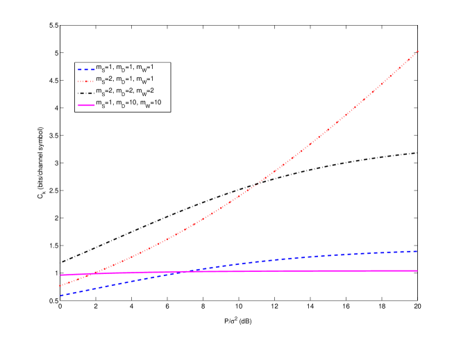
Figure 1: Key capacities of fast-fading MIMO wiretap channels with different numbers of source, destination, eavesdropper antennas. The eavesdropper’s channel gain $\alpha^{2}=0$dB, and $\sigma_{D}^{2}=\sigma_{W}^{2}=\sigma^{2}$.

In Fig. 1, the key capacities of several fast-fading MIMO channels with different number of source, destination, and eavesdropper antennas are plotted against the source signal-to-noise ratio (SNR) $P/\sigma^{2}$ where $\sigma_{D}^{2}=\sigma_{W}^{2}=\sigma^{2}$. The channel gain advantage of the eavesdropper is set to $\alpha^{2}=1$. We observe that the key capacity levels off as $P/\sigma^{2}$ increases in three of the four channels, except the case of $(m_{S},m_{D},m_{W})=(2,1,1)$, considered in Fig. 1. It appears that the relative antenna dimensions determine the asymptotic behavior of the key capacity when the SNR is large. To more precisely study this behavior, we evaluate the limiting value of $C_{K}$ as the input power $P$ of the source becomes very large. To highlight the dependence of $C_{K}$ on $P$, we use the notation $C_{K}(P)$.

Corollary III.1

1. If $m_{W}\geq m_{S}$, then

   $$\lim_{P\rightarrow\infty}C_{K}(P)=E\left[\log\frac{\det\left(H_{W}^{\dagger}H_{W}+\frac{\sigma_{W}^{2}}{\alpha^{2}\sigma_{D}^{2}}H_{D}^{\dagger}H_{D}\right)}{\det\left(H_{W}^{\dagger}H_{W}\right)}\right].$$

2. Suppose that $m_{W}<m_{S}$. Define

   $$C_{\infty}(P)=E\left[\log\det\left(I_{m_{D}}+\frac{P}{m_{S}\sigma_{D}^{2}}H_{D}\left[I_{m_{S}}-H_{W}^{\dagger}\left(H_{W}H_{W}^{\dagger}\right)^{-1}H_{W}\right]H_{D}^{\dagger}\right)\right].$$

   Then $\lim_{P\rightarrow\infty}\frac{C_{K}(P)}{C_{\infty}(P)}=1$.

Proof:

First fix $(\lambda_{1},\lambda_{2},\ldots,\lambda_{m_{S}})=\left(\frac{P}{m_{S}},\frac{P}{m_{S}},\ldots,\frac{P}{m_{S}}\right)$ or equivalently $K_{X}=\frac{P}{m_{s}}I_{m_{S}}$, and consider the mapping $G$ defined in the proof of Lemma III.2 as a function of $P$. Also define

$$\hat{f}(P)=\log\det\left(I_{m_{D}}+\frac{P}{m_{S}\sigma_{D}^{2}}H_{D}\left(I_{m_{S}}+\frac{\alpha^{2}P}{m_{S}\sigma_{W}^{2}}H_{W}^{\dagger}H_{W}\right)^{-1}H_{D}^{\dagger}\right).$$

Thus $C_{K}(P)=E[\hat{f}(P)]$. It is not hard to check that for any $P<\tilde{P}$, $G(\tilde{P})\geq G(P)$, which implies that $\det(G(P))\geq\det(G(\tilde{P}))$. Hence $\hat{f}$ is increasing in $P$. Since the elements of $H_{W}$ are continuously i.i.d., $\mathrm{rank}(H_{W}^{\dagger}H_{W})=\mathrm{rank}(H_{W}H_{W}^{\dagger})=\mathrm{rank}(H_{W})=\min(m_{S},m_{W})$ w.p.1. Thus the matrix $H_{W}^{\dagger}H_{W}$ (resp. $H_{W}H_{W}^{\dagger}$) is invertible w.p.1 when $m_{W}\geq m_{S}$ (resp. $m_{W}<m_{S}$).

Now, consider the case of $m_{W}\geq m_{S}$. As in (21), we have

$$\hat{f}(P)=\log\frac{\det\left(\frac{m_{S}\sigma_{W}^{2}}{\alpha^{2}P}I_{m_{S}}+H_{W}^{\dagger}H_{W}+\frac{\sigma_{W}^{2}}{\alpha^{2}\sigma_{D}^{2}}H_{D}^{\dagger}H_{D}\right)}{\det\left(\frac{m_{S}\sigma_{W}^{2}}{\alpha^{2}P}I_{m_{S}}+H_{W}^{\dagger}H_{W}\right)}.$$

Since $H_{W}^{\dagger}H_{W}$ is invertible w.p.1,

$$\lim_{P\rightarrow\infty}\hat{f}(P)=\log\frac{\det\left(H_{W}^{\dagger}H_{W}+\frac{\sigma_{W}^{2}}{\alpha^{2}\sigma_{D}^{2}}H_{D}^{\dagger}H_{D}\right)}{\det\left(H_{W}^{\dagger}H_{W}\right)}~{}~{}~{}~{}~{}\mbox{w.p.1}.$$

Hence Part 1) of the lemma results from monotone convergence.

For the case of $m_{W}<m_{S}$, the matrix inversion formula allows us to instead write

$$\hat{f}(P)=\log\det\left(I_{m_{D}}+\frac{P}{m_{S}\sigma_{D}^{2}}H_{D}\left[I_{m_{S}}-H_{W}^{\dagger}\left(\frac{m_{S}\sigma_{W}^{2}}{\alpha^{2}P}I_{m_{W}}+H_{W}H_{W}^{\dagger}\right)^{-1}H_{W}\right]H_{D}^{\dagger}\right)$$

Since $H_{W}H_{W}^{\dagger}$ is invertible w.p.1, we can also define

$$\hat{f}_{\infty}(P)=\log\det\left(I_{m_{D}}+\frac{P}{m_{S}\sigma_{D}^{2}}H_{D}\left[I_{m_{S}}-H_{W}^{\dagger}\left(H_{W}H_{W}^{\dagger}\right)^{-1}H_{W}\right]H_{D}^{\dagger}\right).$$

Note that $C_{\infty}(P)=E[\hat{f}_{\infty}(P)]$. Since $H_{W}$ is of rank $m_{W}$ w.p.1, it has the singular value decomposition $H_{W}=U_{W}\left[S_{W}\ 0_{m_{S}-m_{W}}\right]V_{W}^{\dagger}$, where $S_{W}=\mbox{diag}(s_{1},s_{2},\ldots,s_{m_{W}})$ is a diagonal matrix whose diagonal elements are the positive singular values of $H_{W}$. Also let $V=[\tilde{V}\ \hat{V}]$, i.e., $\tilde{V}_{W}$ and $\hat{V}_{W}$ consist respectively of the first $m_{W}$ and the last $m_{S}-m_{W}$ columns of $V$. Employing the unitary property of $U_{W}$ and $V_{W}$, it is not hard to verify that

$$\hat{f}(P) = \log\det\left(I_{m_{D}}+\frac{P}{m_{S}\sigma_{D}^{2}}H_{D}\hat{V}_{W}\hat{V}_{W}^{\dagger}H_{D}^{\dagger}+H_{D}\tilde{V}_{W}\Lambda_{W}(P)\tilde{V}_{W}^{\dagger}H_{D}^{\dagger}\right)$$ (22)

$$\hat{f}_{\infty}(P) = \log\det\left(I_{m_{D}}+\frac{P}{m_{S}\sigma_{D}^{2}}H_{D}\hat{V}_{W}\hat{V}_{W}^{\dagger}H_{D}^{\dagger}\right)$$ (23)

where $\Lambda_{W}(P)=\frac{\sigma_{W}^{2}}{\alpha^{2}\sigma_{D}^{2}}\left(\frac{m_{S}\sigma_{W}^{2}}{\alpha^{2}P}I_{m_{W}}+S_{W}^{2}\right)^{-1}$. From (22) and (23), it is clear that $\hat{f}_{\infty}(P)\leq\hat{f}(P)$.

Further let $t(P)=\mathrm{tr}\left(H_{D}\tilde{V}_{W}\Lambda_{W}(P)\tilde{V}_{W}^{\dagger}H_{D}^{\dagger}\right)$. Since $t(P)I_{m_{D}}\geq H_{D}\tilde{V}_{W}\Lambda_{W}(P)\tilde{V}_{W}^{\dagger}H_{D}^{\dagger}$,

$$\hat{f}(P) \leq \log\det\left([1+t(P)]I_{m_{D}}+\frac{P}{m_{S}\sigma_{D}^{2}}H_{D}\hat{V}_{W}\hat{V}_{W}^{\dagger}H_{D}^{\dagger}\right)$$ (24)

$$= m_{D}\log(1+t(P))+\log\det\left(I_{m_{D}}+\frac{P}{m_{S}\sigma_{D}^{2}[1+t(P)]}H_{D}\hat{V}_{W}\hat{V}_{W}^{\dagger}H_{D}^{\dagger}\right).$$

Let $\mu_{1},\mu_{2},\ldots,\mu_{j}$ be the positive eigenvalues of $H_{D}\hat{V}_{W}\hat{V}_{W}^{\dagger}H_{D}^{\dagger}$. Note that $1\leq j\leq\min(m_{D},m_{S}-m_{W})$, because of the fact that the elements of $H_{D}$ are continuously i.i.d. and are independent of the elements of $H_{W}$. Hence, from (23), (24) and the fact that $\hat{f}_{\infty}(P)\leq\hat{f}(P)$, we have

$$0\ \leq\ \hat{f}(P)-\hat{f}_{\infty}(P) \leq m_{D}\log(1+t(P))+\log\left(\frac{\prod_{i=1}^{j}\left[1+\frac{P\mu_{i}}{m_{S}\sigma_{D}^{2}(1+t(P))}\right]}{\prod_{i=1}^{j}\left[1+\frac{P\mu_{i}}{m_{S}\sigma_{D}^{2}}\right]}\right)$$ (25)

$$= m_{D}\log(1+t(P))+\sum_{i=1}^{j}\log\left(\frac{\frac{1}{1+t(P)}+\frac{m_{S}\sigma_{D}^{2}}{P\mu_{i}}}{1+\frac{m_{S}\sigma_{D}^{2}}{P\mu_{i}}}\right).$$

Now note that

$$\lim_{P\rightarrow\infty}t(P)=\frac{\sigma_{W}^{2}}{\alpha^{2}\sigma_{D}^{2}}\mathrm{tr}\left(H_{D}\tilde{V}_{W}S_{W}^{-2}\tilde{V}_{W}^{\dagger}H_{D}^{\dagger}\right)=\frac{\sigma_{W}^{2}}{\alpha^{2}\sigma_{D}^{2}}\mathrm{tr}\left([H_{W}^{-1}H_{D}^{\dagger}]^{\dagger}H_{W}^{-1}H_{D}^{\dagger}\right)$$

where $H_{W}^{-1}$ denotes the Penrose-Moore pseudo-inverse of $H_{W}$. Then (25) implies that

$$0 \leq \liminf_{P\rightarrow\infty}[\hat{f}(P)-\hat{f}_{\infty}(P)]$$

$$\leq \limsup_{P\rightarrow\infty}[\hat{f}(P)-\hat{f}_{\infty}(P)]$$

$$\leq (m_{D}-j)\log\left(1+\frac{\sigma_{W}^{2}}{\alpha^{2}\sigma_{D}^{2}}\mathrm{tr}\left([H_{W}^{-1}H_{D}^{\dagger}]^{\dagger}H_{W}^{-1}H_{D}^{\dagger}\right)\right)\mbox{~{}~{}~{}~{}~{}w.p.1.}$$

Hence by Fatou’s lemma, we get

$$0 \leq \liminf_{P\rightarrow\infty}[C_{K}(P)-C_{\infty}(P)]$$ (26)

$$\leq \limsup_{P\rightarrow\infty}[C_{K}(P)-C_{\infty}(P)]$$

$$\leq E\left[(m_{D}-j)\log\left(1+\frac{\sigma_{W}^{2}}{\alpha^{2}\sigma_{D}^{2}}\mathrm{tr}\left([H_{W}^{-1}H_{D}^{\dagger}]^{\dagger}H_{W}^{-1}H_{D}^{\dagger}\right)\right)\right].$$

From (23), it is clear that $\hat{f}_{\infty}(P)$ increases without bound in $P$ w.p.1; hence $C_{\infty}(P)$ also increases without bound. Combining this fact with (26), we arrive at the conclusion of Part 2) of the lemma. ∎

Part 1) of the lemma verifies the observations shown in Fig. 1 that the key capacity levels off as the SNR increases if the number of source antennas is no larger than that of eavesdropper antennas. When the source has more antennas, Part 2) of the lemma suggests that the key capacity can grow without bound as $P$ increases similarly to a MIMO fading channel with capacity $C_{\infty}(P)$. Note that the matrix $I_{m_{S}}-H_{W}^{\dagger}\left(H_{W}H_{W}^{\dagger}\right)^{-1}H_{W}$ in the expression that defines $C_{\infty}(P)$ is a projection matrix to the orthogonal complement of the column space of $H_{W}$. Thus $C_{\infty}(P)$ has the physical interpretation that the secret information is passed across the dimensions not observable by the eavesdropper. The most interesting aspect is that this mode of operation can be achieved even if neither the source nor the destination knows the channel matrix $H_{W}$.

We note that the asymptotic behavior of the key capacity in the high SNR regime summarized in Corollary III.1 is similar to the idea of secrecy degree of freedom introduced in [35]. The subtle difference here is that no up-to-date CSI of the destination channel is needed at the source.

Another interesting observation from Fig. 1 is that for the case of $(m_{S},m_{D},m_{W})=(1,10,10)$, the source power $P$ seems to have little effect on the key capacity. A small amount of source power is enough to get close to the leveling key capacity of about $1$ bit per channel use. This observation is generalized below by Corollary III.2, which characterizes the effect of spatial dimensionality of the destination and eavesdropper on the key capacity when the destination and eavesdropper both have a large number of antennas.

Corollary III.2

When $m_{D}$ and $m_{W}$ approaches infinity in such a way that $\displaystyle\lim_{m_{D},m_{W}\rightarrow\infty}\frac{m_{W}}{m_{D}}=\beta$,

$$C_{K}\rightarrow m_{S}\log\left(1+\frac{1}{\beta\alpha^{2}\sigma^{2}_{D}/\sigma^{2}_{W}}\right).$$

Proof:

This corollary is a direct consequence of the fact that $\frac{1}{m_{D}}H_{D}^{\dagger}H_{D}\rightarrow I_{m_{S}}$ and $\frac{1}{m_{W}}H_{W}^{\dagger}H_{W}\rightarrow I_{m_{S}}$ w.p.1, which is in turn due to the strong law of large numbers. ∎

Note that we can interpret the ratio $\beta$ as the spatial dimensionality advantage of the eavesdropper over the destination. The expression for the limiting $C_{K}$ in the corollary clearly indicates that this spatial dimensionality advantage affects the key capacity in the same way as the channel gain advantage $\alpha^{2}$.

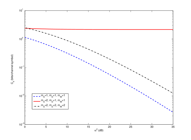
Figure 2: Key capacities of fast-fading MIMO wiretap channels with different numbers of source, destination, eavesdropper antennas. The source signal to noise ratio $P/\sigma^{2}=10$dB, where $\sigma_{D}^{2}=\sigma_{W}^{2}=\sigma^{2}$.

In Fig. 2, the key capacities of several fast-fading MIMO channels with different numbers of source, destination, and eavesdropper antennas are plotted against the eavesdropper’s channel gain advantage $\alpha^{2}$, with $P/\sigma^{2}=10$dB. The results in Fig. 2 show the other effect of spatial dimensionality. We observe that the key capacity decreases almost reciprocally with $\alpha^{2}$ in the channels with $(m_{S},m_{D},m_{W})=(1,1,1)$ and $(m_{S},m_{D},m_{W})=(2,2,2)$, but stays almost constant for the channel with $(m_{S},m_{D},m_{W})=(2,1,1)$. It seems that the relative numbers of source and eavesdropper antennas again play the main role in differentiating these two different behaviors of the key capacity. To verify that, we evaluate the limiting value of $C_{K}$ as the gain advantage $\alpha^{2}$ of the eavesdropper becomes very large. To highlight the dependence of $C_{K}$ on $\alpha^{2}$, we use the notation $C_{K}(\alpha^{2})$.

Corollary III.3

$\lim_{\alpha\rightarrow\infty}C_{K}(\alpha^{2})=\left\{\begin{array}[]{ll}0&\ \mathrm{if}\ m_{W}\geq m_{S}\\ C_{\infty}(P)&\ \mathrm{if}\ m_{W}<m_{S}.\end{array}\right.$

Proof:

Similar to the proof of Corollary III.1. ∎

Similar to the case of large SNR, when the number of source antennas is larger than that of the eavesdropper’s antennas, secret information can be passed across the dimensions not observable by the eavesdropper. This can be achieved with neither the source nor the destination knowing the channel matrix $H_{W}$.

IV Alternative Achievability of Key Capacity

In this section, we provide an alternative proof of achievability for key capacity, which does not require the transmission of continuous symbols over the public channel. We derive the result from “first principles”, which provides more insight on the desirable structure of a practical key agreement scheme. The main steps of the key agreement procedure are the following:

1. the source sends a sequence of i.i.d. symbols $X^{n}$;

2. the destination “quantizes” its received sequence $Y^{n}$ into $\hat{Y}^{n}$ with a Wyner-Ziv compression scheme;

3. the destination uses a binning scheme with the quantized symbol sequences to determine the secret key and the information to feed back to the source over the public channel;

4. the source exploits the information sent by the destination to reconstruct the destination’s quantized sequence $\hat{Y}^{n}$ and uses the same binning scheme to generate its secret key.

The secrecy of the resulting key is established by carefully structuring the binning scheme.

For the memoryless wiretap channel $(X,Y,Z)$ specified by the joint pdf $p(y|x)p(z|x)p(x)$, consider the quadruple $(X,Y,\hat{Y},Z)$ defined by the joint pdf $p(x,y,\hat{y},z)=p(\hat{y}|y)p(y|x)p(z|x)p(x)$ with $p(\hat{y}|y)$ to be specified later. We assume that $\hat{Y}$ takes values in the alphabet $\mathcal{Y}$. Given a sequence of $n$ elements $x_{n}=(x_{1},x_{2},\ldots,x_{n})$, $p(x^{n})=\prod_{j=1}^{n}p(x_{j})$ unless otherwise specified. Similar notation and convention apply to all other sequences as well as their corresponding pdfs and conditional pdfs considered hereafter.

IV-A Random Code Generation

Choose $p(\hat{y}|y)$ such that $I(X;\hat{Y})-I(\hat{Y};Z)>0$ and $I(\hat{Y};Z)>0$, and let $p(\hat{y})$ denote the corresponding marginal. Note that the existence of such $p(\hat{y}|y)$ can be assumed without loss of generality if $I(X;Y)-I(Y;Z)>0$ and $I(Y;Z)>0$. If $I(X;Y)-I(Y;Z)=0$, there is nothing to prove. Similarly, if $I(Y;Z)=0$, the construction below can be trivially modified to show that $I(X;Y)$ is an achievable key rate.

Fix a small (small enough so that the various rate definitions and bounds on probabilities below make sense and are non-trivial) $\varepsilon>0$. Let us define

$$R_{1} \stackrel{{\scriptstyle\Delta}}{{=}} I(Y;\hat{Y})+4\varepsilon$$

$$R_{2} \stackrel{{\scriptstyle\Delta}}{{=}} I(Y;\hat{Y})-I(X;\hat{Y})+22\varepsilon$$

$$R_{3} \stackrel{{\scriptstyle\Delta}}{{=}} I(X;\hat{Y})-I(\hat{Y};Z)-\varepsilon$$

$$R_{4} \stackrel{{\scriptstyle\Delta}}{{=}} I(\hat{Y};Z)-17\varepsilon.$$ (27)

For each $j=1,2,\ldots,2^{nR_{2}}$ and $l=1,2,\ldots,2^{nR_{3}}$, generate $2^{nR_{4}}$ codewords $\hat{Y}^{n}(j,l,1),\hat{Y}^{n}(j,l,2),\ldots,\hat{Y}^{n}(j,l,2^{nR_{4}})$ according to $p(\hat{y}^{n})$. The set of codewords $\{\hat{Y}^{n}(j,l,k)\}$ with ${k=1\dots 2^{nR_{4}}}$ forms a subcode denoted by $\mathcal{C}(j,l)$. The union of all subcodes $\mathcal{C}(j,l)$ for $j=1,2,\ldots,2^{nR_{2}}$ and $l=1,2,\ldots,2^{nR_{3}}$ forms the code $\mathcal{C}$. For convenience, we denote the $2^{nR_{1}}$ codewords in $\mathcal{C}$ as $\hat{Y}^{n}(1),\hat{Y}^{n}(2),\ldots,\hat{Y}^{n}(2^{nR_{1}})$, where $\hat{Y}^{n}(j+(l-1)2^{nR_{2}}+(w-1)2^{n(R_{2}+R_{3})})=\hat{Y}^{n}(j,l,w)$ for $j=1,2,\ldots,2^{nR_{2}}$, $l=1,2,\ldots,2^{nR_{3}}$, and $w=1,2,\ldots,2^{nR_{4}}$. The code $\mathcal{C}$ and its subcodes $\mathcal{C}(j,l)$ is revealed to the source, destination, and eavesdropper. In the following, we refer to a codeword or its index in $\mathcal{C}$ interchangeably. Under this convention, the subcode $\mathcal{C}(j,l)$ is also the set that contains all the indices of its codewords. Denote $\mathcal{\hat{C}}(j)=\bigcup_{l=1}^{2^{nR_{3}}}\mathcal{C}(j,l)$ and $\mathcal{\tilde{C}}(l)=\bigcup_{j=1}^{2^{nR_{2}}}\mathcal{C}(j,l)$.

IV-B Secret Sharing Procedure

For convenience, we define the joint typicality indicator function $T_{\varepsilon}(\cdot)$ that takes in a number of sequences as its arguments. The value of $T_{\varepsilon}(\cdot)$ is $1$ if the sequences are $\varepsilon$-jointly typical, and the value is $0$ otherwise. Further define the indicator function for the sequence pair $(y^{n},\hat{y}^{n})$:

$$S_{\varepsilon}(y^{n},\hat{y}^{n})=\left\{\begin{array}[]{ll}1&\ \mathrm{if}\ \Pr\{T_{\varepsilon}(X^{n},y^{n},\hat{y}^{n},Z^{n})=1\}\geq 1-\varepsilon\\ 0&\ \mathrm{otherwise}\end{array}\right.$$

where $(X^{n},Z^{n})$ is distributed according to $p(x^{n},z^{n}|y^{n},\hat{y}^{n})$ in the definition above.

The source generates a random sequence $X^{n}$ distributed according to $p(x^{n})$. If $X^{n}$ satisfies the average power constraint (1), the source sends $X^{n}$ through the $(X,Y,Z)$ channel. Otherwise, it ends the secret-sharing process. Since $p(x)$ satisfies $E[|X|^{2}]\leq P$, the law of large numbers implies that the probability of the latter event can be made arbitrarily small by increasing $n$. Hence we can assume below, with no loss of generality, that $X^{n}$ satisfies (1) and is sent by the source. This assumption helps to make the probability calculations in Section IV-C less tedious.

Upon reception of the sequence $Y^{n}$, the destination tries to quantize the received sequence. Let $M$ be the output of its quantizer. Specifically, if there is a unique sequence $\hat{Y}^{n}(m)\in\mathcal{C}$ for some $m\in\{1,2,\ldots,2^{nR_{1}}\}$ such that $S_{\varepsilon}(Y^{n},\hat{Y}^{n}(m))=1$, then it sets the output of the quantizer to $M=m$. If there is more than one such sequence, $M$ is set to be the smallest sequence index $m$. If there is no such sequence, it sets $M=0$. Let $L$ and $J$ be the unique indices such that $\hat{Y}^{n}(M)\in\mathcal{C}(J,L)$. The index $L$ will be used as the key while the index $J$ is fed back to the source over the public channel, i.e. $\Psi_{k}=J$. If $M=0$, set $J=0$ and choose $L$ randomly over $\{1,2,\ldots,2^{nR_{3}}\}$ with uniform probabilities.

After receiving the feedback information $J$ via the public channel, the source attempts to find a unique $\hat{Y}^{n}(m)\in\mathcal{C}$ such that $T_{\varepsilon}(X^{n},\hat{Y}^{n}(m))=1$ and $m\in\mathcal{\hat{C}}(J)$. If there is such a unique $\hat{Y}^{n}(m)$, the source decodes $\hat{M}=m$. If there is no such sequence or more than one such sequence, the source sets $\hat{M}=0$. If $J=0$, it sets $\hat{M}=0$. Finally, if $\hat{M}>0$, the source generates its key $K=k$, such that $\hat{M}\in\mathcal{C}(J,k)$. If $\hat{M}=0$, it sets $K=0$.

We also consider a fictitious receiver who observes the sequence $Z^{n}$ and obtains both indices $J$ and $L$ via the public channel. This receiver sets $\tilde{M}=0$ if $J=0$. Otherwise, it attempts to find a unique $\hat{Y}^{n}(m)\in\mathcal{C}$ such that $T_{\varepsilon}(\hat{Y}^{n}(m),Z^{n})=1$ and $m\in\mathcal{C}(J,L)$. If there is such a unique $\hat{Y}^{n}(m)$, the source decodes $\tilde{M}=m$. If there is no such sequence or more than one such sequence, the source sets $\tilde{M}=0$.

IV-C Analysis of Probability of Error

We use a random coding argument to establish the existence of a code with rates given by (27) such that $\Pr\{K\neq L\}$ and $\Pr\{M\neq\tilde{M}\}$ vanish in the limit of large block length $n$. Without further clarification, we note that the probabilities of the events below, except otherwise stated, are over the joint distribution of the codebook $\mathcal{C}$, codewords, and all other random quantities involved.

Before we proceed, we introduce the following lemma regarding the indicator function $S_{\varepsilon}$.

Lemma IV.1

1. If $(Y^{n},\hat{Y}^{n})$ distributes according to $p(y^{n},\hat{y}^{n})$, then $\Pr\{S_{\varepsilon}(Y^{n},\hat{Y}^{n})=1\}>1-\varepsilon$ for sufficiently large $n$.

2. If $\hat{Y}^{n}$ distributes according to $p(\hat{y}^{n})$, then $\Pr\{S_{\varepsilon}(y^{n},\hat{Y}^{n})=1\}\leq\frac{2^{-n(R_{1}-7\varepsilon)}}{1-\varepsilon}$ for all $y^{n}$.

3. If $Y^{n}$ distributes according to $p(y^{n})$, then $\Pr\{S_{\varepsilon}(Y^{n},\hat{y}^{n})=1\}\leq\frac{2^{-n(R_{1}-7\varepsilon)}}{1-\varepsilon}$ for all $\hat{y}^{n}$.

4. If $(Y^{n},\hat{Y}^{n})$ distributes according to $p(y^{n})p(\hat{y}^{n})$, then $\Pr\{S_{\varepsilon}(Y^{n},\hat{Y}^{n})=1\}>(1-\varepsilon)\cdot 2^{-n(R_{1}-\varepsilon)}$ for sufficiently large $n$.

Proof:

1. This claim is actually shown in [36]. We briefly sketch the proof here using our notation for completeness and easy reference. By the reverse Markov inequality [36],

   $$\Pr\{S_{\varepsilon}(Y^{n},\hat{Y}^{n})=1\}\geq 1-\frac{1-\Pr\{T_{\varepsilon}(X^{n},Y^{n},\hat{Y}^{n},Z^{n})=1\}}{1-(1-\varepsilon)}>1-\varepsilon$$

   where the second inequality is due to that fact that $\Pr\{T_{\varepsilon}(X^{n},Y^{n},\hat{Y}^{n},Z^{n})=1\}>1-\varepsilon^{2}$ for sufficiently large $n$.

2. First, we only need to consider typical $y^{n}$ since the bound is trivial when $y^{n}$ is not typical. Notice that for any such $y^{n}$,

   $$1 \geq \int T_{\varepsilon}(x^{n},y^{n},\hat{y}^{n},z^{n})p(x^{n},\hat{y}^{n},z^{n}|y^{n})dx^{n}dz^{n}d\hat{y}^{n}$$

   $$= \int\Pr\{T_{\varepsilon}(X^{n},y^{n},\hat{y}^{n},Z^{n})=1\}\cdot\frac{p(y^{n},\hat{y}^{n})}{p(y^{n})}d\hat{y}^{n}$$

   $$\geq \int\Pr\{T_{\varepsilon}(X^{n},y^{n},\hat{y}^{n},Z^{n})=1\}\cdot\frac{2^{-n(h(Y,\hat{Y})+\varepsilon)}}{2^{-n(h(Y)-\varepsilon)}}d\hat{y}^{n}$$

   $$= 2^{-n(h(\hat{Y}|Y)+2\varepsilon)}\int\Pr\{T_{\varepsilon}(X^{n},y^{n},\hat{y}^{n},Z^{n})=1\}d\hat{y}^{n}.$$

   Hence

   $$2^{n(h(\hat{Y}|Y)+2\varepsilon)} \geq \int\Pr\{T_{\varepsilon}(X^{n},y^{n},\hat{y}^{n},Z^{n})=1\}d\hat{y}^{n}$$ (28)

   $$\geq \int S_{\varepsilon}(y^{n},\hat{y}^{n})\cdot\Pr\{T_{\varepsilon}(X^{n},y^{n},\hat{y}^{n},Z^{n})=1\}d\hat{y}^{n}$$

   $$\geq (1-\varepsilon)\int S_{\varepsilon}(y^{n},\hat{y}^{n})d\hat{y}^{n}.$$

   Now

   $$\Pr\{S_{\varepsilon}(y^{n},\hat{Y}^{n})=1\} = \int S_{\varepsilon}(y^{n},\hat{y}^{n})p(\hat{y}^{n})d\hat{y}^{n}$$

   $$\leq \int S_{\varepsilon}(y^{n},\hat{y}^{n})2^{-n(h(\hat{Y})-\varepsilon)}d\hat{y}^{n}$$

   $$\leq \frac{2^{-n(I(Y;\hat{Y})-3\varepsilon)}}{1-\varepsilon},$$

   where the last inequality is due to (28).

3. Same as Part 2), interchanging the roles of $y^{n}$ and $\hat{y}^{n}$.

4. From Part 1), we get

   $$1-\varepsilon < \int S_{\varepsilon}(y^{n},\hat{y}^{n})p(y^{n},\hat{y}^{n})dy^{n}d\hat{y}^{n}$$

   $$= \int S_{\varepsilon}(y^{n},\hat{y}^{n})\frac{p(y^{n},\hat{y}^{n})}{p(y^{n})p(\hat{y}^{n})}p(y^{n})p(\hat{y}^{n})dy^{n}d\hat{y}^{n}$$

   $$\leq \int S_{\varepsilon}(y^{n},\hat{y}^{n})\cdot\frac{2^{-n(h(Y,\hat{Y})-\varepsilon)}}{2^{-n(h(Y)+\varepsilon)}\cdot 2^{-n(h(\hat{Y})+\varepsilon)}}\cdot p(y^{n})p(\hat{y}^{n})dy^{n}d\hat{y}^{n}$$

   $$= 2^{n(I(Y;\hat{Y})-3\varepsilon)}\Pr\{S_{\varepsilon}(Y^{n},\hat{Y}^{n})=1\}.$$

∎

Moreover we need to bound the probabilities of the following events pertaining to $M$.

Lemma IV.2

1. $\Pr\{M=0\}<2\varepsilon$ for sufficiently large $n$.

2. For $m=1,2,\ldots,2^{nR_{1}}$, $\Pr\{M=m\}\leq\frac{2^{-n(R_{1}-7\varepsilon)}}{1-\varepsilon}$.

3. When $n$ is sufficiently large, $\Pr\{M=m\}\geq\left[1-\frac{2^{-n(R_{1}-7\varepsilon)}}{1-\varepsilon}\right]^{m-1}\cdot(1-\varepsilon)2^{-n(R_{1}-\varepsilon)}$ uniformly for all $m=1,2,\ldots,2^{nR_{1}}$.

4. When $n$ is sufficiently large, $\Pr\{J=j,L=l\}>(1-\varepsilon)^{4}\cdot 2^{-n(R_{1}-R_{4}+6\varepsilon)}$ uniformly for all $j=1,2,\ldots,2^{nR_{2}}$ and $l=1,2,\ldots,2^{nR_{3}}$.

Proof:

1. We will use an argument similar to the one in the achievability proof of rate distortion function in [27, Section 10.5] to bound $\Pr\{M=0\}$. First note that $\{M=0\}$ is the event that $S_{\varepsilon}(Y^{n},\hat{Y}^{n}(m))=0$ for all $m\in\{1,2,\ldots,R_{1}\}$, and hence

   $$\Pr\{M=0\} = \Pr\left\{\bigcap_{m=1}^{2^{nR_{1}}}\{S_{\varepsilon}(Y^{n},\hat{Y}^{n}(m))=0\}\right\}$$ (29)

   $$= \int\left[\Pr\{S_{\varepsilon}(y^{n},\hat{Y}^{n}(1))=0\}\right]^{2^{nR_{1}}}p(y^{n})dy^{n},$$

   where the second equality is due to the fact that $\hat{Y}^{n}(1),\ldots,\hat{Y}^{n}(2^{nR_{1}})$ are i.i.d. given each fixed $y^{n}$. But

   $$\left[\Pr\{S_{\varepsilon}(y^{n},\hat{Y}^{n}(1))=0\}\right]^{2^{nR_{1}}} = \left[1-\int S_{\varepsilon}(y^{n},\hat{y}^{n})p(\hat{y}^{n})d\hat{y}^{n}\right]^{2^{nR_{1}}}$$ (30)

   $$= \left[1-\int S_{\varepsilon}(y^{n},\hat{y}^{n})p(\hat{y}^{n}|y^{n})\frac{p(y^{n})p(\hat{y}^{n})}{p(y^{n},\hat{y}^{n})}d\hat{y}^{n}\right]^{2^{nR_{1}}}$$

   $$\leq \left[1-\int S_{\varepsilon}(y^{n},\hat{y}^{n})p(\hat{y}^{n}|y^{n})\frac{2^{-n(h(Y)+\varepsilon)}\cdot 2^{-n(h(\hat{Y})+\varepsilon)}}{2^{-n(h(Y,\hat{Y})-\varepsilon)}}d\hat{y}^{n}\right]^{2^{nR_{1}}}$$

   $$= \left[1-2^{-n(I(Y;\hat{Y})+3\varepsilon)}\int S_{\varepsilon}(y^{n},\hat{y}^{n})p(\hat{y}^{n}|y^{n})d\hat{y}^{n}\right]^{2^{nR_{1}}}$$

   $$\leq 1-\int S_{\varepsilon}(y^{n},\hat{y}^{n})p(\hat{y}^{n}|y^{n})d\hat{y}^{n}+\exp\left(-2^{n\varepsilon}\right),$$

   where the inequality on the third line is due to the fact that $S_{\varepsilon}(y^{n},\hat{y}^{n})=1$ implies $T_{\varepsilon}(y^{n},\hat{y}^{n})=1$, and the last line results from the inequality $(1-xy)^{k}\leq 1-x+e^{-ky}$ for all $0\leq x,y\leq 1$ and positive integer $k$ [27, Lemma 10.5.3]. Substituting (30) back into (29) and using Lemma IV.1 Part 1), we get

   $$\Pr\{M=0\}\leq 1-\Pr\{S_{\varepsilon}(Y^{n},\hat{Y}^{n})=1\}+\exp\left(-2^{n\varepsilon}\right)<\varepsilon+\varepsilon=2\varepsilon$$

   for sufficiently large $n$.

2. Notice that for $m=1,2,\ldots,2^{nR_{1}}$,

   $$\Pr\{M=m\} = \Pr\{S_{\varepsilon}(Y^{n},\hat{Y}^{n}(m))=1,S_{\varepsilon}(Y^{n},\hat{Y}^{n}(m-1))=0,\ldots,S_{\varepsilon}(Y^{n},\hat{Y}^{n}(1))=0\}$$ (31)

   $$= \int\Pr\{S_{\varepsilon}(y^{n},\hat{Y}^{n}(1))=1\}\left[\Pr\{S_{\varepsilon}(y^{n},\hat{Y}^{n}(1))=0\}\right]^{m-1}p(y^{n})dy^{n}$$

   where the second equality results from the i.i.d. nature of $\hat{Y}^{n}(1),\ldots,\hat{Y}^{n}(m)$. Thus we have

   $$\Pr\{M=m\}\leq\Pr\{S_{\varepsilon}(Y^{n},\hat{Y}^{n}(1))=1\}\leq\frac{2^{-n(R_{1}-7\varepsilon)}}{1-\varepsilon},$$

   where the last inequality is due to Part 2) of Lemma IV.1 since $Y^{n}$ and $\hat{Y}^{n}(1)$ are independent.

3. From (31), we have the lower bound

   $$\Pr\{M=m\} \geq \left[1-\frac{2^{-n(R_{1}-7\varepsilon)}}{1-\varepsilon}\right]^{m-1}\Pr\{S_{\varepsilon}(Y^{n},\hat{Y}^{n}(1))=1\}$$

   $$\geq \left[1-\frac{2^{-n(R_{1}-7\varepsilon)}}{1-\varepsilon}\right]^{m-1}\cdot(1-\varepsilon)2^{-n(R_{1}-\varepsilon)}$$

   where the first inequality is due to Part 2) of Lemma IV.1, and the second inequality is from Part 4) of Lemma IV.1 when $n$ is sufficiently large. Note that the same sufficiently large $n$ is enough to guarantee the validity of the lower bound above for all $m=1,2,\ldots,2^{nR_{1}}$.

4. First note that, for $j=1,2,\ldots,2^{nR_{2}}$ and $l=1,2,\ldots,2^{nR_{3}}$,

   $$\Pr\{J=j,L=l\}=\sum_{m\in\mathcal{C}(j,l)}\Pr\{M=m\}=\sum_{w=1}^{2^{nR_{4}}}\Pr\left\{M=j+(l-1)2^{nR_{2}}+(w-1)2^{n(R_{2}+R_{3})}\right\}.$$

   Thus applying Part 3) of the lemma, we get

   $$\Pr\{J=j,L=l\}$$ (32)

   $$\geq (1-\varepsilon)2^{-n(R_{1}-\varepsilon)}\cdot\sum_{w=1}^{2^{nR_{4}}}\left[1-\frac{2^{-n(R_{1}-7\varepsilon)}}{1-\varepsilon}\right]^{j-1+(l-1)2^{nR_{2}}+(w-1)2^{n(R_{2}+R_{3})}}$$

   $$\geq (1-\varepsilon)2^{-n(R_{1}-\varepsilon)}\left[1-\frac{2^{-n(R_{1}-7\varepsilon)}}{1-\varepsilon}\right]^{2^{n(R_{2}+R_{3})}}\frac{1-\left[1-2^{-n(R_{1}-7\varepsilon)}/(1-\varepsilon)\right]^{2^{nR_{1}}}}{1-\left[1-2^{-n(R_{1}-7\varepsilon)}/(1-\varepsilon)\right]^{2^{n(R_{2}+R_{3})}}}$$

   $$\geq (1-\varepsilon)2^{-n(R_{1}-\varepsilon)}\left[1-\frac{2^{-n(R_{4}-7\varepsilon)}}{1-\varepsilon}\right]\cdot\frac{1-\left[1-2^{-n(R_{1}-7\varepsilon)}/(1-\varepsilon)\right]^{2^{nR_{1}}}}{1-\left[1-2^{-n(R_{4}-7\varepsilon)}/(1-\varepsilon)\right]}$$

   $$\geq (1-\varepsilon)^{2}\cdot 2^{-n(R_{1}-R_{4}+6\varepsilon)}\left[1-\frac{2^{-n(R_{4}-7\varepsilon)}}{1-\varepsilon}\right]\left[1-\frac{\exp(-2^{7n\varepsilon})}{1-\varepsilon}\right]$$

   $$> (1-\varepsilon)^{4}\cdot 2^{-n(R_{1}-R_{4}+6\varepsilon)}$$

   uniformly for all $j=1,2,\ldots,2^{nR_{2}}$ and $l=1,2,\ldots,2^{nR_{3}}$, when $n$ is sufficiently large. The lower bound on the fourth line of (32) above is obtained from the inequality $(1-x)^{k}\geq 1-kx$ for any $0\leq x\leq 1$ and positive integer $k$. The lower bound on the fifth line is in turn based on the inequality $(1-x)^{k}\leq e^{-kx}$ for $0\leq x\leq 1$ and positive integer $k$.

∎

We first consider the error event $\{K\neq L\}$. Note that

$$\Pr\{K\neq L\} = \Pr\{M=0\}+\Pr\{M>0,K\neq L\}$$ (33)

$$= \Pr\{M=0\}+\sum_{m=1}^{2^{nR_{1}}}\Pr\left\{\mathcal{\tilde{E}}_{m}\cup\mathcal{E}_{m},M=m\right\}$$

$$\leq \Pr\{M=0\}+\sum_{m=1}^{2^{nR_{1}}}\Pr\left\{\mathcal{\tilde{E}}_{m},M=m\right\}+\sum_{m=1}^{2^{nR_{1}}}\Pr\left\{\mathcal{E}_{m},M=m\right\}$$

where $\mathcal{\tilde{E}}_{m}$ is the event $\{T_{\varepsilon}(X^{n},\hat{Y}^{n}(m))=0\}$, and $\mathcal{E}_{m}$ is the event that there is an $m^{\prime}\in\mathcal{\hat{C}}(j)$ such that $m\in\mathcal{\hat{C}}(j)$, $m^{\prime}\neq m$, and $T_{\varepsilon}(X^{n},\hat{Y}^{n}(m^{\prime}))=1$. From (31), we have

$$\Pr\left\{\mathcal{\tilde{E}}_{m},M=m\right\}$$ (34)

$$= \Pr\left\{T_{\varepsilon}(X^{n},\hat{Y}^{n}(m))=0,S_{\varepsilon}(Y^{n},\hat{Y}^{n}(m))=1,S_{\varepsilon}(Y^{n},\hat{Y}^{n}(m-1))=0,\ldots,S_{\varepsilon}(Y^{n},\hat{Y}^{n}(1))=0\right\}$$

$$\leq \Pr\Big{\{}T_{\varepsilon}(X^{n},Y^{n},\hat{Y}^{n}(m),Z^{n})=0,S_{\varepsilon}(Y^{n},\hat{Y}^{n}(m))=1,$$

$$~{}~{}~{}~{}~{}~{}~{}~{}S_{\varepsilon}(Y^{n},\hat{Y}^{n}(m-1))=0,\ldots,S_{\varepsilon}(Y^{n},\hat{Y}^{n}(1))=0\Big{\}}$$

$$= \int\left[\int\Pr\left\{T_{\varepsilon}(x^{n},y^{n},\hat{Y}^{n}(m),z^{n})=0,S_{\varepsilon}(y^{n},\hat{Y}^{n}(m))=1\right\}p(x^{n},z^{n}|y^{n})dx^{n}dz^{n}\right]$$

$$~{}~{}~{}~{}~{}~{}\cdot\prod_{m^{\prime}=1}^{m-1}\Pr\{S_{\varepsilon}(y^{n},\hat{Y}^{n}(m^{\prime}))=0\}p(y^{n})dy^{n}$$

$$= \int\left(\left\{\int[1-T_{\varepsilon}(x^{n},y^{n},\hat{y}^{n},z^{n})]p(x^{n},z^{n}|y^{n},\hat{y}^{n})dx^{n}dz^{n}\right\}\cdot S_{\varepsilon}(y^{n},\hat{y}^{n})p(\hat{y}^{n})d\hat{y}^{n}\right)$$

$$~{}~{}~{}~{}~{}~{}\cdot\prod_{m^{\prime}=1}^{m-1}\Pr\{S_{\varepsilon}(y^{n},\hat{Y}^{n}(m^{\prime}))=0\}p(y^{n})dy^{n}$$

$$\leq \varepsilon\cdot\Pr\left\{S_{\varepsilon}(Y^{n},\hat{Y}^{n}(m))=1,S_{\varepsilon}(Y^{n},\hat{Y}^{n}(m-1))=0,\ldots,S_{\varepsilon}(Y^{n},\hat{Y}^{n}(1))=0\right\}$$

$$= \varepsilon\cdot\Pr\{M=m\},$$

where the equality on the fourth line is due to the i.i.d. nature of $\hat{Y}^{n}(1),\ldots,\hat{Y}^{n}(2^{nR_{1}})$, the equality on the fifth line results from the fact that $p(x^{n},z^{n}|y^{n})=p(x^{n},z^{n}|y^{n},\hat{y}^{n})$ (since $(X,Z)\rightarrow Y\rightarrow\hat{Y}$), and the inequality on the second last line is from the definition of the indicator function $S_{\varepsilon}$.

Similarly assuming $m\in\mathcal{\hat{C}}(j)$, we have from (31)

$$\Pr\{\mathcal{E}_{m},M=m\} \leq \sum_{\tiny\begin{array}[]{c}m^{\prime}\in\mathcal{\hat{C}}(j)\\ m^{\prime}\neq m\end{array}}\Pr\left\{T_{\varepsilon}(X^{n},\hat{Y}^{n}(m^{\prime}))=1,S_{\varepsilon}(Y^{n},\hat{Y}^{n}(m))=1\right\}$$ (37)

$$= \sum_{\tiny\begin{array}[]{c}m^{\prime}\in\mathcal{\hat{C}}(j)\\ m^{\prime}\neq m\end{array}}\int\Pr\{T_{\varepsilon}(x^{n},\hat{Y}^{n}(m^{\prime}))=1\}\cdot\Pr\{S_{\varepsilon}(y^{n},\hat{Y}^{n}(m))=1\}p(x^{n},y^{n})dx^{n}dy^{n}$$ (40)

$$\leq 2^{n(R_{1}-R_{2})}\cdot 2^{-n(I(X;\hat{Y})-3\varepsilon)}\cdot\frac{2^{-n(R_{1}-7\varepsilon)}}{1-\varepsilon}=\frac{2^{-n(R_{1}+8\varepsilon)}}{1-\varepsilon},$$ (41)

where the equality on the second line is due to the independence between $\hat{Y}^{n}(m^{\prime})$ and $\hat{Y}^{n}(m)$, and the last inequality results from Part 2) of Lemma IV.1 and the bound $\Pr\{T_{\varepsilon}(x^{n},\hat{Y}^{n}(m^{\prime}))=1\}\leq 2^{-n(I(X;\hat{Y})-3\varepsilon)}$, which is a direct result of [27, Theorem 15.2.2]. Hence, substituting the bounds in (34) and (41) back into (33) and using Part 1) of Lemma IV.2, we obtain

$$\Pr\{K\neq L\}\leq 2\varepsilon+\varepsilon\cdot\sum_{m=1}^{2^{nR_{1}}}\Pr\{M=m\}+\sum_{m=1}^{2^{nR_{1}}}\frac{2^{-n(R_{1}+8\varepsilon)}}{1-\varepsilon}=2\varepsilon+\varepsilon+\frac{2^{-8n\varepsilon}}{1-\varepsilon}<4\varepsilon$$ (42)

for $n$ is sufficiently large.

Next we consider the event $\{M\neq\tilde{M}\}$. Define $\mathcal{\tilde{F}}_{m}$ as the event $\{T_{\varepsilon}(\hat{Y}^{n}(m),Z^{n})=0\}$ and $\mathcal{F}_{m}$ as the event that there is an $m^{\prime}\in\mathcal{C}(l,j)$ such that $m\in\mathcal{C}(l,j)$, $m^{\prime}\neq m$, and $T_{\varepsilon}(\hat{Y}^{n}(m^{\prime}),Z^{n})=1$. Then we have, when $n$ is sufficiently large, uniformly for all $j=1,2,\ldots,2^{nR_{2}}$ and $l=1,2,\ldots,2^{nR_{3}}$,

$$\Pr\{\tilde{M}\neq M|J=j,L=l\}$$ (43)

$$\leq \sum_{m\in\mathcal{C}(j,l)}\Pr\left\{\mathcal{\tilde{F}}_{m},M=m|J=j,L=l\right\}+\sum_{m\in\mathcal{C}(j,l)}\Pr\left\{\mathcal{F}_{m},M=m|J=j,L=l\right\}$$

$$\leq \sum_{m\in\mathcal{C}(j,l)}\varepsilon\cdot\Pr\{M=m|J=j,L=l\}+\sum_{m\in\mathcal{C}(j,l)}\frac{2^{-n(R_{1}+7\varepsilon)}}{1-\varepsilon}\cdot\frac{1}{\Pr\{J=j,L=l\}}$$

$$\leq \varepsilon+\frac{2^{-n(R_{1}+7\varepsilon)}}{1-\varepsilon}\cdot\frac{2^{nR_{4}}}{(1-\varepsilon)^{4}\cdot 2^{-n(R_{1}-R_{4}+6\varepsilon)}}$$

$$= \varepsilon+\frac{2^{-n\varepsilon}}{(1-\varepsilon)^{5}}<2\varepsilon.$$

Note that the inequality on the third line of (43) results from upper bounds of $\Pr\{\mathcal{\tilde{F}}_{m},M=m\}$ and $\Pr\{\mathcal{F}_{m},M=m\}$, which can be obtained in ways almost identical to the derivations in (34) and (41) respectively. The inequality on the fourth line is, on the other hand, due to Part 4) of Lemma IV.2.

By expurgating the random code ensemble, we obtain the following lemma.

Lemma IV.3

For any $\epsilon>0$ and $n$ sufficiently large, there exists a code $\mathcal{C}_{n}$ with the rates $R_{1}$, $R_{2}$, $R_{3}$, and $R_{4}$ given by (27) such that

1. $\Pr\{K\neq L|\mathcal{C}=\mathcal{C}_{n}\}<8\varepsilon$,

2. $\Pr\{M\neq\tilde{M}|\mathcal{C}=\mathcal{C}_{n}\}<8\varepsilon$,

3. $\Pr\{M=m|\mathcal{C}=\mathcal{C}_{n}\}\leq\frac{2^{-n(R_{1}-7\varepsilon)}}{1-\varepsilon}$ for all $m=1,2,\ldots,2^{nR_{1}}$, and

4. $\Pr\{L=l|\mathcal{C}=\mathcal{C}_{n}\}<2^{-n(R_{3}-8\varepsilon)}$ for all $l=1,2,\ldots,2^{nR_{3}}$.

Proof:

Combining Part 1) of Lemma IV.2, (42), and (43), we have

$$\Pr\{M=0\}+\Pr\{K\neq L\}+\Pr\{M\neq\tilde{M}\}<8\varepsilon$$

for sufficiently large $n$. This implies that there must exist a $\mathcal{C}_{n}$ satisfying $\Pr\{K\neq L|\mathcal{C}=\mathcal{C}_{n}\}<8\varepsilon$, $\Pr\{M\neq\tilde{M}|\mathcal{C}=\mathcal{C}_{n}\}<8\varepsilon$, and $\Pr\{M=0|\mathcal{C}=\mathcal{C}_{n}\}<8\varepsilon$. Thus, Parts 1) and 2) are proved.

Now, fix this $\mathcal{C}_{n}$. For $m=1,2,\ldots,2^{nR_{1}}$, let $\hat{y}^{n}(m)$ be the $m$th codeword of $\mathcal{C}_{n}$. Then, by Part 3) of Lemma IV.1,

$$\Pr\{M=m|\mathcal{C}=\mathcal{C}_{n}\}\leq\Pr\{S_{\varepsilon}(Y^{n},\hat{y}^{n}(m))=1\}\leq\frac{2^{-n(R_{1}-7\varepsilon)}}{1-\varepsilon};$$

hence, Part 3) results.

Note that, for $l=1,2,\ldots,2^{nR_{3}}$,

$$\Pr\{L=l|\mathcal{C}=\mathcal{C}_{n}\}=\Pr\{L=l|M=0,\mathcal{C}=\mathcal{C}_{n}\}\Pr\{M=0|\mathcal{C}=\mathcal{C}_{n}\}+\Pr\{L=l,M>0|\mathcal{C}=\mathcal{C}_{n}\}.$$ (44)

We know from the discussion above that $\Pr\{L=l|M=0,\mathcal{C}=\mathcal{C}_{n}\}\Pr\{M=0|\mathcal{C}=\mathcal{C}_{n}\}<2^{-nR_{3}}\cdot 8\varepsilon$. Also from Part 3) of the lemma,

$$\Pr\{L=l,M>0|\mathcal{C}=\mathcal{C}_{n}\}=\sum_{m\in\mathcal{\tilde{C}}_{n}(l)}\Pr\{M=m|\mathcal{C}=\mathcal{C}_{n}\}\leq 2^{n(R_{1}-R_{3})}\cdot\frac{2^{-n(R_{1}-7\varepsilon)}}{1-\varepsilon}=\frac{2^{-n(R_{3}-7\varepsilon)}}{1-\varepsilon}.$$

Putting these back into (44), we get

$$\Pr\{L=l|\mathcal{C}=\mathcal{C}_{n}\}<2^{-n(R_{3}-7\varepsilon)}\left[8\varepsilon\cdot 2^{-7n\varepsilon}+\frac{1}{1-\varepsilon}\right]<2^{-n(R_{3}-8\varepsilon)}$$

for sufficiently large $n$. Thus, Part 4) is proved. ∎

In the remainder of the paper, we use a fixed code $\mathcal{C}_{n}$ identified by Lemma IV.3. For convenience, we drop the conditioning on $\mathcal{C}_{n}$.

IV-D Secrecy Analysis

First we proceed to bound $H(K)$. Note that

$$H(K) = H(L)+H(K|L)-H(L|K)$$ (45)

$$\geq H(L)-H(L|K).$$

Using Part 1) of Lemma IV.3 together with Fano’s inequality gives $H(L|K)\leq 1+8n\varepsilon R_{3}$. Moreover Part 4) of Lemma IV.3 implies that $H(L)>n(R_{3}-8\varepsilon)$. Putting these bounds back into (45), we have

$$R_{3}-(8R_{3}+8)\varepsilon-\frac{1}{n}<\frac{1}{n}H(K)\leq R_{3}.$$ (46)

Next we bound $I(K;Z^{n},J)$. Note that

$$I(K;Z^{n},J) = I(L;Z^{n},J)+I(K;Z^{n},J|L)-I(L;Z^{n},J|K)$$ (47)

$$\leq I(L;Z^{n},J)+I(K;Z^{n},J|L)$$

$$\leq I(L;Z^{n},J)+H(K|L)$$

$$\leq I(L;Z^{n},J)+8n\varepsilon R_{3}+1$$

where the last inequality is obtained from Part 1) of Lemma IV.3 and Fano’s inequality like before. In addition, it holds that

$$I(L;Z^{n},J) = H(L)-H(L|Z^{n},J)$$

$$= H(L)-H(L,J|Z^{n})+H(J|Z^{n})$$

$$= H(L)+H(J|Z^{n})-H(L,J,M|Z^{n})+H(M|Z^{n},L,J)$$

$$\leq H(L)+H(J)-H(M|Z^{n})-{H(L,J|M,Z^{n})}+{H(M|Z^{n},L,J)}$$

$$\leq H(L)+H(J)+I(M;Z^{n})-H(M)+8nR_{1}\varepsilon+1,$$

where the second last inequality follows from $H(J|Z^{n})\leq H(J)$, and the last inequality follows from ${H(L,J|M,Z^{n})}=0$ (by definition of $J$ and $L$) and $H(M|Z^{n},L,J)\leq 1+8nR_{1}\varepsilon$ (by Fano’s inequality applied to the fictitious receiver). By construction of the code $\mathcal{C}_{n}$, it holds that $H(L)\leq nR_{2}$ and $H(J)\leq nR_{3}$. In addition, Part 3) of Lemma IV.3 implies $H(M)\geq n(R_{1}-8\varepsilon)$. Finally, note that $I(M;Z^{n})\leq I(Y^{n};Z^{n})=nI(Y;Z)$ by the data-processing inequality applied to the Markov chain $\hat{Y}^{n}\rightarrow Y^{n}\rightarrow Z^{n}$ and the memoryless property of the channel between $Y^{n}$ and $Z^{n}$. Combining these observations and substituting the values of $R_{1}$, $R_{2}$, and $R_{3}$ given by (27) back into (47), we obtain

$$\frac{1}{n}I(K;Z^{n},J) \leq R_{2}+R_{3}-R_{1}+I(Y;Z)+(8R_{1}+8R_{3}+8)\varepsilon+\frac{2}{n}$$

$$\leq I(Y;Z)-I(\hat{Y};Z)+(8R_{1}+8R_{3}+9)\varepsilon,$$

when $n$ is sufficiently large. Without any rate limitation on the public channel, we can choose the transition probability $p(\hat{y}|y)$ such that $I(Y;Z)-I(\hat{Y};Z)\leq\varepsilon$; therefore,

$$\frac{1}{n}I(K;Z^{n},J)\leq(8R_{1}+8R_{3}+9)\varepsilon.$$ (48)

Since $\varepsilon>0$ can be chosen arbitrarily, Part 1) of Lemma IV.3, (46), and (48), establish the achievability of the secret key rate $I(Y;X)-I(Y;Z)$.

V Conclusion

We evaluated the key capacity of the fast-fading MIMO wiretap channel. We found that spatial dimensionality provided by the use of multiple antennas at the source and destination can be employed to combat a channel-gain advantage of the eavesdropper over the destination. In particular if the source has more antennas than the eavesdropper, then the channel gain advantage of the eavesdropper can be completely overcome in the sense that the key capacity does not vanish when the eavesdropper channel gain advantage becomes asymptotically large. This is the most interesting observation of this paper, as no eavesdropper CSI is needed at the source or destination to achieve the non-vanishing key capacity.

References

• [1] A. Wyner, “The wire-tap channel,” Bell Syst. Tech. J., vol. 54, pp. 1355–1387, Oct. 1975.
• [2] S. Leung-Yan-Cheong and M. Hellman, “The Gaussian wire-tap channel,” IEEE Trans. Inform. Theory, vol. 24, no. 4, pp. 451–456, Jul 1978.
• [3] I. Csisźar and J. Korner, “Broadcast channels with confidential messages,” IEEE Trans. Inform. Theory, vol. 24, no. 3, pp. 339–348, May 1978.
• [4] Y. Liang, H. Poor, and S. Shamai, “Secure communication over fading channels,” IEEE Trans. Inform. Theory, vol. 54, no. 6, pp. 2470–2492, June 2008.
• [5] P. Gopala, L. Lai, and H. El Gamal, “On the Secrecy Capacity of Fading Channels,” IEEE Trans. Inform. Theory, vol. 54, no. 10, pp. 4687–4698, October 2008.
• [6] M. Bloch, J. Barros, M. Rodrigues, and S. McLaughlin, “Wireless information-theoretic security,” IEEE Trans. Inform. Theory, vol. 54, no. 6, pp. 2515–2534, June 2008.
• [7] A. Khisti, A. Tchamkerten, and G. Wornell, “Secure broadcasting over fading channels,” IEEE Trans. Inform. Theory, vol. 54, no. 6, pp. 2453–2469, June 2008.
• [8] S. Shafiee, N. Liu, and S. Ulukus, “Towards the secrecy capacity of the Gaussian MIMO wire-tap channel: The 2-2-1 channel,”, IEEE Trans. Inform. Theory, vol. 55, no. 9, pp. 4033–4039, September 2009.
• [9] A. Khisti and G. Wornell, “The MIMOME channel,” Arxiv preprint arXiv:0710.1325, 2007.
• [10] F. Oggier and B. Hassibi, “The Secrecy Capacity of the MIMO wiretap channel”, in Proc. of the 45th Allerton Conference on Communication, Control and Computing, September, 2007, pp. 848–855
• [11] T. Liu and S. Shamai, “A note on the secrecy capacity of the multi-antenna wiretap channel,” IEEE Trans. Inform. Theory, vol. 55, no. 6, pp. 2547–2553, June 2009.
• [12] R. Bustin, R. Liu, H. V. Poor and S. Shamai, “An MMSE approach to the secrecy capacity of the MIMO Gaussian wiretap channel”, in Proc. of IEEE Int. Symp. Inform. Theory (ISIT 2009), July 2009, pp. 2602–2606.
• [13] U. M. Maurer, “Secret key agreement by public discussion from common information,” IEEE Trans. Inform. Theory, vol. 39, no. 3, pp. 733–742, May 1993.
• [14] R. Ahlswede and I. Csisźar, “Common randomness in information theory and cryptography. I. Secret sharing,” IEEE Trans. Inform. Theory, vol. 39, no. 4, pp. 1121–1132, July 1993.
• [15] I. Csisźar and P. Narayan, “Common randomness and secret key generation with a helper,” IEEE Trans. Inform. Theory, vol. 46, no. 2, pp. 344–366, Mar 2000.
• [16] ——, “Secrecy capacities for multiple terminals,” IEEE Trans. Inform. Theory, vol. 50, no. 12, pp. 3047–3061, Dec. 2004.
• [17] ——, “Secrecy capacities for multiterminal channel models,” IEEE Trans. Inform. Theory, vol. 54, no. 6, pp. 2437–2452, June 2008.
• [18] C. H. Bennett, G. Brassard, C. Crepeau, and U. M. Maurer, “Generalized privacy amplification,” IEEE Trans. Inform. Theory, vol. 41, no. 6, pp. 1915–1923, Nov. 1995.
• [19] U. Maurer and S. Wolf, “Secret-key agreement over unauthenticated public channels. I. Definitions and a completeness result,” IEEE Trans. Inform. Theory, vol. 49, no. 4, pp. 822–831, Apr. 2003.
• [20] ——, “Secret-key agreement over unauthenticated public channels. II. The simulatability condition,” IEEE Trans. Inform. Theory, vol. 49, no. 4, pp. 832–838, Apr. 2003.
• [21] ——, “Secret-key agreement over unauthenticated public channels. III. Privacy amplification,” IEEE Trans. Inform. Theory, vol. 49, no. 4, pp. 839–851, Apr. 2003.
• [22] L. Lai, H. El Gamal, and H. Poor, “The wiretap channel with feedback: Encryption over the channel,” IEEE Trans. Inform. Theory, vol. 54, no. 11, pp. 5059–5067, November 2008.
• [23] E. Tekin and A. Yener, “The General Gaussian Multiple-Access and Two-Way Wiretap Channels: Achievable Rates and Cooperative Jamming”, IEEE Trans. Inform. Theory, vol. 54, no. 6, pp. 2735–2751, June 2008.
• [24] ——, “Effects of Cooperation on the Secrecy of Multiple Access Channels with Generalized Feedback,” in Proc. Conf. Inform. Sciences and Systems, Princeton, NJ, Mar. 2008.
• [25] A. Khisti, S. Diggavi, and G. Wornell, “Secret-key generation with correlated sources and noisy channels,” in Proc. IEEE Int. Symp. Inform. Theory (ISIT 2008), July 2008, pp. 1005–1009.
• [26] V. Prabhakaran, K. Eswaran, and K. Ramchandran, “Secrecy via sources and channels — a secret key - secret message rate tradeoff region,” in Proc. IEEE Int. Inform. Theory (ISIT 2008), July 2008, pp. 1010–1014.
• [27] T. Cover and J. Thomas, Elements of Information Theory, 2nd ed.   New York: Wiley-Interscience, 2006.
• [28] T. Han, Information—Spectrum methods in information theory.   Berlin: Springer-Verlag, 2003.
• [29] E. Telatar, “Capacity of multi-antenna Gaussian channels,” European Transactions on Telecommunications, vol. 10, no. 6, pp. 585–595, 1999.
• [30] R. Horn and C. Johnson, Matrix Analysis.   Cambridge University Press, 1985.
• [31] L. L. Scharf, Statistical Signal Processing: Detection, Estimation, and Time Series Analysis.   New York: Addison-Wesley, 1990.
• [32] S. Boyd and L. Vandenberghe, Convex Optimization.   Cambridge University Press, 2004.
• [33] A. Marshall and I. Olkin, Inequalities: theory of majorization and its applications.   Academic Press, 1979.
• [34] D. Harville, Matrix Algebra from a Statistician’s Perspective.   New York: Springer-Verlag, 1997.
• [35] A. Khisti, G. Wornell, A. Wiesel, and Y. Eldar, “On the Gaussian MIMO wiretap channel,” in Proc. IEEE Int. Symp. Inform. Theory (ISIT 2007), 2007, pp. 2471–2475.
• [36] Y. Oohama, “Gaussian multiterminal source coding,” IEEE Trans. Inform. Theory, vol. 43, no. 6, pp. 1912–1923, Nov. 1997.