Impact ionization rates for Si, GaAs, InAs, ZnS, and GaN in the $GW$ approximation

Abstract

We present first-principles calculations of the impact ionization rate (IIR) in the $GW$ approximation ($GW$A) for semiconductors. The IIR is calculated from the quasiparticle (QP) width in the $GW$A, since it can be identified as the decay rate of a QP into lower energy QP plus an independent electron-hole pair. The quasiparticle self-consistent $GW$ method was used to generate the noninteracting hamiltonian the $GW$A requires as input. Small empirical corrections were added so as to reproduce experimental band gaps. Our results are in reasonable agreement with previous work, though we observe some discrepancy. In particular we find high IIR at low energy in the narrow gap semiconductor InAs.

I introduction

The electron-initiated impact ionization is a fundamental process in semiconductors where a high energy electron decays into an another low-energy electron together with an electron-hole pair D.K.Ferry (2000). The impact ionization rate (IIR), which originates from the coulomb interaction between electrons, is a critical factor affecting transport under high electric field, as described by the Boltzmann transport equation (BTE). It is important in narrow gap semiconductors, especially for ultrasmall devices. Impact ionization is also used in avalanche photodiodes, and to supply electron-hole pairs for electroluminescence. Recently it has stimulated interest as a mechanism to improve efficiency in photovoltaic devicesSchaller and Klimov (2004).

The IIR has been calculated with empirical pseudopotentials (EPP) in order to include realistic energy bands Kane (1967); Sano and Yoshii (1992, 1994, 1995); Jung et al. (1996). Sano and Yoshii calculated the IIR for Si Sano and Yoshii (1992, 1994) and obtained reasonable agreement with experimental data. They also studied other materials Sano and Yoshii (1995), treating the transition matrix element $M$ as a parameter (constant matrix approximation). Jung et al. Jung et al. (1996) used an EPP to calculate the IIR in GaAs. They calculated $M$ including explicit calculation of the dielectric function $\epsilon({\bf q},\omega)$, rather than assuming a model form.

Recently, two groups have calculated the IRR using the density-functional formalism to generate the one-body eigenfunctions and energy bands. Because the standard local density approximation (LDA) underestimates semiconductor bandgaps while the IIR is very sensitive to this quantity, the standard LDA is not suitable. Picozzi et al. used a screened-exchange generalizationSeidl et al. (1996) of the LDA Picozzi et al. (2002a, b), and Kuligk et al. employed the exact exchangeKotani (1994); Städele et al. (1997) formalism Kuligk et al. (2005). Both groups used model dielectric functions for the dynamically screened coulomb interaction $W({\bf r},{\bf r}^{\prime},\omega)$.

Here we will present (nearly) ab initio calculations of the IIR without model assumptions. First, our noninteracting hamiltonian $H^{0}$ is generated within quasiparticle self-consistent $GW$ (QSGW) formalism. We have shown that QSGW works very well for wide range of materials Faleev et al. (2004); van Schilfgaarde et al. (2006a); Kotani et al. (2007a, b); Chantis et al. (2007). Because the IIR is highly sensitive to the bandgap, we add a small empirical scaling of the exchange-correlation potential so as to reproduce the experimental fundamental gap $E_{G}$. Corrections for semiconductors are small and systematic as shown below. Second, $W$ is calculated from the QSGW noninteracting hamiltonian. The IIR is identified with the decay rate (or linewidth) of the quasiparticle (QP), which is calculated from the imaginary part of the self-energy, as we describe below. Our method thus contains only one parameter, to correct the band gap. As we have shownChantis et al. (2006), this parameter is small and is approximately independent of material. In principle our method can predict the IIR in unknown systems, and also for inhomogeneous systems such as grain boundaries, quantum dots, or impurities, where the IIR should be strongly enhanced because momentum conservation is much more easily satisfied. Thus the present ab initio method should be superior to prior approaches. Applications to such systems will be useful in devices that need to suppress or enhance electron-hole pair-generation from impact ionization.

After a theoretical discussion, we present some results. They are in reasonable agreement with previous calculations, except for InAs where IIR is calculated to be much higher than what Sano and Yoshii found Sano and Yoshii (1995).

II Method

The first step is to determine a good one-body Hamiltonian $H^{0}$ which describes QPs. We obtain $H^{0}$ from QSGW calculationsFaleev et al. (2004); van Schilfgaarde et al. (2006a); Kotani et al. (2007a). As we explain in Sec.III, we follow Ref.Chantis et al. (2006), and modify $H^{0}$ by a simple empirical scaling ($\alpha$-correction) to ensure the fundamental gap reproduces experiment. From this modified $H^{0}$ we obtain a set of eigenvalues $\{\varepsilon_{{{\bf k}}n}\}$ and eigenfunctions $\{\Psi_{{\bf k}n}\}$, which are used to calculate the self-energy $\Sigma({\bf r},{\bf r}^{\prime},\omega)$ within the $GW$A, $\Sigma=iG\times W$. The inverse of the QP lifetime $\tau_{{\bf k}n}^{-1}$ is obtained from the imaginary part of $\Sigma$ as

$$\tau_{{\bf k}n}^{-1}=\frac{2Z_{{\bf k}n}}{\hbar}\left|{\rm Im}\Sigma_{{\bf k}n}\right|,$$ (1)

where ${\rm Im}\Sigma_{{\bf k}n}=\langle\Psi_{{\bf k}n}|{\rm Im}\Sigma({\varepsilon_{{\bf k}n}})|\Psi_{{\bf k}n}\rangle=\int d^{3}r\int d^{3}r^{\prime}\Psi_{{\bf k}n}^{*}({\bf r}){\rm Im}\Sigma({\bf r},{\bf r}^{\prime},{\varepsilon_{{\bf k}n}})\Psi_{{\bf k}n}({\bf r}^{\prime})$. By ${\rm Im}\Sigma({\varepsilon_{{\bf k}n}})$ we mean the anti-hermitian part. $Z_{{\bf k}n}$ is the wave function renormalization factor to represent the QP weight. ${{\bf k}}$ denotes the wave vector in the first Brillouin zone (BZ), and $n$ the band index. The expression Eq.1 for $\tau_{{\bf k}n}^{-1}$ is derived in Appendix B of Ref.Echenique et al. (2000). ${\rm Im}\Sigma$ is obtained from the the imaginary part of the convolution of $G$ and $W$. For an unoccupied state ${\bf k}n$, it is

$${\rm Im}\Sigma_{{\bf k}n} = -\int d^{3}rd^{3}r^{\prime}\sum_{{\bf k}^{\prime}n^{\prime}}\Psi_{{\bf k}n}^{*}({\bf r})\Psi_{{\bf k}^{\prime}n^{\prime}}({\bf r})\Psi_{{\bf k}^{\prime}n^{\prime}}^{*}({\bf r}^{\prime})\Psi_{{\bf k}n}({\bf r}^{\prime})$$ (2)

$$\times \pi{\rm Im}W({\bf r},{\bf r}^{\prime},{\varepsilon_{{\bf k}n}}-\varepsilon_{{\bf k}^{\prime}n^{\prime}}),$$

where states ${\bf k}^{\prime}n^{\prime}$ are restricted to those for which $\varepsilon_{\rm F}<\varepsilon_{{\bf k}^{\prime}n^{\prime}}<\varepsilon_{{\bf k}n}$. $W$ is calculated in the random phase approximation (RPA) as

$$W=v+v\chi v=(1-v\chi_{0})^{-1}v,$$ (3)

where $v$ is the coulomb interaction; $\chi$ is the full polarization function in the RPA, and $\chi_{0}$ is the non-interacting polarization function. With Eqs.(1,2,3), $\tau_{{\bf k}n}^{-1}$ is calculated from $H^{0}$ in principle. In the Lehmann representation, $\chi$ is

$$\chi({\bf r},{\bf r}^{\prime},\omega)=\sum_{m}\langle 0|\hat{n}({\bf r})|m\rangle\langle m|\hat{n}({\bf r}^{\prime})|0\rangle$$

$$\times\left(\frac{1}{\omega-\omega_{m}-i\delta}-\frac{1}{\omega+\omega_{m}+i\delta}\right),$$ (4)

where $|m\rangle$ denotes the eigenstates (intermediate states) with excitation energy $\omega_{m}$ relative to the ground state $|0\rangle$. Here $\hat{n}({\bf r})$ is the density operator.

In the RPA, $|m\rangle$ are the eigenfunctions of a two-body (one electron and one hole) eigenvalue problem in the RPA. In simple cases such as the homogeneous electron gas, $|m\rangle$ for high $\omega_{m}$ are identified as plasmons; $|m\rangle$ for low $\omega_{m}$ are as independent motions of an electron and a hole. Thus $\tau_{{\bf k}n}^{-1}$ for low energy electrons calculated in $GW$A can be identified as the transition probability to such states for the independent motion of an electron and a hole together with an electron; that is, we identify $\tau_{{\bf k}n}^{-1}$ as the IIR.

There are some questionable points for the identification. It might be not so easy in some cases to identify a state $|m\rangle$ as such a independent motion because the electron-hole pair can be hybridized with plasmons. However, such hybridization is sufficiently small for the simple semiconductors treated here, because plasmons appear only at high energies as $\omega_{m}\gtrsim$ 1 Ry. Another problem is that the final state consisting of two electrons and one hole is not symmetrized for the electrons in the $GW$A. Thus Fermi statistics are not satisfied. Below we discuss how much error it causes.

Our formula Eq. (1) for $\tau_{{\bf k}n}^{-1}$ is different from the customary expression found in the literature Kane (1967); Sano and Yoshii (1992, 1994, 1995); Jung et al. (1996), e.g, see Eq.(1) in Ref.Kane (1967). It is written as

$$\tau_{{\bf k}n}^{-1} = \frac{4\pi}{\hbar}\sum_{{\bf k}^{\prime}n^{\prime}}\sum_{{\bf k}_{1}n_{1}}\sum_{{\bf k}_{2}n_{2}}|M|^{2}$$ (5)

$$\times\delta({\varepsilon_{{\bf k}n}}-\varepsilon_{{\bf k}^{\prime}n^{\prime}}-\varepsilon_{{\bf k}_{1}n_{1}}+\varepsilon_{{\bf k}_{2}n_{2}}),$$

where $|M|^{2}=\frac{1}{2}(|M_{\rm D}|^{2}+|M_{\rm E}|^{2}+|M_{\rm D}-M_{\rm E}|^{2})$ includes both direct and exchange processes. The sum over ${\bf k}^{\prime},{\bf k}_{1},{\bf k}_{2}$ is restricted to satisfy ${\bf k}={\bf k}^{\prime}+{\bf k}_{1}-{\bf k}_{2}$. The matrix element $M_{\rm D}$ for the direct process is

$$M_{\rm D} = \Bigg{|}\int d^{3}rd^{3}r^{\prime\prime}\Psi_{{\bf k}n}({\bf r})\Psi_{{\bf k}^{\prime}n^{\prime}}^{*}({\bf r})\times$$ (6)

$$W({\bf r},{\bf r}^{\prime\prime},{\varepsilon_{{\bf k}n}}-\varepsilon_{{\bf k}^{\prime}n^{\prime}})\Psi_{{\bf k}_{1}n_{1}}^{*}({\bf r}^{\prime\prime})\Psi_{{\bf k}_{2}n_{2}}({\bf r}^{\prime\prime})\Bigg{|}.$$

$M_{\rm E}$ for the exchange process is the same as $M_{\rm D}$, except that the two electrons in final states (${\bf k}^{\prime}n^{\prime}\leftrightarrow{\bf k}_{1}n_{1}$) are exchanged. Eq. (5) can be derived in time-dependent perturbation theory, where the final states consists of two electrons and one hole. This is based on the physical picture that $W$ causes transitions between the Fock states made of QPs. However, the final states made of the three QPs are interacting each other. Thus such a picture do not necessarily well-defined. This is related to a fundamental problem about how to mimic the quantum theory by the BTE. Definition of the IIR suitable for the BTE is somehow ambiguous. The difference between Eq. (1) and Eq. (5) is related to the ambiguity. One is not necessarily better than the other.

To compare Eq. (1) with Eq. (5), let us assume that Im$\chi_{0}$ is small enough. Then we have

$${\rm Im}W\approx W_{\rm R}\ {\rm Im}\chi_{0}\ W_{\rm R}$$ (7)

from Eq. (3), where $W_{\rm R}=(1-v{\rm Re}\chi_{0})^{-1}v$. Re$\chi_{0}$ denotes the hermitian (real) part of $\chi_{0}$. If we apply Eq. (7) to Eq. (2), Eq. (1) is reduced to an expression similar to Eq. (5):

$$\tau_{{\bf k}n}^{-1} \approx \frac{4\pi Z_{{\bf k}n}}{\hbar}\sum_{{\bf k}^{\prime}n^{\prime}}\sum_{{\bf k}_{1}n_{1}}\sum_{{\bf k}_{2}n_{2}}|M_{\rm D}|^{2}$$ (8)

$$\times\delta({\varepsilon_{{\bf k}n}}-\varepsilon_{{\bf k}^{\prime}n^{\prime}}-\varepsilon_{{\bf k}_{1}n_{1}}+\varepsilon_{{\bf k}_{2}n_{2}}),$$

where $M_{\rm D}$ is defined in Eq. (6) but with $W_{\rm R}$ instead of $W$. Through Eq. (8) we can elucidate the differences between Eq. (1) and Eq. (5) as follows:

• Eq. (8) (and thus Eq. (1)) contain the $Z$ factor. This is because Eq. (5) was derived without taking into account the modification of QPs by the coulomb interaction. Typically $Z_{{\bf k}n}$ is $\sim 0.8$.

• Eq. (8) and Eq. (1) do not include $M_{\rm E}$ contributions. In the extreme case when $M_{\rm E}=\frac{1}{2}M_{\rm D}$ , $|M|^{2}=0.75\times|M_{\rm D}|^{2}$. This occurs in the Hubbard model when $W$ is a point interaction; the Feynman diagrams for $M_{\rm D}$ and $M_{\rm E}$ become the same except for their sign. Theoretically, including $M_{\rm E}$ is advantageous because it symmetrizes the two electrons in the final state (though only for ${\rm Im}\chi_{0}$ in the linear response regime). Fermi statistics are not perfectly satisfied because not all the exchange-pair diagrams are included. Omitting the exchange contribution reduces the IIR by a factor 0.75 at most, as explained above.

• Eq. (8) contains only the real part of $W$, in contrast to Eq. (5). The difference originates from higher order contributions to ${\rm Im}\chi_{0}$. Moreover, when Eq. (7) is not satisfied there are further higher-order contributions to ${\rm Im}\chi_{0}$.

We may have to pay attention to these differences. For small ${\rm Im}\chi_{0}$, (a) and (b) predominate, and the difference between Eq. (1) and the Kane formula Eq. (5) should be a factor in the range $0.5$ to 1. However, this difference is relatively minor on the log scale in the Figure.

III results

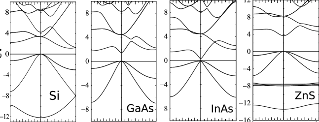
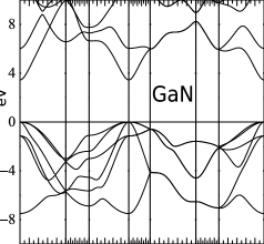
Figure 1: Energy bands calculated by the QSGW$\alpha$ method (Eq. (9)), with $\alpha$ chosen to reproduce the experimental band gap $E_{G}$. In wurtzite GaN, $E_{G}$=3.44eV O.Madelung (1996), and $\alpha=0.79$. Data for other compounds can be found in Table 1.

Table 1: Eigenvalues of semiconductors relative to the valence band maximum at $\Gamma$. The QS$GW$ column depict results without spin-orbit coupling; values in parentheses include spin-orbit coupling. Column QS$GW\alpha$ shows values after scaling defined in Eq. (9). $\alpha$ is chosen so that the QS$GW\alpha$ potential (without spin-orbit coupling) reproduces the experimental minimum band gap at room temperature.

Si	Expt.	QS$GW$	QS$GW\alpha$
			$\alpha=0.85$
$\Gamma_{15c}$	3.34	3.45(3.41)	3.32
$L_{6c}$	2.04	2.35	2.21
$E_{g}$	1.12	1.23(1.11)	1.12
$\Gamma_{2^{\prime}c}$	4.15	4.38	4.21
GaAs	Expt.	QS$GW$	QS$GW\alpha$
			$\alpha=0.68$
$\Gamma_{6c}$	1.42	1.93(1.81)	1.42
$L_{6c}$	1.66	2.11	1.72
$X_{6c}$	1.97	2.12	1.90
$\Gamma_{7c}$	4.50	4.74	4.42
InAs	empPP	QS$GW$	QS$GW\alpha$
			$\alpha=0.65$
$\Gamma_{6c}$	0.37	0.79(0.68)	0.38
$L_{6c}$	1.53	1.86	1.51
$X_{6c}$	2.28	2.10	1.90
$\Gamma_{7c}$	4.39	4.84	4.51
ZnS	Expt.	QS$GW$	QS$GW\alpha$
			$\alpha=0.83$
$\Gamma_{6c}$	3.68	4.04(4.01)	3.68
$L_{6c}$		5.45	5.05
$X_{6c}$		5.05	4.74
$\Gamma_{7c}$		8.67	8.26

Here we treat Si, GaAs, InAs, zincblende ZnS, and wurtzite GaN. For each material we calculate a self-consistent noninteracting hamiltonian $H^{0}$ through the QSGW formalism. Spin-orbit coupling is neglected, following prior work Sano and Yoshii (1995); Jung et al. (1996). Table 1 shows calculated values at high-symmetry points, compared with available experimental data. As we and others have notedKotani et al. (2007a); van Schilfgaarde et al. (2006a); Shishkin et al. (2007), the QSGW gap is systematically overestimated because the RPA underestimates the screening. (Also the GaAs calculation used a smaller basis what was reported in van Schilfgaarde et al. (2006a), resulting in an additional overestimate of $\sim$0.05 eV.) To compare the QSGW results to experiment, we must take into account other contributions: spin-orbit coupling, zero-point motionCardona and Thewalt (2005), and finite temperature all reduce the gap slightlyvan Schilfgaarde et al. (2006b).

To obtain the most reliable IIR, we slightly modify $H^{0}$ to reproduce the experimental gap at room temperature without including these contributions explicitly. To do this, we add an empirical scaling (“QSGW$\alpha$” correction) following the procedure used in Ref.Chantis et al. (2006). We scale the one-body Hamiltonian as follows:

$$H^{\alpha}=H^{0}+(1-\alpha)(\widetilde{\Sigma}-V_{\rm xc}^{\rm LDA})$$ (9)

where $\widetilde{\Sigma}$ is the static version of the self-energy (see Eq.(10) in Ref.Kotani et al. (2007a)). Table 1 shows numerical values both with and without the scaling. As we showed in Ref.Chantis et al. (2006), effective masses are also well reproduced. Thus we can set up a satisfactory $H^{\alpha}$ with a single parameter $\alpha$. This procedure is reasonable because the uncorrected gaps are already close to experiment and $1-\alpha$ is not large. The materials-dependence of $\alpha$ shown in Table 1 originates largely from the dependence of SO coupling and finite temperature on material. If these were taken into account by improving $H^{0}$ explicitly, a universal choice of $\alpha\sim 0.8$ would reproduce the experimental gaps in the Table to within $\sim$0.1eV. (Alternatively, adopting the present procedure with a universal $\alpha\sim 0.75$ accomplishes much the same thing.) Table 1 shows that the experimental energy dispersions are also well reproduced where they are well known (Si and GaAs). This systematic tendency is found for many other materials, including ZnO, Cu₂O, NiO and MnO Faleev et al. (2004); Kotani et al. (2007a), and GdNChantis et al. (2007). It implies that the QSGW$\alpha$ procedure is broadly applicable with comparable accuracy to many environments, e.g, to InAs/GaAs grain boundaries. The QSGW$\alpha$ energy bands are shown in Fig.1.

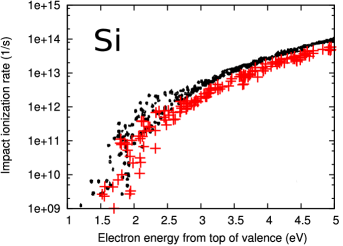
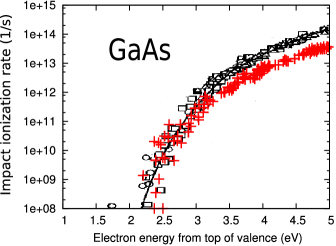
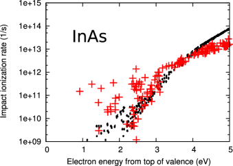
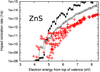
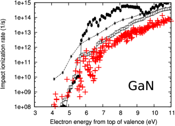
Figure 2: (color online) Impact ionization rates $\tau_{{\bf k}n}^{-1}$ as a function of the initial electron energy $\varepsilon_{\rm in}$ (measured from the bottom of conduction band). The present $GW$A calculation is shown by large (red) plus signs. It is superposed on previous calculations: Si and InAs from Sano and Yoshii Sano and Yoshii (1995), GaAs from Jung et al. Jung et al. (1996), ZnS and GaN from Kuligk et al. Kuligk et al. (2005). Open boxes in the ZnS and GaN data are EPP results from Picozzi et al. Picozzi et al. (2002b); solid circles are exact exchange results Kuligk et al. (2005). We used 500 ${\bf k}$ points in the 1st Brillouin zone for GaN, and 1728 points for the cubic compounds (regular mesh including the $\Gamma$ pointKotani et al. (2007a)). Owing to the limited number of ${\bf k}$ points, there are some numerical errors, e.g. a factor of order 2 when IIR $\lesssim$ 1e+10). The error is not large enough to affect our conclusions.

Given $H^{\alpha}$, we perform a one-shot $GW$A calculation using the method detailed in Ref.Kotani et al. (2007a), and calculate $\tau_{{\bf k}n}^{-1}$ from Eq. (1). To reduce the computational time we truncate the product basis for each atomic site to $l\leq{}1$. This limits the degrees of freedom for the local-field correction in the dielectric function. However, we checked that this little affects the results. To obtain $Z_{{\bf k}n}$ in Eq. (1), we need to calculate the derivative of the self-energy $\frac{\partial{\rm Re}\Sigma(\omega)}{\partial\omega}$ at $\varepsilon_{{\bf k}n}$, though $Z$ contributes a relatively unimportant factor $\sim 0.8$. The main computational cost of the IIR calculation comes from the sum of the pole weights on the real axis; see Eq. (58) in Ref.Kotani et al. (2007a). This corresponds to the convolution of Im$G$ and Im$W$, Eq. (2), after Im$W$ is obtained from integration by the tetrahedron method Kotani et al. (2007a). Fig.2 shows our results for $\tau_{{\bf k}n}^{-1}$. The $x$-axis denotes the initial electron energy $\varepsilon_{\rm in}$ measured from the bottom of the conduction band; $\varepsilon_{\rm in}>E_{G}$ is a hard threshold below which IIR is zero. The present results, depicted by large plus signs, are superposed on results taken from previous work.

The IIR has a typical feature as already shown in Fig.1 in Ref.Sano and Yoshii (1994), that is, the IIR as function of $\varepsilon_{\rm in}$ are widely scattered at low $\varepsilon_{\rm in}$ because of the limited number of transitions that conserve energy and momentum. The scatter diminishes at high energy because of an averaging effect which smears the anisotropy in the Brillouin zone as discussed in Sano and Yoshii (1994). Our results for Si and GaAs correspond rather well to previous work. Details for the IIR are already well analyzed Sano and Yoshii (1992, 1994, 1995); Jung et al. (1996); Kuligk et al. (2005); Picozzi et al. (2002b, a).

Turning to ZnS and GaN, we superpose our results on those presented by Kuligk et al. in Figs. 9 and 10 of Ref.Kuligk et al. (2005), which include exact exchange (EXX) (solid symbols) and EPP results from Ref.Picozzi et al. (2002b) (open symbols). The EPP and the present calculations appear mostly similar apart from an approximately constant factor; however the EXX results show rather different behavior, particularly in GaN. This is likely because the EPP and QSGW$\alpha$ energy bands are quite similar to each other, but they are quite different from the EXX case (see Figs 2 and 3 in Ref.Kuligk et al. (2005)).

A large discrepancy with EPP is seen only in InAs. Our data is superposed on the calculations by Sano and Yoshii Sano and Yoshii (1995). We obtain high IIR at low initial electron energies $\varepsilon_{\rm in}\gtrsim$1 eV. Such high IIR comes from initial electrons near the conduction band minimum at the $\Gamma$ point. Since the band gap and effective mass are small in InAs, there are states not far from $\Gamma$ with energy $\varepsilon_{\rm in}>E_{G}$, which can generate an electron-hole pair. This occurs only for InAs in the cases studied, but generally occurs for narrow gap semiconductors. For the discrepancy with results of Sano and Yoshii may be due to their constant matrix elements approximation, which is not suitable for such a narrow gap material (see Ref.Sano and Yoshii (1995) near Eq.(2)).

In conclusion, we have calculated the IIR for several materials in the $GW$A, after a theoretical discussion of its application to the IIR. In principle, the method presented here will be applicable even to inhomogeneous systems such grain boundaries and quantum dots where we expect very strong IIR. The present calculations correspond reasonably well to prior work, with the exception of the narrow gap material InAs. High IIR would be expected universally in similar narrow gap materials such as GaSb, InSb, and InN. This indicates that careful consideration for the IIR might be required when we use such materials for devices.

This work was supported by ONR contract N00014-7-1-0479, and the NSF QMHP-0802216. We are also indebted to the Ira A. Fulton High Performance Computing Initiative.

References

- D.K.Ferry (2000) D.K.Ferry, Semiconductor Transport (Taylor & Francis, London, 2000).
- Schaller and Klimov (2004) R. Schaller and V. Klimov, Phys. Rev. Lett. 92, 186601 (2004).
- Kane (1967) E. O. Kane, Phys. Rev. 159, 624 (1967).
- Sano and Yoshii (1992) N. Sano and A. Yoshii, Phys. Rev. B 45, 4171 (1992).
- Sano and Yoshii (1994) N. Sano and A. Yoshii, Journal of Applied Physics 75, 5102 (1994), URL http://link.aip.org/link/?JAP/75/5102/1.
- Sano and Yoshii (1995) N. Sano and A. Yoshii, Journal of Applied Physics 77, 2020 (1995), URL http://link.aip.org/link/?JAP/77/2020/1.
- Jung et al. (1996) H. K. Jung, K. Taniguchi, and C. Hamaguchi, Journal of Applied Physics 79, 2473 (1996).
- Seidl et al. (1996) A. Seidl, A. Göring, P. Vogl, J. A. Majewski, and M. Levy, Phys. Rev. B 53, 3764 (1996).
- Picozzi et al. (2002a) S. Picozzi, R. Asahi, C. Geller, A. Continenza, and A. J. Freeman, Phys. Rev. B 65, 113206 (2002a).
- Picozzi et al. (2002b) S. Picozzi, R. Asahi, C. B. Geller, and A. J. Freeman, Phys. Rev. Lett. 89, 197601 (2002b).
- Kotani (1994) T. Kotani, Phys. Rev. B 50, 14816 (1994), phys. Rev. B51 13903(E).
- Städele et al. (1997) M. Städele, J. A. Majewski, P. Vogl, and A. Görling, Phys. Rev. Lett. 79, 2089 (1997).
- Kuligk et al. (2005) A. Kuligk, N. Fitzer, and R. Redmer, Physical Review B (Condensed Matter and Materials Physics) 71, 085201 (pages 6) (2005), URL http://link.aps.org/abstract/PRB/v71/e085201.
- Faleev et al. (2004) S. V. Faleev, M. van Schilfgaarde, and T. Kotani, Phys. Rev. Lett. 93, 126406 (2004).
- van Schilfgaarde et al. (2006a) M. van Schilfgaarde, T. Kotani, and S. Faleev, Phys. Rev. Lett. 96, 226402 (2006a).
- Kotani et al. (2007a) T. Kotani, M. van Schilfgaarde, and S. V. Faleev, Physical Review B 76, 165106 (pages 24) (2007a).
- Kotani et al. (2007b) T. Kotani, M. van Schilfgaarde, S. V. Faleev, and A. Chantis, Journal of Physics: Condensed Matter 19, 365236 (8pp) (2007b).
- Chantis et al. (2007) A. N. Chantis, M. van Schilfgaarde, and T. Kotani, Physical Review B 76, 165126 (2007).
- Chantis et al. (2006) A. N. Chantis, M. van Schilfgaarde, and T. Kotani, Phys. Rev. Lett. 96, 086405 (2006).
- Echenique et al. (2000) P. Echenique, J. Pitarke, E. Chulkov, and A. Rubio, CHEMICAL PHYSICS 251, 1 (2000).
- O.Madelung (1996) O.Madelung, Semiconductors - Basic data 2nd Ed. (Springer, 1996).
- Shishkin et al. (2007) M. Shishkin, M. Marsman, and G. Kresse, Physical Review Letters 99, 246403 (2007).
- Cardona and Thewalt (2005) M. Cardona and M. L. W. Thewalt, Rev. Mod. Phys. 77, 1173 (2005).
- van Schilfgaarde et al. (2006b) M. van Schilfgaarde, T. Kotani, and S. V. Faleev, Phys. Rev. B 74, 245125 (2006b).