Charged particle-display

Abstract

An optical shutter based on charged particles is presented. The output light intensity of the proposed device has an intrinsic dependence on the interparticle spacing between charged particles, which can be controlled by varying voltages applied to the control electrodes. The interparticle spacing between charged particles can be varied continuously and this opens up the possibility of particle based displays with continuous grayscale.

I Introduction

The flexibility and bistability are the two key points in the next generation display technologies. The flexibility implies the display would be thin, lightweight, and ultimately, paper like, meaning it would be cheap enough to be disposable. The bistability implies the technology would be ecologically friendly. In the bistable display, the image does not need to be refreshed until rewritten and, therefore, a low level of power consumption is expected for still images. Unfortunately, for motion pictures, the bistability has no advantages in power savings over nonbistable technologies such as liquid crystal displays (LCDs), plasma display panels (PDPs), and displays based on organic light emitting diodes commonly referred to as OLEDs.

The display technologies based on particles are the most prominent candidates for a flexible and bistable displays. The earliest display based on particles dates back to 1970’s when OtaOta filed for a patent. Since then various particle-displays based on electrophoresis and electrowetting principles have emerged to form what is now referred to as “E-paper technologies” in the industry.twisting_ball ; Mizuno ; Matsuda ; Jacobson ; Ding In electrophoresis, particles are usually suspended in a fluid. Because the speed at which particles move inversely vary with fluid density, particle-displays based on electrophoresis have slow response time, typically on the order of $300\,\textnormal{ms}.$nature ; Whiteside ; T. Kosc This makes motion pictures unsuitable for electrophoretic particle-displays. The issue of slow response time in electrophoretic particle-displays, however, has been resolved with the unveil of Quick Response Liquid Powder Display (QR-LPD) by Hattori et al.QR_LPD1 ; QR-LPD2 ; QR-LPD3 ; QR_LPD4 The QR-LPD is distinguished from the rest of particle based displays in that it uses air as the particle carrying medium rather than fluid. Because the particles in QR-LPD move in air, its response time is at $0.2\,\textnormal{{ms},}$ which is even faster than LCDs. The submillisecond response time makes QR-LPD the only candidate based on particle-display capable of handling motion pictures, and researches are being conducted for particle-displays with air as the particle carrying medium.LG2

Common to all particle-displays, regardless of whether air or fluid is used as the particle carrying medium, is the lack of continuous grayscale. Here, the terminology, “continuous grayscale,” is referred to as the number of grayscale levels required to produce desired number of colors. In principle, a display device with continuous grayscale can generate an infinite range of colors. That being clarified, a high grayscale range is essential to quality displays. Without it, the images displayed on monitors would be dull.Stephen_Johnson Recently, it has been reported particle-display based on QR-LPD can generate up to 16 grayscale levels (i.e., 4 bits), which corresponds to the capability of generating 4096 colors.QR-LPD-16gray-level ; QR-LPD-16gray-level-2 To the proponents of other competing flat panel display technologies, such as flexible LCDs, PDPs, or OLEDs, 4 bits of gray scale range could hardly be considered a technological milestone. However, considering only 4 grayscale levels were possible just a few years ago for particle-displays, 16 grayscale levels is a significant technological advancement for the E-paper technology.QR-LPD-4gray-level

The most well known E-paper technology, E-Ink, obtains different gray states through modulation of voltages supplied to the control electrodes. The same mechanism is employed by particle-displays based on QR-LPD for achieving different gray states.T. Kosc ; QR-LPD-4gray-level Because the voltage is modulated at a value lower than the saturation voltage, which is the voltage required to display either all black or all white for a simple black-and-white display, the displayed image would have intensity somewhere between that of completely black and completely white. This approach to achieve different gray states, however, is done at the cost of losing bistability. Since the pixel is being constantly modulated to sustain a gray state, the situation is equivalent to motion pictures and the power savings from bistability no longer applies to gray states. In spite of the lost bistability advantages over the other competing flexible display technologies, the speed at which particle can be modulated is limited by its finite inertia (mass) and this places a practical limit on the extent to which the grayscale levels of particle-display can be enhanced by the aforementioned method. Most recently, ChimQR-LPD-64gray-level demonstrated a 64 grayscale levels (or 6bits) for particle-display based on QR-LPD for his masters thesis project at Delft University of Technology. However, to generate 64 grayscale levels, the DATA Driver, which is a serial to parallel shift register that shifts data words of 6 bits per clock cycle, is required.

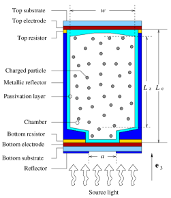
Figure 1: (Color online) Transflective display based on charged particles.

In this work, a display architecture based on charged particles is presented. Unlike the previous particle-display technologies, the proposed device has potential to generate continuous grayscale levels without sacrificing the benefit of bistability. Also, the proposed particle-display technology, in principle, does not require complicated voltage modulation schemes to generate different gray states.SNCHO

II Charged particle-display

II.1 Device structure

The cross-sectional schematic of an optical shutter based on charged particles of same polarity is illustrated in Fig. 1. In the figure, the two electrodes, where each is labeled top and bottom electrodes, constitute the control electrodes. Because the light must be transmitted through the control electrodes, the electrodes are chosen from optically transparent conductors. The chamber, wherein the particles reside, can be a vacuum, filled with noble gas, or filled with air. The metallic reflectors, which forms the lateral surface of the chamber, are electrically connected to one of the control electrodes. This make metallic reflectors not only to reflect light, but also function as to keep particles from aggregating to the lateral surface of chamber. The optically transparent passivation layer, which is treated on the inner surface of the chamber, functions to prevent charge transfer between particles and conductors. For positively charged particles inside the chamber, the hydrophobic treatment on the surface of the passivation layer, which is not explicitly shown in the figure, for example, prevents particles from sticking to the surface.

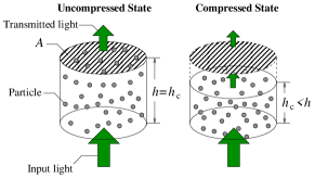
Figure 2: (Color online) Transmission of light through a medium filled with total of $N$ suspended spherical particles. Both of the compressed and the uncompressed cases are shown.

II.2 Operation principle

The intensity of light transmitted through a medium filled with suspended spherical particles, illustrated in Fig. 2, is given by

$$I=I_{0}\exp\left[-\frac{36n\pi kfh}{\lambda\left(n^{2}+2\right)^{2}}\right],$$ (1)

where $n$ and $k$ are, respectively, the real and the imaginary part of the complex refractive index for the medium and the particles suspended in it; $I_{0}$ is the initial intensity, $\lambda$ is the wavelength of incidence light, $h$ is the height (or thickness) of the volume containing charged particles, and $f$ is the volume fraction of particles.Bohren_Huffman In explicit form, the volume fraction of particles is

$$f=\frac{Nv_{\textup{p}}}{Ah_{\textup{c}}},$$

where $N$ is the total number of particles in the optical chamber, $v_{\textup{p}}$ is the volume of a single particle, $h_{\textup{c}}$ is the height of compressed cylinder containing charged particles, and $A$ is the cross-sectional area of the cylindrical chamber illustrated in Fig. 2. Throughout this work, I shall refer to terms such as “compressed state” or “compressed particle volume” to denote the compression of the volume containing particles. Insertion of $f$ into Eq. (1) gives

$$I=I_{0}\exp\left(-\frac{C}{h_{\textup{c}}}\right), C=\frac{36n\pi khNv_{\textup{p}}}{\lambda\left(n^{2}+2\right)^{2}A},$$ (2)

where $C$ is just a constant.

The complex dielectric constant, $\tilde{\varepsilon},$ and the complex refractive index, $\tilde{n},$ are expressed in form as

$$\tilde{\varepsilon}=\varepsilon_{1}+i\varepsilon_{2}, \tilde{n}=n+ik,$$ (3)

where $\varepsilon_{1}$ and $n$ are the real parts, and $\varepsilon_{2}$ and $k$ are the imaginary parts. For the complex refractive index, $n$ represents the real refractive index and $k$ is the extinction coefficient (or the absorption coefficient). The two, $\tilde{\varepsilon}$ and $\tilde{n},$ are related by the expression

$$\tilde{\varepsilon}-\tilde{n}^{2} =0.$$

With the real and imaginary parts inserted for $\tilde{\varepsilon}$ and $\tilde{n}$ from Eq. (3), I have

$$\varepsilon_{1}+i\varepsilon_{2}-\left(n+ik\right)^{2} =0.$$

The resulting expression can be rearranged to yield

$$\left(\varepsilon_{1}-n^{2}+k^{2}\right)+i\left(\varepsilon_{2}-2nk\right) =0.$$ (4)

Equation (4) can only be true if and only if the real and the imaginary parts are equal to zero independently. This requirement yields the two expressions connecting $\left(\varepsilon_{1},\varepsilon_{2}\right)$ to the optical constants $\left(n,k\right);$ and, the two expressions are

$$\varepsilon_{1}=n^{2}-k^{2}, \varepsilon_{2}=2nk.$$ (5)

Stoller et al.gold-particle-quantum measured the complex dielectric constant, $\tilde{\varepsilon}\left(\varepsilon_{1},\varepsilon_{2}\right),$ for the single gold nanoparticle. For the gold nanoparticles of diameters $10$ and $15\,\textup{nm},$ assuming a spherical morphology, they observed a reasonably good correspondence existing between complex dielectric constants of the bulk gold and the gold nanoparticles for the wavelength range of roughly $510$ to $580\,\textup{nm}.$ Their finding is of significant importance, as it allows the bulk gold dielectric constants, which is readily available, to be used for the gold nanoparticles, which is not so readily available. Since the real and the imaginary parts of the complex dielectric constant are related to the optical constants $\left(n,k\right)$ thru Eq. (5), the $n$ and $k$ for the gold nanoparticles are readily available once $\varepsilon_{1}$ and $\varepsilon_{2}$ are known from the bulk counterpart. The vice versa is also true, of course. Fortunately, Johnson and Christy measured the optical constants for the bulk copper, silver, and the bulk gold.gold-bulk Justified by the findings of Stoller et al.,gold-particle-quantum for $\lambda=550\,\textup{nm},$ assuming the gold nanoparticle of radius $r_{\textup{p}}=7.5\,\textup{nm},$ the $n$ and $k$ measurements from the work of Johnson and Christy,gold-bulk

$$\textup{bulk gold:}\;\tilde{n}=n+ik, \left\{\begin{array}[]{c}n=0.43,\\ k=2.455,\\ \lambda=550\,\textup{nm},\end{array}\right.$$ (9)

can be utilized for the gold nanoparticles to plot Eq. (2) for the transmitted intensity.

For a spherical gold nanoparticle, the particle volume, $v_{\textup{p}},$ is given by

$$v_{\textup{p}} =\frac{4}{3}\pi r_{\textup{p}}^{3},$$

where $r_{\textup{p}}$ is the particle radius. Assuming the diameter of $15\,\textup{nm}$ for the gold nanoparticle, $v_{\textup{p}}$ becomes

$$r_{\textup{p}}=7.5\,\textup{nm}, v_{\textup{p}}=1.77\times 10^{-24}\,\textup{m}^{3}.$$ (10)

To plot Eq. (2), I shall assume the following values for the chamber parameters, (the height $h$ and the cross-sectional area $A$), and the particle number, $N,$

$$\left\{\begin{array}[]{c}h=100\,\mu\textup{m}=1\times 10^{-4}\,\textup{m},\\ A=\pi h^{2}=3.14\times 10^{-8}\,\textup{m}^{2},\\ N=2.46\times 10^{8}.\end{array}\right.$$ (11)

Figure 3: Schematic of curves illustrating the intensity, $I,$ of transmitted light as a function of compression height, $h_{\textup{c}}.$

Before going ahead with plotting Eq. (2), it is worthwhile to double check if the total number of particles, $N,$ specified in Eq. (11) is reasonable. With chamber parameters as defined in Eq. (11), the volume of the cylindrical chamber is

$$V=Ah=\pi h^{3}.$$

Suppose the charged spherical particles can be compressed and enclosed in a confined volume in such a way that neighboring particles actually touch each other. How many particles, under such restrictions, can be fitted inside the chamber defined by Eq. (11)? The answer is $N_{\textup{max}}$ and its expression is

$$N_{\textup{max}}=\frac{V}{v_{\textup{p}}}=\frac{3}{4}\left(\frac{h}{r_{\textup{p}}}\right)^{3}.$$ (12)

For the spherical particle of radius $r_{\textup{p}}=7.5\,\textup{nm},$ the $N_{\textup{max}}$ is roughly

$$N_{\textup{max}}\approx 1.7\times 10^{12}.$$ (13)

For the charged particles, the condition of neighboring particles actually touching each other is not possible due to Coulomb repulsion, unless the external compression force is infinite. Nonetheless, the expression for $N_{\textup{max}},$ defined in Eq. (12), provides the upper limit for $N$ inside the chamber.

The physical optical shutter based on charged particles must be compressible in order to allow variations in transmission intensity, which imposes the condition,

$$N<N_{\textup{max}}.$$

Equivalently, the variability of transmission intensity thru compression requires $N\neq 0$ and this further modifies the condition for $N$ as

$$0<N<N_{\textup{max}}.$$ (14)

The inequality condition for $N,$ defined in Eq. (14), can be understood from the illustration shown in Fig. 3, where some of the possible curves for the transmission intensity, $I,$ as a function of the compression height, $h_{\textup{c}},$ are shown. The cases where $N=0$ and $N=N_{\textup{max}}$ are represented by the curves corresponding to $\triangle I/\triangle h_{\textup{c}}=0$ at $I=I_{0}$ and $I=0,$ respectively. Similarly, the the curve corresponding to $\triangle I/\triangle h_{\textup{c}}=0$ at $I=0$ in the figure represents the case where $N=N_{\textup{max}}.$ For $N=N_{\textup{max}},$ the particles in the chamber are already maximally compressed and, therefore, no light gets transmitted. On the other hand, for $N=0,$ all light gets transmitted through the optical shutter, as the inside of the optical shutter is a void.

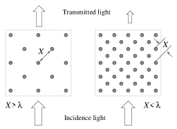
Figure 4: Array of metallic nanoparticles in grid formation. The parameter $X$ is the grid (or particle-particle) spacing and $\lambda$ is the wavelength of the incidence light. For the charged particles inside the chamber, the parameter $X$ can only be thought of as the time averaged mean particle-particle distance between the nearest neighboring particles. Nonetheless, the grid representation illustrated here serves the purpose of initiating the crude connection between the wavelength of incidence light, $\lambda,$ and the total particle number, $N.$

For the case of any finite $N$ satisfying the condition defined in Eq. (14), the curve for the transmission intensity must necessarily lie in the region between the two extreme cases, $N=0$ and $N=N_{\textup{max}},$ as schematically demonstrated in Fig. 3. Three such curves, corresponding to finite $N,$ are illustrated in the figure: (1) the upper curve represented by $\triangle I/\triangle h_{\textup{c}}=f\left(h_{\textup{c}}\right),$ (2) the curve represented by $\triangle I/\triangle h_{\textup{c}}=\alpha,$ and (3) the lower curve represented by $\triangle I/\triangle h_{\textup{c}}=f\left(h_{\textup{c}}\right),$ where $\alpha$ is a constant and $f\left(h_{\textup{c}}\right)$ is a function of $h_{\textup{c}}.$ The two curves corresponding to $\triangle I/\triangle h_{\textup{c}}=f\left(h_{\textup{c}}\right)$ only appreciably varies in transmission intensity with compression within the window of $\beta-\delta,$ where $\beta-\delta\ll h.$ Such curves are associated with $N,$ in which the $N$ is finite but close to either $N=0$ or $N=N_{\textup{max}}.$ Because the transmission intensity only appreciably varies within $\beta-\delta\ll h$ for such choices of $N,$ the gray states are difficult to achieve as it requires very precise control of the compression height. For example, assuming the particles can be compressed at the increment in $\triangle h_{\textup{c}},$ the fact that $\beta-\delta\approx\triangle h_{\textup{c}}$ makes it difficult to achieve gray states. To achieve gray states, the $\triangle h_{\textup{c}},$ which defines the sensitivity of compression, must be much smaller than $\beta-\delta.$ Consequently, the transmission intensity curves for the aforementioned choices of $N$ are only good for displaying either completely bright or completely dark transmission states.

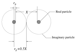
Figure 5: The nanoparticles of radius $r_{\textup{p}}$ are separated by $X,$ which is the nearest surface to surface separation between two neighboring particles. The imaginary particles of radius $r_{\textup{I}}=r_{\textup{p}}+0.5X$ are, however, in closed packed formation for a given nearest surface to surface separation of $X.$

The optimal design for the presented optical shutter is achieved by choosing $N$ for the total particle number in the chamber in such way that the curve for the transmission intensity goes like $\triangle I/\triangle h_{\textup{c}}=\alpha,$ where $\alpha$ is a constant, in Fig. 3. Because the curve is linear for the transmission intensity, the window of range in which compression can be done is maximized, $h-\delta\lesssim h.$ For this particular choice of $N,$ the $\triangle h_{\textup{c}},$ which is the increment at which particles can be compressed, is much less than $h-\delta,$ i.e., $h-\delta\gg\triangle h_{\textup{c}},$ and the number of different gray states that can be achieved is given by

$$N_{\textup{gray}} =\frac{h-\delta}{\triangle h_{\textup{c}}}.$$ (15)

In principle, the $\triangle h_{\textup{c}}$ can be made finer and finer as desired. In reality, the fineness of $\triangle h_{\textup{c}}$ is limited by the system design. Nevertheless, with the right choice of $N,$ the grayscale levels in number of $N_{\textup{gray}},$ as defined in Eq. (15), is possible with the presented optical shutter based on charged particles. The question remains to be answered is this: how do we go about obtaining the right $N$? To answer this, I shall refer to the illustration shown in Fig. 4.

Due to the wave nature of light, the total particle number and the transmission intensity depend on the wavelength, $\lambda,$ of the incidence light. As a rudimentary assumption, the transmission loss of an electromagnetic wave passing through an array of metallic particles decreases for $X\gg\lambda$ and increases for $X\lesssim\lambda/j,$ where $j=2,\,3,\,\cdots,$ which is schematically illustrated in Fig. 4. The case where $X\gg\lambda$ represents the situation in which $N$ is very small, whereas the case where $X\lesssim\lambda/j,$ represents the situation in which $0\ll N\ll N_{\textup{max}},$ provided the $j$ is not too large. It is, therefore, not too bad to impose the condition, $X\approx\lambda/2,$ for $X$ in estimating for the total number of particles in the chamber. For $\lambda=550\,\textup{nm},$ this condition for $X$ yields the value of $X=275\,\textup{nm}.$ To figure out exactly how man particles can be fitted inside the chamber under restriction $X\approx\lambda/2,$ the Fig. 5 is referred to. Since $X$ is the closest distance between surfaces of two nearest neighbor particles, I shall visualize an imaginary particle of radius $r_{\textup{I}},$

$$r_{\textup{I}} =r_{\textup{p}}+0.5X.$$ (16)

Assuming the imaginary particles are close-packed inside the chamber, the problem becomes identical to the previous case, which resulted in Eq. (12). With $r_{\textup{I}}$ of Eq. (16) inserted for $r_{\textup{p}}$ in Eq. (12), the expression becomes

$$N_{\textup{min}}=\frac{3}{4}\left(\frac{h}{r_{\textup{p}}+0.5X}\right)^{3}, X=\frac{\lambda}{2},$$ (17)

where $N_{\textup{max}}$ has been replaced by $N_{\textup{min}}.$ With $N_{\textup{min}}$ defined in Eq. (17), the number of particles inside the chamber may be chosen according to the inequality,

$$0\ll N_{\textup{min}}\lesssim N\ll N_{\textup{max}}.$$ (18)

It can be easily verified that $N_{\textup{min}}\gg 0.$ For $X=275\,\textup{nm},$ which corresponds to the half wavelength of $\lambda=550\,\textup{nm},$ $N_{\textup{min}}$ is roughly $N_{\textup{min}}\approx 2.46\times 10^{8}.$ This value for $N_{\textup{min}}$ is much larger than zero, but it is much smaller than $N_{\textup{max}},$ which has the value $N_{\textup{max}}\approx 1.7\times 10^{12}$ from Eq. (13). For the optical shutter involving charged particles of spherical morphology and the cylindrical chamber of specifications defined in Eq. (11), the inequality condition for $N,$ Eq. (18), becomes

$$\frac{3}{4}\left(\frac{h}{r_{\textup{p}}+\frac{\lambda}{2n}}\right)^{3}\lesssim N\ll\frac{3}{4}\left(\frac{h}{r_{\textup{p}}}\right)^{3}, n=2,3,\cdots.$$ (19)

Equation (2) has been computed using gold nanoparticles as the charged particles (the gold nanoparticle was chosen only because its optical constant data, $n$ and $k,$ were readily available). For the charged particles and the incidence light, the parameters defined in Eq. (9) were used. The parameters defined in Eq. (11) were used for the chamber specification. Using Eq. (2), the transmission intensity for different values of $N$ were considered and the results are shown in Fig. 6. The $N=30\times 10^{6}$ curve is the case where particle number is relatively low in the chamber. As it can be observed, for low particle numbers in the chamber, the intensity does not vary well with compression except for small $h_{\textup{c}},$ which is consistent with the curve represented by $\triangle I/\triangle h_{\textup{c}}=f\left(h_{\textup{c}}\right)$ in Fig. 3. Contrarily, the $N=900\times 10^{6}$ curve corresponds to the case where too many particles are inside the chamber. Although the transmission intensity varies linearly with compression, which is a good characteristic of an optical shutter, the output intensity is far too low even for the brightest state. For $N=900$$\times 10^{6},$ the brightest state only transmits $10\%$ of the initial input intensity, i.e., $I/I_{0}=0.1.$ As expected, the $N=246$$\times 10^{6}$ curve in Fig. 6, which corresponds to the case where $X=\lambda/2$ for $\lambda=500\,\textup{nm},$ most resembles the curve represented by $\triangle I/\triangle h_{\textup{c}}=\alpha$ in Fig. 3. However, the brightest output intensity is only $\sim 50\%$ of the input intensity of the incidence light. Compared to LCDs, where only $\sim 5\%$ of the intensity of the incidence light from back light unit gets transmitted, the output intensity of $\sim 50\%$ is already $10$ times more efficient than LCDs.

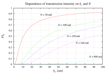
Figure 6: (Color online) Transmission intensity as a function of particle number, $N,$ and the compression height, $h_{\textup{c}}.$ The abbreviation “mil” in the figure denotes a million, i.e., $1\times 10^{6}.$

The same principle, which is inherent in Eq. (2), applies to the proposed optical shutter, Fig. 1. In the presented device, the chamber is filled with charged particles of same polarity and this can be identified with the medium filled with suspended particle in Fig. 2. The on set of electric field inside the chamber, which is done by controlling the voltage over one of the electrodes, causes particles to be compressed in volume, as illustrated in Fig. 7. Since the particles are assumed to be positively charged, they are compressed in the direction of electric field. Eventually, the compression comes to a stop when particle-particle Coulomb repulsion counterbalances the compression induced by the control electrodes.

In principle, the level of compression for the particle volume can be varied continuously. Because the intensity of transmitted light varies with compression, i.e., Eq. (2), the display based on charged particles has the potential to generate continuous gray levels. Also, since the control electrodes form a capacitor, provided there is no leakage (or negligible) current across the capacitor, the electric field inside the chamber can be sustained even when the device is disconnected from power. This opens up the possibility of a bistable mode for gray states as well.

The presented device works as an optical shutter, provided the charged particles can be effectively prevented from piling up at the surface of dielectric walls. When a charged particle is brought close to the dielectric surface, the bound charges within the dielectric get redistributed in order to reduce the field originating from the charged particle placed near vicinity of dielectric surface. Such is illustrated in Fig. 8. For the case where a positively charged particle is placed near the surface of a dielectric, the surface bound charges of opposite polarity get induced and distributed near the inner surface of dielectric. As a result, the positively charged external particle gets pulled to the dielectric surface and, eventually, sticking to the surface of dielectric, which process is illustrated in Fig. 9. If there are more than one positively charged particles placed at the vicinity of dielectric surface, the aforementioned process continues and, eventually, layers get formed, for example, the layers $A$ and $B$ in the figure. This process does not continue indefinitely, however, as the bound charges of opposite polarity within the dielectric get eventually shielded by the positively charged particles forming layers over the dielectric surface. Because the particles in each layer are charged with same polarity, the Coulomb repulsion keeps the two particles from touching each other. Assuming the layer $B$ is sufficient to shield completely the negatively charged surface bound charges within the dielectric, the remaining positively charged particles in the region between two dielectric walls would have no other places to go, except to continuously bounce back and forth within the region, which region has been indicated by $M$ in Fig. 9.

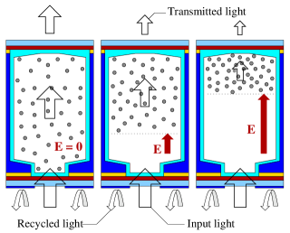
Figure 7: (Color online) The on set of electric field compresses the filled volume for charged particles.

The aforementioned description for an optical shutter, however, has a serious problem which is associated with the particle layers forming on the surface of dielectric walls. Assuming the path of light propagation is along the horizontal axis, the light enters the device from the left and exits at the right or vice versa. In principle, the compression of charged particles in region, $M,$ controls the intensity of transmitted light. The problem arises because the charged particles forming layers $A$ and $B$ on the surface of dielectric walls may no longer be optically transparent. As previously discussed, using the illustration in Fig. 4 as an example, metallic particles in an array of grid formation severely reduces the intensity of transmitted light for grid spacing, $X,$ much less than the wavelength, $\lambda,$ of the incidence light. I now discuss the ways to resolve this complication.

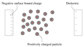
Figure 8: (Color online) Charged particles near dielectric wall.

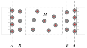
Figure 9: (Color online) Charged particles in region $M$ are shielded from the negatively charged surface bound charges within the dielectric wall.

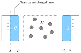
Figure 10: (Color online) Transparent charged layer formed by ISAM or electron beam irradiation method effectively plays the role of positively charged particle layers at $A$ and $B.$

It is well known that the surface of a typical $SiO_{2}$ glass becomes hydrophilic in an open air as a result of the silane group at the surface of glass combining with oxygen.hydrophilic_1 ; hydrophilic_2 This has the effect of making the surface of glass to be slightly negatively charged and any positively charged particles in vicinity would be attracted to the glass surface forming layers such as those, e.g., $A$ and $B,$ illustrated in Fig. 9. Unless the attracted, positively charged, particles are optically transparent, the device would not be able to function as an optical shutter for no light would to pass through the device. Necessarily, the role of layers $A$ and $B$ in Fig. 9 must be played out by particles of same polarity as those residing in region $M,$ but distinguished from those residing in region $M$ in that they are optically transparent. One way to achieve this is to chemically treat the surface of glass so as to make it hydrophobic. The hydrophobic treatment of glass electrically neutralizes the glass surface, thereby significantly reducing the oppositely charged particles from sticking to the glass surface. For large and weakly charged positive particles, simple electrical neutralization of glass surface by hydrophobic treatment is sufficient to keep particles from permanently sticking to the surface. In such system, charged particles are continuously bounced off of the wall and do not stick to the surface. However, for smaller and well charged positive particles, simple hydrophobic treatment of glass surface is not sufficient to prevent oppositely charged particles from sticking to the glass surface. For such cases, it is necessary to make the surface of glass net positively charged. This can be easily done by utilizing the technique known as “ionically self assembled monolayer” (ISAM), in which technique charged particles, polymers, or monomers of preferred polarity are physically attached to the surface.charged_glass_4_ISAM Alternatively, and more directly, the glass may be irradiated with electron beam to physically embed charged particles inside the glass medium.charged_glass_1 ; charged_glass_2 In this latter method, for example, net negative charges may be made to accumulate inside the glass. This has the effect of inducing positive charges on the surface of glass, which repels positive charged particles in vicinity of the glass surface, thereby preventing particles from sticking to the surface. In summary, the role of positively charged particle layers, $A$ and $B$ in Fig. 9, may be effectively get taken cared by the aforementioned ISAM or the electron beam irradiation methods; and, using these alternative techniques, the glass surface repels charged particles inside the chamber and it is optically transparent, as illustrated in Fig. 10.

To utilize charged particles in displays, a quantitative understanding of how design parameters, such as $\left(L_{\textup{e}},L_{\textup{z}},\xi\right)$ for the sub-pixel dimensions and $\left(r,\rho_{\textup{m}},Q\right)$ for the charged particle, enter into the compression mechanism is required. Here, $r$ is the particle radius (assuming a spherical particle), $\rho_{\textup{m}}$ is the particle mass density, and $Q$ is the net charge which the particle holds. Describing the compression mechanism in terms of the aforementioned design parameters is the task for the next section.

II.3 Theory

The optical shutter presented in this proposal relies on the density of particles in chamber to control the intensity of transmitted light. An analogy can be made to the driving under misty weather. When the density of water vapor suspended in the atmosphere is heavy, one is obscured in his or her viewing distance, as less light reaches the eye. Contrarily, the amount of light reaching the eye increases with a reduction in density of water vapor suspended in the atmosphere, thereby enabling the driver to see far distances.

The particles in chamber of the proposed optical shutter ranges in diameter anywhere from a few nanometers to several microns, assuming a spherical morphology. This range for the particle size, although small macroscopically, is much too large to be considered for a treatment within quantum domain, where the quantum theory must be used for a description. Therefore, the classical theory suffices for the description here. Since the charged particles in the system, as a whole, behave like a classical gas, the description is carried out in the realm of statistical physics.

To keep the topic presented here self-contained, I shall briefly summarize the kind of manipulations and approximations assumed in obtaining expressions which are considered crucial to the initial development of the analysis.

II.3.1 Maxwell-Boltzmann statistics

The charged particles in chamber can be treated as classical particles obeying the Maxwell-Boltzmann statistics.Reif The $i\textup{th}$ charged particle under influence of external forces, for example, gravitational and electric forces, assumes the energy

$$U_{i}=\frac{\mathbf{p}_{i}^{2}}{2m_{i}}+U_{\textup{ext}}+U_{\textup{int}}, \mathbf{p}_{i}=\sum_{j}p_{ij}\mathbf{e}_{j},$$

where $\mathbf{p}_{i}$ is the center of mass momentum for the $i\textup{th}$ charged particle and the term associated with it is the kinetic energy, $U_{\textup{ext}}$ is the interaction energy with external influences, and $U_{\textup{int}}$ is the energy contribution arising only if the particle is not monatomic.

In explicit form, $U_{\textup{ext}}$ can be expressed as

$$U_{\textup{ext}}= \sum_{j\neq i}^{N}\frac{k_{\textup{q}}Q_{i}Q_{j}}{\left[\left(x_{i}-x_{j}\right)^{2}+\left(y_{i}-y_{j}\right)^{2}+\left(z_{i}-z_{j}\right)^{2}\right]^{1/2}}+m_{i}gz_{i}$$

$$+Q_{i}Ez_{i},$$

where $N$ is the number of particles in volume, the $Q_{i}$ and $Q_{j}$ denote respectively the net charges for the $i\textup{th}$ and $j\textup{th}$ particles, $E$ is the electric field magnitude, and the constants $g=9.8\,\textup{m}\,\textup{s}^{-2}$ and $k_{\textup{q}}=8.99\times 10^{9}\textup{ N}\,\textup{m}^{2}\,\textup{C}^{-2}$ in MKS system of units. For a monatomic particle, the energy contributions from the internal rotation and vibration with respect to its center of mass vanishes, $U_{\textup{int}}=0.$ Therefore, the $i\textup{th}$ monatomic charged particle under the influence of external forces assumes the energy

$$U_{i}= \frac{\mathbf{p}_{i}^{2}}{2m_{i}}+m_{i}gz_{i}+QEz_{i}$$

$$+\sum_{j\neq i}^{N}\frac{k_{\textup{q}}Q^{2}}{\left[\left(x_{i}-x_{j}\right)^{2}+\left(y_{i}-y_{j}\right)^{2}+\left(z_{i}-z_{j}\right)^{2}\right]^{1/2}},$$ (20)

where, for convenience, all particles in the system are assumed to be identically charged with same polarity, i.e., $Q_{i}=Q_{j}=Q.$

The gravity and electric field have directions, and this information must be taken into account in Eq. (20). To do this, the parameter $z_{i}$ is first restricted to a domain

$$\left\{\mathcal{D}:\;0\leq z_{i}<\infty\right\}.$$

With $z_{i}$ restricted to a domain defined by $\mathcal{D},$ the gravitational potential energy of a particle, $m_{i}gz_{i},$ increases with positive $g$ and decreases with negative $g$ as $z_{i}$ increase. Therefore, the direction of gravity in Eq. (20) can be taken into account by

$$g=\left\{\begin{array}[]{c}+9.8\,\textup{m}\,\textup{s}^{-2}\,\textup{if gravity points in }-\mathbf{e}_{3},\\ -9.8\,\textup{m}\,\textup{s}^{-2}\,\textup{if gravity points in }+\mathbf{e}_{3}.\end{array}\right.$$ (21)

The electric potential energy of a particle, $QEz_{i},$ increases with positive $E$ and decreases with negative $E$ as $z_{i}$ increase. For a positively charged particle, its electric potential energy increases as it moves against the direction of electric field and decreases as it moves in the direction of electric field. The direction of electric field inside the chamber can hence be taken into account in Eq. (20) by

$$E=\left\{\begin{array}[]{c}+E\,\textup{if }\mathbf{E}\,\textup{points in }-\mathbf{e}_{3},\\ -E\,\textup{if }\mathbf{E}\,\textup{points in}+\mathbf{e}_{3}.\end{array}\right.$$ (22)

The probability of finding the particle with its center of mass position in the ranges $\left(\mathbf{R}_{i};d\mathbf{R}_{i}\right)$ and $\left(\mathbf{p}_{i};d\mathbf{p}_{i}\right)$ can be expressed as

$$P_{s}\left(\mathbf{R}_{i},\mathbf{p}_{i}\right)d^{3}\mathbf{R}_{i}d^{3}\mathbf{p}_{i}\propto\exp\left(-\frac{U_{i}}{k_{\textup{B}}T}\right)d^{3}\mathbf{R}_{i}d^{3}\mathbf{p}_{i},$$ (23)

where $T$ is the temperature in units of degree Kelvin $\left({}^{o}\textup{K}\right)$ and $k_{\textup{B}}$ is the Boltzmann constant, $k_{\textup{B}}=1.38\times 10^{-23}\textup{J}/\left({}^{o}\textup{K}\right).$ With Eq. (20), $P_{s}\left(\mathbf{R}_{i},\mathbf{p}_{i}\right)d^{3}\mathbf{R}_{i}d^{3}\mathbf{p}_{i}$ becomes

$$P_{s}\left(\mathbf{R}_{i},\mathbf{p}_{i}\right)d^{3}\mathbf{R}_{i}d^{3}\mathbf{p}_{i}$$

$$\propto\exp\left(-\frac{\mathbf{p}_{i}^{2}}{2m_{i}k_{\textup{B}}T}\right)d^{3}\mathbf{p}_{i}$$

$$\times\exp\left(\sum_{j\neq i}^{N}\frac{-k_{\textup{q}}k_{\textup{B}}^{-1}T^{-1}Q^{2}}{\left[\left(x_{i}-x_{j}\right)^{2}+\left(y_{i}-y_{j}\right)^{2}+\left(z_{i}-z_{j}\right)^{2}\right]^{1/2}}\right)$$

$$\times\exp\left[-\left(\frac{m_{i}g+QE}{k_{\textup{B}}T}\right)z_{i}\right]d^{3}\mathbf{R}_{i}.$$ (24)

II.3.2 Approximation

The presence of repulsive Coulomb interaction,

$$\sum_{j\neq i}^{N}\frac{-k_{\textup{q}}k_{\textup{B}}^{-1}T^{-1}Q^{2}}{\left[\left(x_{i}-x_{j}\right)^{2}+\left(y_{i}-y_{j}\right)^{2}+\left(z_{i}-z_{j}\right)^{2}\right]^{1/2}},$$

makes Eq. (24) difficult and this term must be approximated. The configuration depicted in Fig. 11 is referred for the analysis.

Figure 11: Particles are compressed in $-\mathbf{e}_{3}$ direction. The $i\textup{th}$ particle is the top most particle and all other particles are ahead of it in the direction of compression.

As the $i\textup{th}$ particle gets compressed in the direction of electric field, it experiences net electric field given by

$$\mathbf{E}_{\textup{net}}=\mathbf{E}_{\textup{el}}+\mathbf{E}_{\textup{rep}},$$

where $\mathbf{E}_{\textup{el}}$ is the electric field inside the chamber generated by external electrodes and $\mathbf{E}_{\textup{rep}}$ is the electric field produced by all other particles inside the chamber. Because $\mathbf{E}_{\textup{el}}$ and $\mathbf{E}_{\textup{rep}}$ are oppositely directed, the magnitude $\mathbf{\mathnormal{E}}_{\textup{net}}\equiv\left\|\mathbf{E}_{\textup{net}}\right\|$ is given by

$$\mathbf{\mathnormal{E}}_{\textup{net}}=\mathnormal{E}_{\textup{el}}-E_{\textup{rep}}.$$ (25)

To estimate $E_{\textup{rep}},$ Fig. 11 is considered. The vectors $\mathbf{A},$ $\mathbf{B},$ and $\mathbf{C}$ satisfy

$$\mathbf{B}=\mathbf{C}-\mathbf{A}.$$ (26)

In cylindrical coordinates, $\left(\rho,\phi,z\right),$ $\mathbf{A}$ and $\mathbf{C}$ become

$$\mathbf{A} =\rho_{2}\cos\left(\phi_{2}\right)\mathbf{e}_{1}+\rho_{2}\sin\left(\phi_{2}\right)\mathbf{e}_{2}+z_{2}\mathbf{e}_{3},$$

$$\mathbf{C} =\left(\eta+\varepsilon\right)\mathbf{e}_{3},$$

where $\left(\rho_{2},\phi_{2},z_{2}\right)$ represents the cylindrical coordinates for particle labeled as $2$ in Fig. 11. With $\mathbf{A}$ and $\mathbf{C}$ thus defined, Eq. (26) becomes

$$\mathbf{B}=-\rho_{2}\cos\left(\phi_{2}\right)\mathbf{e}_{1}-\rho_{2}\sin\left(\phi_{2}\right)\mathbf{e}_{2}+\left(\eta+\varepsilon-z_{2}\right)\mathbf{e}_{3}.$$

At $\mathbf{C},$ the electric field contributed from particle labeled as $2$ is given by

$$\mathbf{E}_{2} =k_{\textup{q}}Q\frac{\mathbf{B}}{\left\|\mathbf{B}\right\|^{3}}$$

$$=\frac{k_{\textup{q}}Q\left[-\rho_{2}\cos\phi_{2}\mathbf{e}_{1}-\rho_{2}\sin\phi_{2}\mathbf{e}_{2}+\left(\eta+\varepsilon-z_{2}\right)\mathbf{e}_{3}\right]}{\left[\rho_{2}^{2}+\left(\eta+\varepsilon-z_{2}\right)^{2}\right]^{3/2}}.$$

Because both gravitational and electrical forces are assumed to depend on $z$ coordinate only, the $\mathbf{e}_{1}$ and $\mathbf{e}_{2}$ components of $\mathbf{E}_{2}$ average to zero to become

$$\mathbf{E}_{2}=\frac{k_{\textup{q}}Q\left(\eta+\varepsilon-z_{2}\right)}{\left[\rho_{2}^{2}+\left(\eta+\varepsilon-z_{2}\right)^{2}\right]^{3/2}}\mathbf{e}_{3}.$$

All particles in the cylinder, not just the particle labeled as $2$ in Fig. 11, contributes to form $\mathbf{E}_{\mathrm{\textnormal{rep}}}.$ Hence,

$$\mathbf{E}_{\mathrm{\textnormal{rep}}}=k_{\textup{q}}\sum_{j=1}^{N-1}\frac{Q\left(\eta+\varepsilon-z_{j}\right)}{\left[\rho_{j}^{2}+\left(\eta+\varepsilon-z_{j}\right)^{2}\right]^{3/2}}\mathbf{e}_{3},$$ (27)

where $N$ is the number of charged particles in the chamber. For $N$ sufficiently large, the coordinates $\rho_{j}$ and $z_{j}$ can be replaced by $\rho_{j}\rightarrow\rho$ and $z_{j}\rightarrow z.$ In the continuum limit, the summation symbol gets replaced by

$$\sum_{j=1}^{N-1}\rightarrow\int_{z=0}^{\eta}\int_{\rho=0}^{\xi}\int_{\phi=0}^{2\pi}\rho d\phi d\rho dz$$

and the charge $Q$ is replaced by

$$Q\rightarrow\frac{Q_{\mathrm{\textnormal{tot}}}}{\textup{Volume}}=\frac{1}{2\pi\xi\eta}\sum_{j=1}^{N-1}Q=\frac{\left(N-1\right)Q}{2\pi\xi\eta},$$

where volume is that of cylinder illustrated in Fig. 11 and $Q_{\mathrm{\textnormal{tot}}}$ is the total charge inside it. In the continuum limit then, where $N$ is assumed to be sufficiently large, Eq. (27) can be approximated by

$$\mathbf{E}_{\textup{rep}}= \frac{k_{\textup{q}}\left(N-1\right)Q}{2\pi\xi\eta}$$

$$\times\int_{z=0}^{\eta}\int_{\rho=0}^{\xi}\int_{\phi=0}^{2\pi}\frac{\left(\eta+\varepsilon-z\right)\rho d\phi d\rho dz}{\left[\rho^{2}+\left(\eta+\varepsilon-z\right)^{2}\right]^{3/2}}\mathbf{e}_{3},$$

which result, integrating over the $\phi,$ becomes

$$\mathbf{E}_{\mathrm{\textnormal{rep}}} =\frac{k_{\textup{q}}\left(N-1\right)Q}{\xi\eta}\int_{z=0}^{\eta}\int_{\rho=0}^{\xi}\frac{\left(\eta+\varepsilon-z\right)\rho d\rho dz}{\left[\rho^{2}+\left(\eta+\varepsilon-z\right)^{2}\right]^{3/2}}\mathbf{e}_{3}.$$ (28)

With the change of variable,

$$x=\rho^{2}+\left(\eta+\varepsilon-z\right)^{2},\quad dx=2\rho d\rho,$$

the $\rho$ integral in Eq. (28) becomes

$$\int\frac{\left(\eta+\varepsilon-z\right)\rho d\rho}{\left[\rho^{2}+\left(\eta+\varepsilon-z\right)^{2}\right]^{3/2}} \rightarrow\frac{\left(\eta+\varepsilon-z\right)}{2}\int\frac{dx}{x\sqrt{x}}$$

$$=-\frac{\left(\eta+\varepsilon-z\right)}{\sqrt{x}}.$$

With $x$ reverted back to the original variable, the $\rho$ integral becomes

$$\int_{\rho=0}^{\xi}\frac{\left(\eta+\varepsilon-z\right)\rho d\rho}{\left[\rho^{2}+\left(\eta+\varepsilon-z\right)^{2}\right]^{3/2}} =\left.-\frac{\left(\eta+\varepsilon-z\right)}{\sqrt{\rho^{2}+\left(\eta+\varepsilon-z\right)^{2}}}\right|_{0}^{\xi}$$

$$=1-\frac{\left(\eta+\varepsilon-z\right)}{\sqrt{\xi^{2}+\left(\eta+\varepsilon-z\right)^{2}}}.$$

Insertion of the result into Eq. (28) yields

$$\mathbf{E}_{\textup{tot}} \approx\frac{k_{\textup{q}}\left(N-1\right)Q}{\xi}\mathbf{e}_{3}-\frac{k_{\textup{q}}\left(N-1\right)Q}{\xi\eta}$$

$$\times\int_{z=0}^{\eta}\frac{\eta+\varepsilon-z}{\sqrt{\xi^{2}+\left(\eta+\varepsilon-z\right)^{2}}}dz\mathbf{e}_{3}.$$ (29)

With the change of variable,

$$y=\xi^{2}+\left(\eta+\varepsilon-z\right)^{2},\quad dy=-2\left(\eta+\varepsilon-z\right)dz,$$

the $z$ integral in Eq. (29) becomes

$$\int\frac{\eta+\varepsilon-z}{\sqrt{\xi^{2}+\left(\eta+\varepsilon-z\right)^{2}}}dz\rightarrow-\frac{1}{2}\int\frac{dy}{\sqrt{y}}=-\sqrt{y}.$$

With $y$ reverted back to the original variable, the $z$ integral becomes

$$\int_{z=0}^{\eta}\frac{\eta+\varepsilon-z}{\sqrt{\xi^{2}+\left(\eta+\varepsilon-z\right)^{2}}}dz =\left.\vphantom{\frac{\frac{1^{2}}{1}}{\frac{1^{2}}{1}}}-\sqrt{\xi^{2}+\left(\eta+\varepsilon-z\right)^{2}}\right|_{0}^{\eta}$$

$$=\sqrt{\xi^{2}+\left(\eta+\varepsilon\right)^{2}}-\sqrt{\xi^{2}+\varepsilon^{2}}.$$

Insertion of the result into Eq. (29) gives the $\mathbf{E}_{\textup{rep}},$

$$\mathbf{E}_{\textup{rep}} \approx\frac{k_{\textup{q}}\left(N-1\right)Q}{\xi\eta}\left[\eta-\sqrt{\xi^{2}+\left(\eta+\varepsilon\right)^{2}}+\sqrt{\xi^{2}+\varepsilon^{2}}\right]\mathbf{e}_{3}.$$

Since the $z$ coordinate of the $i\textup{th}$ particle is given by

$$z_{i}=\eta+\varepsilon,\quad\eta=z_{i}-\varepsilon,$$

the expression for $\mathbf{E}_{\textup{rep}}$ may be rewritten in terms of $z_{i}$ as

$$\mathbf{E}_{\textup{rep}} \approx k_{\textup{q}}\left(N-1\right)Q\left[\frac{1}{\xi}-\frac{\sqrt{1+z_{i}^{2}/\xi^{2}}}{z_{i}-\varepsilon}+\frac{\sqrt{1+\varepsilon^{2}/\xi^{2}}}{z_{i}-\varepsilon}\right]\mathbf{e}_{3}.$$

The parameter $\varepsilon$ has been introduced for a mathematical convenience to assure that the $i\textup{th}$ particle is the upper most particle residing at the top surface of the compressed volume. Taking the limit $\varepsilon\rightarrow 0,$ the previous expression for $\mathbf{E}_{\textup{rep}}$ becomes

$$\mathbf{E}_{\textup{rep}}\approx k_{\textup{q}}\left(N-1\right)Q\left(\frac{1}{z_{i}}+\frac{1}{\xi}-\sqrt{\frac{1}{z_{i}^{2}}+\frac{1}{\xi^{2}}}\right)\mathbf{e}_{3}.$$ (30)

Since $z_{i}$ is the $z$ coordinate for the $i\textup{th}$ particle, which is the particle residing at the top surface of the compressed volume in Fig. 11, the $\mathbf{E}_{\textup{rep}}$ defined in Eq. (30) represents the Coulomb repulsion acting on the particle residing at the top surface of the compressed volume from all other ones within the compressed volume. Insertion of Eq. (30) into Eq. (25) gives

$$\mathbf{\mathnormal{E}}_{\textup{net}}\approx\mathnormal{E}_{\textup{el}}-k_{\textup{q}}\left(N-1\right)Q\left(\frac{1}{z_{i}}+\frac{1}{\xi}-\sqrt{\frac{1}{z_{i}^{2}}+\frac{1}{\xi^{2}}}\right).$$

The $\mathbf{\mathnormal{E}}_{\textup{net}}$ in current form is only an approximation because the expression for $\mathbf{E}_{\textup{rep}},$ Eq. (30), is an approximation. The equality can be made by replacing $Q\rightarrow Q_{\textup{eff}},$ where $Q_{\textup{eff}}$ is the effective charge to be determined experimentally. With $Q_{\textup{eff}},$ the expression for $\mathbf{\mathnormal{E}}_{\textup{net}}$ becomes

$$\mathbf{\mathnormal{E}}_{\textup{net}}=E-k_{\textup{q}}\left(N-1\right)Q_{\textup{eff}}\left(\frac{1}{z_{i}}+\frac{1}{\xi}-\sqrt{\frac{1}{z_{i}^{2}}+\frac{1}{\xi^{2}}}\right),$$ (31)

where the subscript el of $\mathnormal{E}_{\textup{el}}$ has been dropped for convenience.

What is the implication of $\mathbf{\mathnormal{E}}_{\textup{net}}$? The $U_{i}$ of Eq. (20), which is the energy term assumed by the $i\textup{th}$ charged particle under the influence of external forces, can be rearranged in form as

$$U_{i}= \frac{\mathbf{p}_{i}^{2}}{2m_{i}}+m_{i}gz_{i}+Q\left\{\vphantom{\frac{\frac{\frac{1}{1}}{\frac{1}{1}}}{\frac{\frac{1}{1}}{\frac{1}{1}}}}z_{i}E\right.$$

$$\left.+\sum_{j\neq i}^{N}\frac{k_{\textup{q}}Q}{\left[\left(x_{i}-x_{j}\right)^{2}+\left(y_{i}-y_{j}\right)^{2}+\left(z_{i}-z_{j}\right)^{2}\right]^{1/2}}\vphantom{\frac{\frac{\frac{1}{1}}{\frac{1}{1}}}{\frac{\frac{1}{1}}{\frac{1}{1}}}}\right\}.$$

One notices that the term in the summation is the electric field contribution from the $j\textup{th}$ particle acting on the $i\textup{th}$ particle,

$$\left\|\mathbf{E}_{\textup{rep},j}\right\| =\frac{k_{\textup{q}}Q}{\left[\left(x_{i}-x_{j}\right)^{2}+\left(y_{i}-y_{j}\right)^{2}+\left(z_{i}-z_{j}\right)^{2}\right]^{1/2}}.$$

Furthermore, one finds

$$E_{\textup{rep}}\equiv\left\|\mathbf{E}_{\textup{rep}}\right\|=\sum_{j\neq i}^{N}\left\|\mathbf{E}_{\textup{rep},j}\right\|, E=\left\|\mathbf{E}_{\textup{el}}\right\|,$$

and $U_{i}$ can be equivalently expressed as

$$U_{i} =\frac{\mathbf{p}_{i}^{2}}{2m_{i}}+m_{i}gz_{i}+Q\left(z_{i}E+E_{\textup{rep}}\right).$$

Since $E_{\textup{rep}}=\mathnormal{E}_{\textup{el}}-\mathbf{\mathnormal{E}}_{\textup{net}},$ Eq. (25), the $U_{i}$ becomes

$$U_{i} =\frac{\mathbf{p}_{i}^{2}}{2m_{i}}+m_{i}gz_{i}+Q\left(z_{i}+1\right)\mathnormal{E}-Q\mathbf{\mathnormal{E}}_{\textup{net}}.$$ (32)

Insertion of Eq. (32) into Eq. (23) gives an alternate expression for probability density for finding particle with its center of mass position in the ranges $\left(\mathbf{R}_{i};d\mathbf{R}_{i}\right)$ and $\left(\mathbf{p}_{i};d\mathbf{p}_{i}\right),$

$$P_{s}\left(\mathbf{R}_{i},\mathbf{p}_{i}\right)d^{3}\mathbf{R}_{i}d^{3}\mathbf{p}_{i}\propto \exp\left[-\left(\frac{m_{i}g+QE}{k_{\textup{B}}T}\right)z_{i}\right.$$

$$\left.+\frac{Q\left(\mathbf{\mathnormal{E}}_{\textup{net}}-E\right)}{k_{\textup{B}}T}\right]d^{3}\mathbf{R}_{i}$$

$$\times\exp\left(-\frac{\mathbf{p}_{i}^{2}}{2m_{i}k_{\textup{B}}T}\right)d^{3}\mathbf{p}_{i},$$ (33)

which is different from the previous expression, Eq. (24), but now manageable. With Eq. (31) inserted for $\mathbf{\mathnormal{E}}_{\textup{net}},$ Eq. (33) becomes

$$P_{s}\left(\mathbf{R}_{i},\mathbf{p}_{i}\right)d^{3}\mathbf{R}_{i}d^{3}\mathbf{p}_{i}$$

$$\propto\exp\left[\vphantom{\frac{\frac{\frac{1}{1}}{1}}{\frac{\frac{1}{1}}{\frac{1}{1}}}}\frac{k_{\textup{q}}\left(1-N\right)QQ_{\textup{eff}}}{k_{\textup{B}}T}\left(\frac{1}{z_{i}}+\frac{1}{\xi}-\sqrt{\frac{1}{z_{i}^{2}}+\frac{1}{\xi^{2}}}\right)\right.$$

$$\left.-\left(\frac{m_{i}g+QE}{k_{\textup{B}}T}\right)z_{i}\vphantom{\frac{\frac{\frac{1}{1}}{1}}{\frac{\frac{1}{1}}{\frac{1}{1}}}}\right]\exp\left(-\frac{\mathbf{p}_{i}^{2}}{2m_{i}k_{\textup{B}}T}\right)d^{3}\mathbf{R}_{i}d^{3}\mathbf{p}_{i},$$ (34)

Equation (34) may be integrated over all possible $x$ and $y$ values lying within in the container and each components of the momentum may be integrated from $-\infty$ to $\infty,$

$$P_{s}\left(z_{i}\right)dz_{i}\propto \int_{p_{i\textup{x}}}\int_{p_{i\textup{y}}}\int_{p_{i\textup{{z}}}}\exp\left(-\frac{p_{i\textup{x}}^{2}+p_{i\textup{y}}^{2}+p_{i\textup{z}}^{2}}{2m_{i}k_{\textup{B}}T}\right)$$

$$\times dp_{i\textup{x}}dp_{i\textup{y}}dp_{i\textup{z}}\exp\left[\vphantom{\frac{\frac{\frac{1}{1}}{1}}{\frac{\frac{1}{1}}{\frac{1}{1}}}}\frac{k_{\textup{q}}\left(1-N\right)QQ_{\textup{eff}}}{k_{\textup{B}}T}\right.$$

$$\times\left(\frac{1}{z_{i}}+\frac{1}{\xi}-\sqrt{\frac{1}{z_{i}^{2}}+\frac{1}{\xi^{2}}}\right)$$

$$\left.-\left(\frac{m_{i}g+QE}{k_{\textup{B}}T}\right)z_{i}\vphantom{\frac{\frac{\frac{1}{1}}{1}}{\frac{\frac{1}{1}}{\frac{1}{1}}}}\right]dz_{i}\int_{x}\int_{y}dx_{i}dy_{i}.$$ (35)

The double integral over $x$ and $y$ gives slice area of the chamber at $z=z^{\prime},$ $0<z^{\prime}<L_{\textup{z}},$

$$\int_{x}\int_{y}dx_{i}dy_{i}=\pi\xi^{2},$$ (36)

where $\xi$ is the radius of cylindrical chamber depicted in Fig. 11. The momentum integrals are obtained utilizing the well known integral formulaReif

$$I\left(n\right)\equiv\int_{0}^{\infty}x^{n}\exp\left(-\alpha x^{2}\right)dx,\quad n\geq 0,$$

where solutions are given by

$$I\left(0\right)=\frac{1}{2}\sqrt{\frac{\pi}{\alpha}},\quad I\left(1\right)=\frac{1}{2\alpha},\quad I\left(2\right)=\frac{1}{4\alpha}\sqrt{\frac{\pi}{\alpha}},\quad\textup{etc.}$$

The momentum integrals become

$$\int_{p_{i\textup{x}}}\int_{p_{i\textup{y}}}\int_{p_{i\textup{{z}}}}\exp\left(-\frac{p_{i\textup{x}}^{2}+p_{i\textup{y}}^{2}+p_{i\textup{z}}^{2}}{2m_{i}k_{\textup{B}}T}\right)dp_{i\textup{x}}dp_{i\textup{y}}dp_{i\textup{z}}$$

$$\qquad\qquad=\frac{1}{8}\left(2\pi m_{i}k_{\textup{B}}T\right)^{\frac{3}{2}}.$$ (37)

Figure 12: Transformation to the two body problem by introduction of effective charge for the particles inside the imaginary cylinder.

With Eqs. (36) and (37), Eq. (35) becomes

$$P_{s}\left(z_{i}\right)dz_{i}\propto \frac{1}{8}\pi\xi^{2}\left(2\pi m_{i}k_{\textup{B}}T\right)^{\frac{3}{2}}\exp\left[\vphantom{\frac{\frac{\frac{1}{1}}{1}}{\frac{\frac{1}{1}}{\frac{1}{1}}}}\frac{k_{\textup{q}}\left(1-N\right)QQ_{\textup{eff}}}{k_{\textup{B}}T}\right.$$

$$\times\left(\frac{1}{z_{i}}+\frac{1}{\xi}-\sqrt{\frac{1}{z_{i}^{2}}+\frac{1}{\xi^{2}}}\right)$$

$$\left.-\left(\frac{m_{i}g+QE}{k_{\textup{B}}T}\right)z_{i}\vphantom{\frac{\frac{\frac{1}{1}}{1}}{\frac{\frac{1}{1}}{\frac{1}{1}}}}\right]dz_{i}.$$

With the following definitions,

$$\alpha=\frac{k_{\textup{q}}\left(1-N\right)QQ_{\textup{eff}}}{k_{\textup{B}}T}, \beta=\frac{m_{i}g+QE}{k_{\textup{B}}T},$$ (38)

the previous expression for $P_{s}\left(z_{i}\right)dz_{i}$ simplifies to

$$P_{s}\left(z_{i}\right)dz_{i}= \frac{1}{8}C\pi\xi^{2}\left(2\pi m_{i}k_{\textup{B}}T\right)^{\frac{3}{2}}$$

$$\times\exp\left[\alpha\left(\frac{1}{z_{i}}+\frac{1}{\xi}-\sqrt{\frac{1}{z_{i}^{2}}+\frac{1}{\xi^{2}}}\right)-\beta z_{i}\right]dz_{i},$$ (39)

where $C$ is the constant of proportionality to be determined from the normalization condition, $\int_{0}^{L_{\textup{z}}}P_{s}\left(z_{i}\right)dz_{i}=1.$ It can be shown

$$C= \frac{8}{\pi\xi^{2}}\left(2\pi m_{i}k_{\textup{B}}T\right)^{-\frac{3}{2}}\left\{\int_{0}^{L_{\textup{z}}}\exp\left[\alpha\left(\vphantom{\sqrt{\frac{1}{x_{i}^{2}}}}\frac{1}{x_{i}}+\frac{1}{\xi}\right.\right.\right.$$

$$\left.\left.\left.-\sqrt{\frac{1}{x_{i}^{2}}+\frac{1}{\xi^{2}}}\right)-\beta x_{i}\right]dx_{i}\right\}^{-1},$$ (40)

where $x_{i}$ is a dummy integration variable and it should not be confused with the coordinate $x$ of the cylinder.

What can be said about $Q_{\textup{eff}}$ defined in $\alpha$? The effective Coulomb repulsion from the remaining $N-1$ charged particles inside the chamber acting on the $i\textup{th}$ charged particle, see Fig. 11, is proportional to

$$\mathcal{F}_{\textup{N-1}}\propto\left(N-1\right)Q_{\textup{eff}},$$

where $Q_{\textup{eff}}$ must be determined empirically from measurements. In principle, $Q_{\textup{eff}}$ takes into account the spatial configuration of the $N-1$ charged particles in the system because it effectively describes the system, which is illustrated in Fig. 11, in terms of the two body problem (see Fig. 12). Because the total charge in the imaginary cylinder must be conserved, it must be true that

$$0<\left(N-1\right)Q_{\textup{eff}}\leq\left(N-1\right)Q.$$

And, this implies the condition

$$0<Q_{\textup{eff}}\leq Q.$$ (41)

For describing the trend of volume compression involving charged particles, Eq. (41) provides the way to estimate $Q_{\textup{eff}}.$ Once $Q_{\textup{eff}}$ is defined, Eq. (39) may be plotted for the most probable height of the compressed volume, which volume contains the $N$ charged particles in the system. That being said, combining Eqs. (39) and (40), the probability density for the most probable height of the compressed volume containing $N$ charged particles becomes

$$P_{s}\left(z_{i}\right)dz_{i}= \left\{\int_{0}^{L_{\textup{z}}}\exp\left[\alpha\left(\frac{1}{x_{i}}+\frac{1}{\xi}-\sqrt{\frac{1}{x_{i}^{2}}+\frac{1}{\xi^{2}}}\right)\right.\right.$$

$$\left.\left.-\beta x_{i}\vphantom{\sqrt{\frac{1}{x_{i}^{2}}}}\right]dx_{i}\right\}^{-1}\exp\left[\alpha\left(\frac{1}{z_{i}}+\frac{1}{\xi}-\sqrt{\frac{1}{z_{i}^{2}}+\frac{1}{\xi^{2}}}\right)\right.$$

$$\left.-\beta z_{i}\vphantom{\sqrt{\frac{1}{z_{i}^{2}}}}\right]dz_{i},$$ (42)

where $\alpha$ and $\beta$ are defined in Eq. (38).

II.3.3 Result

Before plotting $P_{s}\left(z_{i}\right),$ I shall explicitly define the charge $Q,$ particle mass $m,$ and the electric field magnitude $E.$

In nature, the charge is quantized and, therefore, it is convenient to express $Q$ in terms of the charge number $n_{\textup{e}},$

$$Q_{i}=n_{\textup{e}}q,\quad q=1.602\times 10^{-19}\textup{ C},$$ (43)

where $q$ is the fundamental charge unit and $n_{\textup{e}}=0,1,2,3,\cdots,$ is the number of electrons removed from the particle.

For the sake of simple analysis, the particles in the system are assumed to be spheres of identical radius. The mass of each particle would then be given by

$$m=\frac{4}{3}\pi r^{3}\rho_{\textup{m}},$$ (44)

where $r$ is the radius of sphere and $\rho_{\textup{m}}$ is the mass density.

Finally, the electric field generated in the chamber by control electrodes is

$$E\approx\frac{V_{0}}{L_{\textup{e}}},$$ (45)

where $V_{0}$ is the voltage applied to the top electrode (the other electrode has been grounded). The approximation $\approx$ in electric field comes about because the effects of passivation layers inside the chamber have been neglected for simplicity.

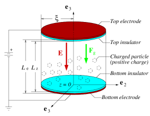
Figure 13: (Color online) Configuration used to plot $P_{s}\left(z_{i}\right)$ defined in Eq. (42).

Having defined $Q,$ $m,$ and $\mathbf{E},$ the configuration illustrated in Fig. 13 is referred to plot $P_{s}\left(z_{i}\right),$ Eq. (42). The parameters for the configuration are given the following values:

$$\left\{\begin{array}[]{c}L_{\textup{e}}=100\,\mu\textup{m},\;L_{\textup{z}}=90\,\mu\textup{m},\;\xi=50\,\mu\textup{m},\\ \rho_{\textup{m}}=2.7\,\textup{g}\,\textup{cm}^{-3},\;r=50\,\textup{nm},\\ T=42\,^{o}\textup{C},\;N=1000,\;n_{\textup{e}}=15.\end{array}\right.$$

For the purpose of plotting $P_{s}\left(z_{i}\right)$ defined in Eq. (42), I shall assume, see Eq. (41),

$$Q_{\textup{eff}}=0.97Q,$$

where $Q$ is defined in Eq. (43). The voltages of $V_{0}=0\,\textup{V},$ $0.1\,\textup{V},$ $0.2\,\textup{V},$ $0.3\,\textup{V},$ and $0.5\,\textup{V}$ are considered for the top electrode (the bottom electrode is grounded). With $V_{0}$ thus defined, the electric field generated inside chamber is given by Eq. (45). The gravity of $g=9.8\,\textup{m}/\textup{s}^{2}\geq 0$ was assumed inside the chamber. The directions for the electric field $\mathbf{E}$ and the gravitational force $\mathbf{F}_{\textup{g}}$ are determined from Eqs. (21) and (22). Since both $E$ and $g$ are positive, according to the convention defined in Eqs. (21) and (22), the electric field $\mathbf{E}$ and the gravitational force $\mathbf{F}_{\textup{g}}$ are both directed in $-\mathbf{e}_{3},$ which is the negative $z$ axis. The $P_{s}\left(z_{i}\right)$ of Eq. (42) is computed numerically utilizing Simpson method for the integral.thomas-finney The Simpson method routine was coded in FORTRAN 90. That being said, the results are summarized in Figs. 14 and 15, where the three smaller peaks of Fig. 14 are magnified and replotted in Fig. 15.

At $V_{0}=0\,\textup{V},$ that is, when there is no electric field inside the chamber other than the static fields from particles, the particles are distributed to occupy the entire volume of the chamber. This is indicated by the peak occurring at the physical height of the chamber, $h_{\textup{c}}=z=L_{\textup{z}}=90\,\mu\textup{m}.$

At $V_{0}=0.2\,\textup{V},$ an electric field of roughly $E\approx 2000\,\textup{V}\,\textup{m}^{-1}$ is generated inside the chamber. Because particles are positively charged, they are compressed in the direction of electric field, i.e., the $-z$ direction. This force, which induced particle volume compression, eventually gets counter balanced by the Coulomb repulsion and the compression ceases. For the case where control electrode is held at $V_{0}=0.2\,\textup{V},$ the compression ceases at roughly $h_{\textup{c}}=z\approx 63\,\mu\textup{m}$ (see Fig. 15) and this marks the most probable height of the compressed volume for the case. Finally, with $V_{0}=0.5\,\textup{V}$ applied to the control electrode, the compressed volume state is reached where all particles are cluttered near the floor of the chamber, thereby resulting in very high particle density, as illustrated in Fig. 14.

If charged particles are to be useful for any display applications, the charged particle system must be insensitive to gravitational effects, if not negligible. The effect of gravity on the most probable height for the compressed volume has been investigated by reversing the direction of gravity (but, keeping all other conditions unchanged) in Fig. 15. The case where $V_{0}=0.2\,\textup{V}$ was selected for comparison. The result is shown in Fig. 16, where it shows that the most probable height for the compressed volume is only negligibly affected by the gravity.

The influence of cylinder radius $\xi$ on the most probable height for the compressed volume has also been investigated. Again, the case of $V_{0}=0.2\,\textup{V}$ was selected from Fig. 15 for comparison by considering $\xi=50,$ $60,$ and $70\,\mu\textup{m}.$ All other conditions were kept unmodified. The result, Fig. 17, reveals a decrease in height for the most probable compressed volume with increasing $\xi$ as expected.

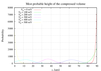
Figure 14: (Color online) Most probable height of the compressed volume containing charged particles.

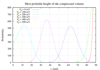
Figure 15: (Color online) The three small peaks in Fig. 14 are magnified for detail. Each peak represents the most probable height for the compressed volume, where there are $N$ charged nanoparticles inside the volume.

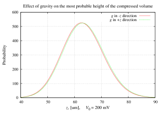
Figure 16: (Color online) Gravity has negligible effect on most probable height of the compressed volume.

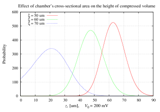
Figure 17: (Color online) The height of the compressed volume decreases with the increased radius of the cylindrical chamber.

II.4 Transmission intensity

The intensity of light transmitted through a medium filled with charged particles goes like, Eq. (2),

$$I=I_{0}\exp\left(-\frac{C}{h_{\textup{c}}}\right), C=\frac{36n\pi khNv_{\textup{p}}}{\lambda\left(n^{2}+2\right)^{2}A},$$ (46)

where both $C$ and $h_{\textup{c}}$ have unit of meter, and $h_{\textup{c}}$ is the height of the compressed volume containing charged particles. Referring to Fig. 15, the compressed height $h_{\textup{c}}$ corresponds to the $z$ axis where the probability curve is maximum. In principle, the compression height $h_{\textup{c}}$ can be varied continuously by controlling the voltages applied to the control electrode. This implies the intensity of light output from the proposed optical shutter can be varied continuously, thereby generating continuous grayscale levels for the device. In reality, the number of grayscale levels that can be achieved in the presented optical shutter is given by Eq. (15),

$$N_{\textup{gray}} =\frac{h-\delta}{\triangle h_{\textup{c}}},$$

where the fineness of $\triangle h_{\textup{c}}$ is limited by the system design.

This work is not the first kind to address potential applications with charged particles. SzirmaiSzirmai experimented with alumina powders to study electrosuspension as early as 1990’s. In Szirmai’sSzirmai experiment, alumina powder of $3\,\mu\textup{m}$ in diameter was placed inside an electrically insulating cylindrical vessel, which is similar in configuration with Fig. 13. The initial charging of alumina powder was done by a process of field emission, which can be achieved by applying high voltage to the control electrodes(field emission is the phenomenon in which electrons get emitted from the surface of host material, such as nanoparticles, due to the presence of high electric fields). Szirmai,Szirmai however, does not quantitatively address the compression states of volume containing charged particles in terms of the design parameters, as his motive was not in discussing possible applications of charged particles for displays. In his experiment, the control electrodes, in principle, could be supplied with whatever high voltages required by it to do the job; therefore, the quantitative understanding of how design parameters, such as $L_{\textup{e}},$ $L_{\textup{z}},$ $\xi,$ $\rho_{\textup{m}},$ $r,$ $T,$ $N,$ $n_{\textup{e}},$ $V_{0},$ and $Q_{\textup{eff}}\propto Q,$ enter into the picture of particle volume compression never was an issue.

The competition has always been fierce and it will always remain so among different display manufacturers. In the near future, when paperlike displays become dominant, the most important deciding factor to who stays in and goes out of business would be determined by the power efficiency of their products. That being said, a low operation voltage for the control electrodes is crucial for all E-paper technologies and the proposed device based on charged particles is no exception. The light intensity out of each sub-pixel based on proposed charged particle display technology varies as illustrated in Eq. (46), where $h_{\textup{c}}$ is the most probable compression height corresponding to the voltage difference of $V_{0}$ applied to the control electrodes, see Fig. 14. With the $V_{0}$ restricted to certain range, say $0\,\textup{V}\leq V_{0}\leq 1\,\textup{V},$ one cannot arbitrarily choose the other parameters which constitute the design parameters, i.e., $L_{\textup{e}},$ $L_{\textup{z}},$ $\xi,$ $\rho_{\textup{m}},$ $r,$ $T,$ $N,$ $n_{\textup{e}},$ and $Q.$ For example, if too many electrons are removed from each of the aluminum particles, i.e., $n_{\textup{e}},$ the voltage of $V_{0}=1\,\textup{V}$ applied to one of the control electrodes (the other grounded) may not be sufficient enough to overcome the Coulomb repulsion between particles and compress the particle volume to a level where dark state is reached, assuming $V_{0}=0\,\textup{V}$ defines the brightest state. On the other end, if too many charged particles are present in a chamber, i.e., the particle number $N,$ the brightest state achieved by setting $V_{0}=0\,\textup{V}$ for the control electrode may be too dark. The quantitative description of the height $h_{\textup{c}}$ of the compressed particle volume in terms of the so called “design parameters” thru the expression $P_{s}\left(z_{i}\right),$ Eq. (42), ables the design of particle based display with potential to generate continuous grayscale.

II.5 Bistability

The presented optical shutter based on charged particles portrays bistability at all states, including the gray states. This is possible because the two optically transparent electrodes act as a capacitor, which has the property of sustaining electric fields even when the device is removed of the power supply. To illustrated how the bistability is achieved for all states, including the gray states, the illustration shown in Fig. 18 is considered. I shall begin with an isolated capacitor, in which the two electrodes of the capacitor are electrically neutral, resulting in zero electric field inside the region between the two electrodes. With the switch closed, the top electrode is quickly accumulated with a net positive charge, $+Q,$ and the bottom electrode gets accumulated with a net negative charge, $-Q.$ The potential difference between the two electrodes results in the creation of electric field inside the capacitor, as illustrated in stage 2 of Fig. 18. Assuming the charged particles reside in the region between the two electrodes, the electric field generated inside the capacitor is responsible for the compression of volume containing charged particles. Now, when the switch is opened, the net charge of $+Q$ remains in the top electrode and the net charge of $-Q$ remains in the bottom electrode, provided the capacitor is ideal, i.e., free from the leakage of electrical current. Therefore, for an ideal capacitor, the electric field is maintained forever inside the region between the two electrodes, thereby sustaining the gray states even when the device is removed of the power supply.

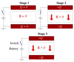
Figure 18: (Color online) The bistability is maintained by the electric field stored in the capacitor.

In the real system, the role of switch is played by a semiconductor transistor, which is very far from being an ideal switch and it has finite leakage of current. This deficiency in semiconductor transistor makes the proposed device only semi-bistable, meaning the device must be refreshed regularly. This, however, is about to change with the current developments in micro electromechanical systems (MEMS) based switches, which literally has zero leakage current for the open state.MEMS-switch Initially, the MEMS based switch has been developed in an attempt to replace the dynamic random access memory (DRAM) architecture for the memory sector of business. However, as it lacks in switching speed, it will be a while before MEMS based switches can permanently replace the DRAMs. As for its use as a switch in display technology, the MEMS based switches already show plenty of speed. Combined with MEMS based switches, which has zero leakage current for the open switch mode, the proposed optical shutter based on charged particles opens up the possibility of realizing the bistability mode for all states, including the grayscale states.

III Concluding Remarks

The pioneering work by Szirmai,Szirmai Hattori et al.,QR-LPD2 ; QR-LPD3 ; QR_LPD4 and others have exposed the potential applications with charged particles. Utilizing charged particles in display technologies, however, requires a quantitative understanding of how design parameters, such as $L_{\textup{e}},$ $L_{\textup{z}},$ $\xi,$ $\rho_{\textup{m}},$ $r,$ $T,$ $N,$ $n_{\textup{e}},$ $V_{0},$ and $Q_{\textup{eff}}\propto Q,$ enter into particle volume compression. In this work, an expression for the compressed state, which incorporates the design parameters, has been presented. The result should find its role in the development of displays based on charged particles.

IV Acknowledgments

The author acknowledges the support for this work provided by Samsung Electronics, Ltd.

References

- (1) I. Ota, U.S. Patent No. 3668106 (June/1976); U.S. Cl. 204/299.
- (2) N. Sheridon, U.S. Patent No. 4126854 (1978.11.21).
- (3) J. Jacobson and H. Yoshizawa, U.S. Patent No. 6241921 (2001.06.05).
- (4) J. Ding, C. Liao, S. Jeng, Y. Chen, and C. Lu, U.S. Patent No. 20060087490 (2006.04.27).
- (5) H. Mizuno, U.S. Patent No. 7023609 (2006.04.04).
- (6) H. Matsuda, U.S. Patent No. 20070109622 (2007.05.17).
- (7) B. Comiskey, J. Albert, H. Yoshizawa, and J. Jacobson, Nature (London) 394, 253 (1998).
- (8) T. Whiteside, M. Walls, R. Paolini, S. Sohn, H. Gates, M. McCreary, and J. Jacobson, SID Int. Symp. Digest, 35, 133 (2004).
- (9) T. Kosc, Opt. and Photonics News, 16, 18 (2005).
- (10) R. Sakurai, H. Hiraoka, T. Kobayashi, H. Yamazaki, and H. Kitano, U.S. Patent No. 20080174854 (2008.07.24).
- (11) R. Hattori, S. Yamada, Y. Masuda, and N. Nihei, J. Soc. Inf. Disp. 12, 75 (2004).
- (12) R. Hattori, S. Yamada, Y. Masuda, N. Nihei, and R. Sakurai, J. Soc. Inf. Disp. 12, 405 (2004).
- (13) R. Hattori, S. Yamada, Y. Masuda, N. Nihei, and R. Sakurai, SID Int. Symp. Digest 35, 136 (2004).
- (14) S. Kwon, S. Lee, W. Cho, B. Ryu, and M. Song, SID Int. Symp. Digest 37, 1838 (2006).
- (15) S. Johnson, Stephen John on Digital Photography (O’Reilly Media, ISBN-13: 978-0596523701, 2006).
- (16) S. Kaneko, M. Asakawa, R. Hattori, Y. Masuda, N. Nihei, A. Yokoo, S. Yamada, Proceeding of IDW08, pp.1267-1270 (Dec. 2008).
- (17) M. Nishii, R. Sakurai, K. Tanaka, S. Ohno, S. Tsuchida, Y. Masuda, I. Tanuma, and R, Hattori, Proceedings of the SID ’08 Digest, 1819 (2008): (ISSN/008-0966X/08/3903-1819).
- (18) R. Hattori, S. Yamada, Y. Masuda, and N. Nihei, Proceedings of the SID ’03 Digest, 846 (2004): (ISSN/0003-0966X/03/3402-0846).
- (19) W. Chim, “A Flexible Electronic Paper with Integrated Display Driver using Single Grain TFT Technology,” MSc. Thesis, Computer Engineering, Dept. of Electrical Engineering, Delft University of Technology (2009).
- (20) S. Cho, South Korean Patent No. 1020080105475 (2008.10.27).
- (21) C. Bohren and D. Huffman, Absorption and Scattering of Light by Small Particles (John Wiley & Sons, New York, USA, 1998).
- (22) P. Stoller, V. Jacobsen, and V. Sandoghdar, Opt. Lett. 31, 2474 (2006).
- (23) P. Johnson and R. Christy, Phys. Rev. B 6, 4370 (1972).
- (24) R. DeRosa, P. Schader, and J. Shelby, J. Non-Cryst. Solids 331, 32 (2003).
- (25) Y. Shin, D. Lee, K. Lee, K. Ahn, and B. Kim, J. Ind. Eng. Chem. (Seoul, Repub. Korea) 14, 515 (2008).
- (26) B. Alince and R. Tino, Colloids Surf., A 218, 1 (2003).
- (27) H. Miyake, Y. Tanaka, T. Takada, and R. Liu, Proceedings of 2005 International Symposium on Electrical Insulating Materials (Kitakyushu, Japan) 1, 49 (2005).
- (28) H. Miyake, Y. Tanaka, and T. Takada, IEEE Trans. Dielectr. Electr. Insul. 14, 520 (2007).
- (29) F. Reif, Fundamentals of statistical and thermal physics (McGraw-Hill, New York, 1965).
- (30) G. Thomas and R. Finney, Calculus and analytic geometry, 7th Ed, (Addison-Wesley, USA, 1988).
- (31) S. Szirmai, Industry Applications Conference, 2000. Conference Record of the 2000 IEEE (Rome, Italy) 2, 851 (2000).
- (32) I. Cho, T. Song, S. Baek, and E. Yoon, Proceedings of the 18th IEEE International Conference on Micro Electro Mechanical Systems, 32 (2005): (DOI 10.1109/MEMSYS.2005.1453860).