The Northern Sky Optical Cluster Survey III:
A Cluster Catalog Covering Pi Steradians

Abstract

We present the complete galaxy cluster catalog from the Northern Sky Optical Cluster Survey, a new, objectively defined catalog of candidate galaxy clusters at $z\hbox{ \hbox to0.0pt{\raise 1.82986pt\hbox{$<$}\hss}\lower 2.79857pt\hbox{$\sim$} }0.25$ drawn from the Digitized Second Palomar Observatory Sky Survey (DPOSS). The data presented here cover the Southern Galactic Cap, as well as the less-well calibrated regions of the Northern Galactic Cap. In addition, due to improvements in our cluster finder and measurement methods, we provide an updated catalog for the well-calibrated Northern Galactic Cap region previously published in Paper II. The complete survey covers 11,411 square degrees, with over 15,000 candidate clusters. We discuss improved photometric redshifts, richnesses and optical luminosities which are provided for each cluster. A variety of substructure measures are computed for a subset of over 11,000 clusters. We also discuss the derivation of dynamical radii $r_{200}$ and its relation to cluster richness. A number of consistency checks between the three areas of the survey are also presented, demonstrating the homogeneity of the catalog over disjoint sky areas. We perform extensive comparisons to existing optically and X-ray selected cluster catalogs, and derive new X-ray luminosities and temperatures for a subset of our clusters. We find that the optical and X-ray luminosities are well correlated, even using relatively shallow ROSAT All Sky Survey and DPOSS data. This survey provides a good comparison sample to the MaxBCG catalog based on Sloan Digital Sky Survey Data, and complements that survey at low redshifts $0.07<z<0.1$.

1. Introduction

The construction of large catalogs of galaxy clusters for use in studies of cosmology, large scale structure, and galaxy evolution has often proven to be a difficult task (see Gal, 2008, for a review). Indeed, the last such catalog generated using optical data, and covering the entire high-galactic-latitude Northern sky was that of Abell (1958), updated in 1989 (Abell, Corwin & Olowin, 1989). More recently, the Northern ROSAT All-Sky (NORAS) Galaxy Cluster Survey (Böhringer et al., 2000) has provided an X-ray selected catalog covering a similar region, but with many fewer clusters, while the largest catalog using purely digital observations (Koester et al., 2007b) covers a smaller area, albeit with much better photometry.

Because much improved optical data has become available, with automated techniques to generate objective, well-characterized cluster samples, we undertook the generation of a modern, optically selected cluster catalog, the Northern Sky Optical Cluster Survey (NoSOCS Gal et al., 2000, 2003, hereafter Papers I and II), and its deeper extension (Lopes et al., 2004, hereafter Paper IV). The need for a modern cluster survey covering a significant portion of the sky is striking. The catalog from Paper II has already been used to suggest a connection between short-duration gamma-ray bursts and clusters (Gehrels et al., 2005; Bloom et al., 2006), to search for giant arcs (Hennawi et al., 2008), to associate compact groups and large-scale structure (de Carvalho et al., 2005; Andernach & Coziol, 2006), and to examine X-ray and optical cluster properties (Lopes et al., 2006). Here we present the second and final installment of this catalog, including photometric redshifts, richnesses, optical luminosities and substructure measures. Although superior imaging data is now available from the Sloan Digital Sky Survey (SDSS, York et al. 2000), the imaged area covers less than half of the Northern sky, and is not expected to ever reach the area coverage of our catalog. The currently published cluster catalog from SDSS (Koester et al., 2007b) covers $\sim 7500$ deg², containing nearly 14,000 clusters. That survey, using the MaxBCG technique, has a lower redshift cutoff of $z=0.1$; our survey extends down to $z=0.07$. This provides a sample of more local clusters whose properties can be examined in detail (Lopes et al., 2008), especially using the extensive SDSS spectroscopic database.

The regions covered in this paper are shown in Figure 1. Three separate areas are covered: (1) The well-calibrated North Galactic Pole (NGP) region already described in Paper II (dotted lines); (2), the portion of the NGP with less well calibrated plates, not covered in Paper II (solid lines); and (3), the Southern Galactic Pole region (SGP, dashed lines). The area covered by the NGP-poor region is 2813$\Box^{\circ}$, while the SGP covers 2917$\Box^{\circ}$. Together with the 5681$\Box^{\circ}$ surveyed in Paper II, the final NoSOCS catalog covers 11411 square degrees. The distribution of clusters in the survey is shown in Figures 2 and 3, in equatorial and galactic coordinates, respectively. Only clusters with richness $N_{gals}>20$ are shown for clarity.

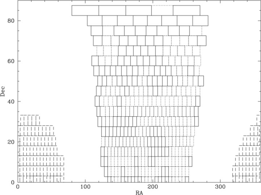
Figure 1.— The distribution of DPOSS plates used in NoSOCS, showing the NGP well-calibrated (solid lines), poorly calibrated (dotted lines) and SGP (dashed lines) regions.

Figure 2.— Aitoff projection of the complete NoSOCS cluster catalog in equatorial coordinates.

Figure 3.— Aitoff projection of the complete NoSOCS cluster catalog in galactic coordinates.

The survey methodology is described in §2. Although the overall detection technique is very similar to that discussed in Paper II, we have modified our definition of bad areas due to very bright objects, reducing contamination by spurious detections. Changes to the photometric redshift estimation yield more robust (and realistic) errors. The richness estimator has also been improved, providing robust error estimates, as well as total $r$-band optical luminosities. Then, in §3, we discuss two new sets of parameters computed for our cluster sample: estimates of cluster substructure and the dynamical radius $r_{200}$.

In §4 we describe the general characteristics of our cluster sample, and present consistency tests for the three sky regions utilized. The selection functions describing the completeness as a function of richness and redshift are presented, as is an estimate of the contamination by projection effects. Our complete and final cluster catalog, including an updated version covering the area from Paper II, is presented. This cluster sample is compared to other optically-selected catalogs in §5. In particular, we compare our catalog to the SDSS MaxBCG catalog of Koester et al. (2007b), the only modern optical cluster catalog covering a similar area and redshift range. We then examine the correlation between our redshifts and richnesses and the X-ray measurements from the Northern ROSAT All-Sky Galaxy Cluster Survey (NORAS, Böhringer et al. 2000). Because NORAS consists of many fewer clusters than our catalog, we use our optical positions to measure X-ray fluxes and upper limits from RASS for a significant subsample of NoSOCS.

2. Survey Methodology

The detection of galaxy clusters in modern optical imaging surveys typically utilizes the existence of a tight color–magnitude relation for cluster galaxies, noted nearly half a century ago (Baum, 1959; Bower et al., 1992). Surveys at low and high redshift have made use of this observation to efficiently detect clusters, while achieving low contamination (false positive) rates (Gladders & Yee, 2000; Hansen et al., 2005). We use the galaxy catalogs from the Digitized Second Palomar Observatory Sky Survey (DPOSS, Djorgovski et al., 1999) as the basis for our survey. Unfortunately, the limited photometric accuracy ($\sigma_{mag}\sim 0.25^{m}$ at $r=19.5$, Gal et al. 2004) of DPOSS forces us to rely solely on the two-dimensional projected galaxy distribution for cluster detection. Details of the photometric calibration and star/galaxy separation are discussed in Gal et al. (2004) and Odewahn et al. (2004) respectively. In brief, the positions of the galaxies are used to generate adaptive kernel (AK) density maps (Silverman, 1986) which outputs images in units of projected galaxy density. We then run SExtractor (Bertin & Arnouts, 1996) on these images, detecting peaks which are identified as potential galaxy clusters. We refer the reader to Papers I and II for more comprehensive descriptions of the cluster detection. Photometric redshifts are estimated using the background-corrected mean $r$ magnitude and median $g-r$ color of the galaxies within a 0.5$h^{-1}$Mpc radius of the cluster center; details on improvements to this estimator from our previous work are described below. The photometric redshifts are used to recenter the clusters, also discussed later. Richnesses are computed by counting galaxies with $M^{*}-1\leq M^{*}_{r}\leq M^{*}+2$ within the same radius, with corrections applied for higher (and now lower) redshift clusters where the faint (or bright) end of this magnitude range is beyond our catalog limits. We note that galaxy colors are used only in the post-detection steps to estimate photometric redshifts for the clusters.

2.1. Enhanced Removal of Bad Areas

In the process of generating the catalog presented in Paper II, it became obvious that the DPOSS catalogs were insufficient for finding very bright stars and galaxies, which are typically deblended into numerous fainter components. In later work, Paper IV utilized the Tycho-2 catalog to excise candidate higher-redshift clusters in the area of bright stars after detection. To avoid spurious cluster detections due to these artifacts, we now rely on the Tycho-2 and RC3 catalogs to exclude regions in the vicinity of bright objects before performing cluster detection. Specifically, around bright stars we exclude circular regions whose area depends on the star’s Tycho magnitude; $2^{\prime}$ radius for $m_{Tycho}<7.0$, $1.5^{\prime}$ for $7.0\leq m_{Tycho}<8.0$, and $1.0^{\prime}$ for $8.0\leq m_{Tycho}<9.5$. These radii were chosen by visually inspecting plate images and the resulting galaxy catalogs to determine the sizes of regions contaminated by the bright stars. In addition, larger regions around bright galaxies in the RC3 catalog (de Vaucouleurs et al., 1991) were excised, corresponding to $5\times r_{\rm{RC3}}$ for $r_{\rm{RC3}}<25^{\prime\prime}$ and $8\times r_{\rm{RC3}}$ for $r_{\rm{RC3}}\geq 25^{\prime\prime}$.

The removal of objects in these contaminated regions results in empty holes in the galaxy catalogs. An undesired consequence is that in these areas the adaptive kernel artificially increases the smoothing radius (which is inversely proportional to the local density). To remedy this problem, we generate simulated galaxy catalogs using the Raleigh-Levi distribution (Postman, Lauer, Oegerle, & Donahue, 2002, Paper II), and use these to fill the excised areas as well as the densitometry spot region on each plate. With this technique, the regions which would otherwise be empty instead contain galaxies with the average projected density for each plate.

After cluster detection is completed, the final catalog is again checked against the list of bad areas. For some very extended, nearby galaxies, or very bright stars, we found through visual inspection that the exclusion area described above was not always sufficient. We therefore increased the radius of these areas, by a factor of 1.5 for the Tycho-2 stars, and to $10\times r_{\rm{RC3}}$ for the RC3 galaxies. In addition, we created additional bad areas from catalogs of Galactic globular and open clusters, as these objects were found to be contaminants in our previous catalogs. Any candidates found within an exclusion radius defined by the sizes of these Galactic clusters was also eliminated. Visual inspection of candidates flagged in this last step shows that the vast majority were indeed bad. A total of 404 candidates, 2.5% of the sample, are removed from the catalog in this step.

2.2. Photometric Redshift Improvements

A number of small but significant changes were made to the algorithm presented in Paper II. These modifications enhance the photometric redshift measurements based on DPOSS photometry and provide more robust error estimates. First, we re-derived the empirical relation between the median $g-r$ color, mean $r$ magnitude of the cluster galaxies, and the spectroscopic redshift (equation 1 in Paper II). This was prompted in part by modifications to the background estimator (described below), which results in changes to the global properties of the cluster galaxy populations. Our larger sky coverage also allowed us to restrict the spectroscopic cluster sample to those clusters with more than three concordant redshifts in the compilation of Struble & Rood (1991), resulting in a training sample of 254 clusters. We also found that the redshift estimator was more reliable when restricted to galaxies with $m_{r}\leq 19.5$, as opposed to $m_{r}\leq 20.0$ used before. The recalibrated photometric redshift relation used here is

$${z_{phot}=0.3273\times(g-r)_{med}-0.0702\times r_{mean}-1.2685}$$ (1)

with a $Q_{\sigma}(z_{spect}-z_{phot})/(1+z_{spec})=0.023$, an improvement of $\sim 30\%$ over the results in Paper II.

As noted above, one major modification to our technique involves measurement of the fore- and background galaxy contamination in the cluster area. In Papers I and II, we used color and magnitude distributions from each DPOSS plate ($\sim 30$ deg²), scaled to the area of each cluster on that plate, as the background correction. This ignores the contribution of local large scale structure to the background of each cluster, which can introduce systematic errors since galaxy colors and luminosities are strongly correlated with local density (Dressler, 1980; Blanton et al., 2005). We therefore implemented a local background estimator, as follows:

1. A random position is chosen within a background annulus of width $1.3^{\circ}$ starting 3$h^{-1}$ Mpc from the cluster center.

2. A box of size $20^{\prime}\times 20^{\prime}$ is placed at the random location

3. A check is performed to see if the box intersects a bad area (hole) in the survey; if so, we return to step 1.

4. The distribution of colors and magnitudes is generated for the galaxies in this box.

5. The procedure is iterated until ten background regions are successfully measured.

6. The $3\sigma$-clipped medians of the distributions from the ten background regions are used as the background correction for that cluster.

The redshift estimator is run ten times for each cluster candidate. Changes in the placement of the randomly located background measurement regions result in variations of the background galaxy color and magnitude distributions, which effect the final photometric redshift. By repeating the measurement, we derive an estimate of the random error in $z_{phot}$ due to the background correction, which we then add in quadrature to the scatter from the redshift – photometric properties relation. Although some of the latter is likely due to difficulties with properly estimating the background contribution, we prefer to estimate the redshift errors conservatively, adding the errors as if they were independent. We note that such problems are likely to be significantly reduced in modern digital imaging surveys,where the photometric errors are an order of magnitude smaller than for DPOSS (Gal et al., 2003; Adelman-McCarthy et al., 2007). As a final change to the redshift estimator, we allow more iterations for convergence (15 instead of 10). This was found to increase the number of successful redshift estimates, while allowing further iteration simply grew the computational requirements with little improvement.

For some clusters, the photometric redshift estimator does not converge in all ten of the runs. The final photometric redshift is taken as the mean $z_{phot}$ from the $n_{successful}$ runs. The redshifts and their associated errors are provided in Columns 5 and 6 of Table 3. For those clusters where the $z_{phot}$ estimate always failed, these three columns are all set to 0. Such clusters are likely to be spurious detections or have contaminated photometry from bright stars, telescope reflections or other artifacts.

2.3. Cluster Centroids

During the photometric redshift measurement process, the cluster positions are also recomputed. At each iteration of the $z_{phot}$ computation, we calculate the median position of the galaxies within a 1$h^{-1}$ Mpc radius of the previously determined center, and this is taken as the new cluster centroid for the next iteration of the photometric redshift estimation. To avoid large offsets, the maximum change in position is limited to 2 arcminutes; if the recomputed center is further from the previous location, then the center is not moved. The above steps are repeated for each of the $n_{successful}$ photometric redshifts, and the final cluster position is recorded as the mean of the corresponding $n_{successful}$ positions. In those cases where the photometric redshift estimator does not converge, we retain the original position (from running SExtractor on the density map).

2.4. Richness and Luminosity Measures

Richnesses and luminosities are computed using the basic methods described in Lopes et al. (2006), with some further refinements, and adjusted for the lower redshift range probed here. The procedure consists of five steps for each cluster, described below.

1. We use $z_{phot}$ to determine the apparent magnitude $m^{*}_{r}$, the aperture corresponding to 0.50 $h^{-1}$ Mpc, and the $k$-corrections $k_{e}$ and $k_{s}$ for elliptical and late-type galaxies (Sbc) at the cluster redshift. We select all galaxies within 0.50 $h^{-1}$ Mpc of the cluster center and with $m^{*}_{r}-1+k_{s}\leq m_{r}\leq m^{*}_{r}+2+k_{e}$. The $k$-corrections are applied to individual galaxies at a later stage, so these limits guarantee that we select all galaxies that can fall within $m^{*}_{r}-1\leq m_{r}\leq m^{*}_{r}+2$. The number of galaxies selected in the cluster region is N_clu.

2. We estimate the background contribution locally. We randomly select ten $20^{\prime}\times 20^{\prime}$ boxes (avoiding bad areas) in a 1.3^∘-wide annulus, starting 3 h^-1 Mpc from the cluster center. Galaxies are selected within the same magnitude range as used for computing N_clu. The median counts from the ten boxes are scaled to the cluster area to generate the background estimate (N_bkg). We adopt the interquartile range (IQR, which is the range between the first and third quartiles) as a measure of the error in N_bkg, which we term $Q_{\sigma,bkg}$. The background corrected cluster counts (N_clu - N_bkg) is called N_corr.

3. Next, a bootstrap procedure is used to statistically apply k$-$corrections to the galaxy populations in each cluster. In each of 100 iterations, we randomly select N_corr galaxies from those falling in the cluster region (N_clu). An elliptical k$-$correction is applied to 80$\%$ of the N_corr galaxies, while an Sbc k$-$correction is applied to the remaining 20$\%$. Finally, we use these k$-$corrected magnitudes to count the number of galaxies with $m^{*}_{r}-1\leq m_{r}\leq m^{*}_{r}+2$. The final richness estimate N_gals is given by the median counts from the 100 iterations. The richness error from the bootstrap procedure alone is given by $Q_{\sigma,boot}$. The richness error is the combination of this error and the background contribution, so that $Q_{\sigma}$ = $\sqrt{Q_{\sigma,boot}^{2}+Q_{\sigma,bkg}^{2}}$. At this point, the richness error includes contributions from the $k$-correction and the background galaxy correction, but not the redshift uncertainty, which is incorporated in Step 5.

4. If the cluster is too nearby or too distant, either the bright ($m^{*}_{r}-1+ks$) or faint ($m^{*}_{r}+2+ke$) magnitude limit, respectively, will exceed one of the survey limits ($15.0\leq m_{r}\leq 19.5$). We then apply the appropriate incompleteness correction to the richness estimate:

   $$\gamma_{1}={\int_{m_{r}^{*}-1}^{m_{r}^{*}+2}\Phi(m)dm\over\int_{15}^{m_{r}^{*}+2}\Phi(m)dm}$$ (2)

   $$\gamma_{2}={\int_{m_{r}^{*}-1}^{m_{r}^{*}+2}\Phi(m)dm\over\int_{m_{r}^{*}-1}^{20}\Phi(m)dm}$$ (3)

   We call $\gamma_{1}$ and $\gamma_{2}$ the low and high magnitude limit correction factors.

5. The above steps are repeated using each of the $n_{successful}$ photometric redshifts. The final cluster richness is recorded as the mean of the corresponding $n_{successful}$ richnesses. We compute the mean of the richness errors from Step 3, as well as the dispersion among the richnesses from the $n_{successful}$ iterations. The former quantifies how much richness variation we expect based solely on cosmic variance, assuming there is no error in the redshift estimates, while the latter reflects the richness error due to scatter in the photometric redshifts. Because these are two independent sources of error, we add them in quadrature to derive the final richness error $Q_{\sigma,Ngals}$.

Total $r$-band luminosities (in solar units) and their errors are computed similarly to the richnesses. No attempt is made to fit and integrate luminosity functions for the individual clusters.

2.5. Completeness and Contamination

The global contamination rate is estimated following Lopes et al. (2004). For each plate, we use the Raleigh-Levy (RL) distribution to generate $N_{real,i}$ x,y coordinates, where $N_{real,i}$ is the number of galaxies in the DPOSS catalog for plate $i$. Each galaxy in the RL catalog is assigned a magnitude selected randomly from the real data. The density mapping and cluster detection is performed on the RL catalog for each plate, and the detected ’clusters’ are assigned photometric redshifts at random from the real clusters in that plate. To estimate the global contamination rate for our sample, we ran this procedure on a plate-by-plate basis for the entire NoSOCS area. The results are shown in Figure 4, where the top panel shows the distribution of real clusters (solid line) and false clusters (from the RL simulations, dotted line), as a function of richness. The total contamination rate is 8.4%, consistent with our goal of achieving $\leq 10\%$ contamination when setting the cluster detection parameters. The bottom panel shows the contamination rate as a function of richness. For very rich clusters ($N_{gals}>50$) the contamination rate is negligible, and only rises above 5% for $N_{gals}<20$.

The redshift- and richness-dependent completeness functions for each plate are provided in Table 1. The first column gives the plate number; for each plate, there are 42 entries, using six richnesses ($N_{gals}=15,25,35,50,80,120$) given in the second column, at seven redshifts ($z=0.08$ to 0.32 with $\delta z=0.04$) given in the third column. The fourth column gives the recovery rate (in percent) of clusters with the given richness, at the listed redshift, for that specific plate. To use a large cluster sample for cosmology requires knowledge of the mass-dependent selection function (SF). Currently, there are two methods to generate these, either by empirically calibrating a mass-observable relation, or using large simulations to construct mock galaxy catalogs from which clusters are selected. Koester et al. (2007a) use the latter to estimate the purity and completeness of the SDSS MaxBCG cluster catalog, but we do not have such simulations corresponding to our data. Using X-ray observations, we are in the process of developing an optimized richness estimator to generate an $N_{gals}-$ Mass relation. However, that work is beyond the scope of this paper.

Table 1Completeness Functions

Plate	Richness	Redshift	Completeness
005	015	0.08	34.0
005	015	0.12	10.0
005	015	0.16	10.0
005	015	0.20	2.0
005	015	0.24	0.0
005	015	0.28	0.0
005	015	0.32	0.0
005	025	0.08	78.0
005	025	0.12	68.0
005	025	0.16	50.0
005	025	0.20	12.0
005	025	0.24	8.0
005	025	0.28	0.0
005	025	0.32	0.0
005	035	0.08	96.0
005	035	0.12	82.0
005	035	0.16	72.0
005	035	0.20	30.0
005	035	0.24	8.0
005	035	0.28	8.0
005	035	0.32	0.0
005	055	0.08	98.0
005	055	0.12	92.0
005	055	0.16	92.0
005	055	0.20	82.0
005	055	0.24	46.0
005	055	0.28	10.0
005	055	0.32	6.0
005	080	0.08	100.0
005	080	0.12	98.0
005	080	0.16	94.0
005	080	0.20	92.0
005	080	0.24	64.0
005	080	0.28	34.0
005	080	0.32	8.0
005	120	0.08	100.0
005	120	0.12	100.0
005	120	0.16	98.0
005	120	0.20	100.0
005	120	0.24	90.0
005	120	0.28	64.0
005	120	0.32	24.0

Figure 4.— Contamination of the entire NoSOCS catalog by false clusters. The top panel shows the distribution of real clusters (solid line) and false clusters (from the RL simulations, dotted line), as a function of richness. The total contamination rate is 8.4%, consistent with our goal of achieving $\leq 10\%$ contamination when setting the cluster detection parameters. The bottom panel shows the contamination rate as a function of richness. For very rich clusters ($N_{gals}>50$) the contamination rate is negligible, and only rises above 5% for $N_{gals}<20$.

2.6. Other Changes

Following Paper II, we generate ten additional AK maps for each plate, using a set of galaxy catalogs for each plate with random photometric zero-point offsets added to the $r$-band magnitudes, drawn from the known photometric error distribution for DPOSS given in Gal et al. (2004). In Paper II we required that a cluster candidate be detected in seven of the ten zero-point-error-added maps in addition to the original map. In the final catalog, we now require only that a candidate be detected in any seven of the eleven maps, as there is no a priori reason to give preference to the original map. This typically results in $\sim 5-10\%$ additional candidates per plate.

Table 2Statistics From Three NoSOCS Regions

Region	Nclusters	Area ($deg^{2}$)	$\rho$ (N deg-2)	$z_{med}$	$z_{Q\sigma}$	$N_{gals,med}$	$N_{gals,Q\sigma}$	P($z_{phot}$)	P($N_{gals}$)
NGP, good	7985	5681.31	1.405	0.1416	0.057	18.65	9.73	–	–
NGP, poor	3491	2812.54	1.241	0.1442	0.057	18.96	9.64	0.259	0.326
SGP	4026	2917.28	1.380	0.1309	0.061	17.83	9.72	0.000	0.312
Combined	15502	11411.13	1.358	0.1393	0.058	18.50	9.75	–	–

Table 3Cluster Properties

Name	RA	Dec	$N_{det}$	$<z_{phot}>$	$\sigma(z_{phot})$	$N_{gals}$	$\sigma(N_{g})$	$L_{opt}$	$\sigma(L_{opt})$	$<$off$>$	$\beta$
NSC J000016+103643	0.06709	10.61203	11	0.1319	0.0109	18.2	4.9	0.468	0.173	0.17	29.50
NSC J000018+204800	0.07902	20.80006	10	0.0901	0.0060	8.7	4.2	0.113	0.102	0.10	-33.80
NSC J000020+210327	0.08433	21.05770	7	0.1674	0.0014	23.0	3.6	0.647	0.230	0.16	-21.80
NSC J000024+142904	0.10351	14.48461	11	0.1254	0.0051	25.5	5.7	0.574	0.167	0.10	50.20
NSC J000029+215512	0.12189	21.92005	11	0.1332	0.0035	30.1	4.0	0.550	0.152	0.05	-13.10
NSC J000032+141432	0.13691	14.24238	11	0.0839	0.0150	12.1	6.1	0.302	0.152	0.48	-23.50
NSC J000038+063046	0.16178	6.51303	11	0.2276	0.0063	33.8	4.3	1.201	0.565	0.42	$\cdots$
NSC J000040+065659	0.16740	6.94999	7	0.1389	0.0038	19.6	4.0	0.383	0.149	0.09	38.40
NSC J000048+125623	0.20284	12.94000	11	0.1087	0.0044	15.1	4.1	0.234	0.109	0.27	53.10
NSC J000051+152013	0.21461	15.33697	11	0.1254	0.0044	18.6	6.3	0.318	0.139	0.35	66.90
NSC J000056+004551	0.23454	0.76427	11	0.2114	0.0298	34.5	3.5	1.186	0.377	0.27	$\cdots$
NSC J000057+064615	0.24058	6.77092	7	0.2118	0.0022	0.0	0.0	0.000	0.000	0.09	$\cdots$
NSC J000105+023236	0.27109	2.54333	11	0.0927	0.0017	18.5	4.2	0.420	0.147	0.13	16.00
NSC J000125+181149	0.35463	18.19711	11	0.1185	0.0020	16.4	3.6	0.262	0.122	0.10	-19.30

3. Cluster Morphological Properties

3.1. Substructure Measures

Four substructure measures are computed for each candidate cluster (Lopes et al., 2006). Only clusters at $0.069\leq z_{phot}\leq 0.196$ are examined; in this redshift range, we completely sample the cluster luminosity function spanning $m^{*}_{r}-1\leq m_{r}\leq m^{*}_{r}+1$. We apply the angular separation test (AST), the Fourier elongation test (FE), the Lee statistic (Lee 2D), and the symmetry test ($\beta$) to 10,575 clusters, within a radius of $1.5h^{-1}$ Mpc around the recentered positions, and a significance level threshold of 5%. The rationale for these choices are discussed in §5 of Lopes et al. (2006), while detailed descriptions of all four tests are provided by Pinkney et al. (1996). Very briefly, the values taken on by the four tests indicate substructure as follow:

• $\beta$: For a symmetric distribution $<\beta>\approx 0$, while values of $<$$\beta$$>$ greater than 0 indicate asymmetries.

• AST: This statistic takes on values near unity for substructure-free systems, and less than 1.0 for clumpy distributions.

• FE: Values of this statistic greater than 2.5 indicate significant deviations from circularity.

• Lee 2D: Larger values of this statistic indicate the presence of two subclumps in the galaxy distribution.

The main data table (Table  3) includes only the $\beta$-test results, while Table  4 provides the results of all four tests. As noted in Lopes et al. (2006), the $\beta$ test is the most sensitive to substructure.

Table 4Substructure Measurements

Name	$\beta$	FE	LEE2D	AST
NSC J062054+861617	-14.9	2.243	2.667	33.3
NSC J074613+854032	-43.2	1.673	1.644	21.0
NSC J054111+843927	-15.1	1.413	1.547	25.6
NSC J065439+845907	-29.9	2.798	1.722	17.2
NSC J054209+842633	18.0	0.989	1.623	12.8
NSC J055822+841733	-38.6	1.560	2.332	17.8
NSC J061210+841036	-35.4	1.629	1.650	32.7
NSC J065407+842104	-32.4	0.485	1.968	19.5
NSC J064833+841519	84.5	1.180	2.259	14.8
NSC J073249+841701	1.2	0.913	1.676	22.1
NSC J093356+845601	-17.5	1.395	1.296	15.8
NSC J094741+844440	7.0	0.991	1.386	21.8
NSC J094540+843709	2.8	2.423	2.214	17.6
NSC J083925+835412	-15.5	1.842	2.180	27.8
NSC J083042+824948	24.4	2.217	1.842	23.1
NSC J085200+830113	-86.9	0.425	2.119	27.5
NSC J091312+825157	17.8	1.785	2.086	14.0
NSC J084436+861547	-1.9	1.703	2.389	17.9
NSC J105955+853131	17.1	2.475	2.048	31.2
NSC J130353+844618	-4.5	1.241	1.572	26.4
NSC J104433+840151	111.6	1.027	13.896	8.6

3.2. Estimating the Dynamical Radii

We attempt to estimate the typical length scale characterizing the virialized regions of the clusters of our sample. Both the theory of gravitational collapse in an expanding Universe Gunn & Gott 1972, e.g. and N-body simulations suggest that the virialized mass of a cluster is generally contained inside the surface where the mean interior density is about 200 times the critical density, $\rho_{c}(z)$, at the redshift of the cluster (Carlberg et al., 1997):

$$\left<\rho_{M}\right>_{R_{200}}=200\rho_{c}(z)=\frac{200}{~{}\Omega_{M}}~{}\overline{\rho}_{M}(z)$$ (4)

where $\left<\rho_{M}\right>_{R}$ is the mean mass density of the cluster within R and $\overline{\rho}_{M}(z)$ is the mean mass density of the Universe at redshift $z$. We assume that the radial distribution of galaxies within a cluster follows the dark matter and neglect possible variations of the mean mass of galaxies, $\overline{m}_{gal}$, with environment. With these simplifications, $\left<\delta\rho_{M}/\overline{\rho}_{M}\right>=\left<\delta\rho_{gal}/\overline{\rho}_{gal}\right>\simeq\left<\delta\nu_{gal}/\overline{\nu}_{gal}\right>$, where we define the number density of galaxies, $\nu_{gal}=\rho_{gal}/\overline{m}_{gal}$. Thus, from Eq. 4 we get a simple formula relating the number density to $R_{200}$:

$$\left<\nu_{gal}\right>_{R_{200}}\simeq\frac{200}{~{}\Omega_{M}}~{}\overline{\nu}_{gal}(z)$$ (5)

Finally, the spatial mean number density of galaxies $\left<\nu_{gal}\right>$ appearing in this formula may be related to the observed projected number density $\left<\Sigma_{gal}\right>$, through the approximation: $\left<\nu_{gal}\right>_{R}\sim\pi R^{2}\left<\Sigma_{gal}\right>_{R}/({4\pi}/{3})R^{3}\equiv\frac{3}{4}\left<\Sigma_{gal}\right>/R$.

Figure 5.— $R_{200}$ measurements plotted against richness for the “best” sample. The data were binned, subject to a minimum number of objects/bin, and medians were taken. The errors bars give the $1\sigma$ range of values for $R_{200}$ in each bin. The best fit relation between $R_{200}$ and richness is shown.

We calculate $R_{200}$ within the same redshift range used for substructure measurements ($0.069<z<0.196$), but further limited to $N_{gals}>25$ (2681 clusters). We then select only those clusters with less than 10% of their area within a circle of radius 1.5$h^{-1}$ Mpc intersected by projected circles from neighboring clusters, leaving 1637 clusters. The 10% overlap criterion avoids structures whose projected profiles and background regions are likely contaminated by galaxies from a neighboring cluster. Applying our methods iteratively could be used to relax this criterion but we have not done so as the uncertainties on $R_{200}$ are already significant. The luminosity function derived by Blanton et al. (2001), integrated to the completeness limit of the NoSOCS catalog, $M_{r}=-19.8$, gives a good estimate of the mean number density of galaxies in the Universe at redshifts $\leq$ 0.2. Since the NoSOCS counts are complete only in a restricted apparent magnitude range of $15.0\leq r\leq 19.5$, for each cluster we computed a completeness correction factor considering the absolute magnitude limit above. These were estimated using the luminosity function given by Paolillo et al. (2001), which was derived from a sample of Abell clusters detected in the DPOSS survey.

Following the procedure described by Lopes et al. (2006), for each cluster, the background density contribution was calculated using an annular ring about the cluster center with inner and outer radii of $R_{in}=3~{}\rm Mpc$ and $R_{out}=4.6~{}\rm Mpc$, respectively. The cumulative projected number density profiles appearing in Eq. 5 are then calculated by counting galaxies in concentric annuli around the cluster center. The ring widths are variable, defined by requiring a constant number of galaxies per ring. These counts were then corrected for the background contribution and for completeness. Further corrections were applied to account for the regions within the annuli that intersected the bad areas due to bright objects or the densitometry spots. Furthermore, when computing $R_{200}$ for a given cluster, areas around neighboring clusters were masked with a 1.5 Mpc radius to avoid projection effects, resulting in large excluded areas for low redshift clusters. For each cluster, its galaxy number density, was calculated by excluding galaxies located in the overlap areas and correspondingly correcting the counting areas. For each cluster, the ratio $f_{overlap}$ of the number of galaxies in the overlapping areas to the total number of galaxies within a maximum search circle centered on the cluster center ($R_{search}$), was estimated. Clusters with $f_{overlap}>0.7$ did not have $R_{200}$ computed. For 17 of 1637 clusters the measurement failed because the computed values were unphysically large ($R_{200}>4$ Mpc $h_{70}^{-1}$, thus extending to the background area). For 2 clusters the background density was too high and no meaningful density profile could be obtained.

The solution $R_{200}$ of Eq. 5 is obtained by spline interpolating the cumulative density profile using the 5 points nearest to the solution. Figure 5 show results for the “best” clusters as a function of richness. This subsample consists only of clusters with high richness ($N_{gals}>25$), chosen to reduce the effects of background fluctuations. Furthermore, clusters whose analysis regions were affected by bad areas or neighboring clusters over $>50$% of their total projected areas were discarded, as were those which crossed plate boundaries.

Examination of the $R_{200}$ values shows that they span the same range as those reported in Hansen et al. (2005), but we find very large scatter as a function of $N_{gal}$. This is seen in the error bars in Fig. 5, which are large despite having $\sim 20$ clusters per bin. This is likely due to a combination of shallow depth, large photometric errors and the exclusion of significant regions due to cluster overlaps. Nevertheless, the overall relation between $R_{200}$ and $N_{gals}$ is reasonable, as shown in Fig. 5. A linear best fit to this data with $R_{200}\propto N^{\alpha}_{gal}$ yields $\alpha=0.40\pm 0.02$, well within the expectations from the results of the analysis by Lopes et al. (2006). In that work it was shown that for X-ray clusters in common with a subsample of NoSOCS clusters without substructure, $T_{X}\propto N_{gal}^{\beta}$, with $\beta\sim 0.8$. Since $M(R_{200})\propto T^{3/2}$ , where $M(R_{200})$ is the cluster mass inside $R_{200}$, it follows that $R_{200}\propto N_{gal}^{\beta/2}$, as we have found here.

These findings are comparable to those in the literature. The range of $R_{200}$ spanned by our clusters is similar to those in Hansen et al. (2005) when transformed to their cosmology with $h=1$, although we do not extend to the lowest richness systems ($N_{gals,MaxBCG}<4$) that they include. They also find, using a richness measured solely from the red sequence in the MaxBCG technique, $\alpha=0.57$ in the $r^{\prime}$ band. Similarly, Popesso et al. (2007), examining clusters detected in both the RASS and SDSS, find $N_{200}\propto M_{200}^{0.91}$; assuming mass scales with volume this yields $\alpha=0.37$. Collister & Lahav (2005) looked at clusters and groups in the 2dFGRS and derived $N\propto M^{0.99}$, which gives $\alpha=0.34$. Using K-band data, Lin et al. (2004) find $N_{gal}\propto M_{200}^{0.85}$, or $\alpha=0.39$. The aforementioned surveys compare richness and mass both measured within $R_{200}$. A direct comparison $R_{200}$ to richness measured in a fixed physical aperture was done by Yee & Ellingson (2003), who used a radius of 0.5 Mpc $h_{50}^{-1}$ when examining CNOC clusters; they find $R_{200}\propto B_{gc}^{0.47}$. As noted above, we find $R_{200}\propto N_{gals}^{0.41}$, broadly consistent with all of these results despite the large differences in richness measurement techniques. The photometric data, cluster detection and especially richness measurements are all distinct, and a full comparison would require running analogous detection and richness codes on both datasets. Such bidirectional tests will be fundamental to assessing systematic effects in cluster catalogs.

4. Global Sample Properties

4.1. Comparison of Three Regions

As discussed earlier, the cluster catalogs presented here and in Paper II are generated for three independent regions. Although the photometric calibration, object classification, and cluster detection are all performed in an identical manner, one may still expect systematic variations between these areas, especially when considering the poorly calibrated NGP region. With the extremely large number of cluster candidates in the three regions, we expect that the redshift and richness distributions should be very similar. We show the results of this comparison for redshifts in Figure 6 and richnesses in Figure 7. The histograms for all areas are scaled to the same total number of clusters as the well-calibrated NGP region. Table 2 gives the region name, number of clusters, total area and projected density of clusters in Columns 1 through 4, as well as the median and $Q_{\sigma}$ for $z_{phot}$ (Columns 5 and 6) and $N_{gals}$ (Columns 7 and 8). The $P$-values from Kolmogorov-Smirnov tests comparing the redshift and richness distributions for both the poorly calibrated NGP region and the SGP region to the well-calibrated NGP region are provided in Columns 9 and 10 of Table 2. We test the redshift distributions over the range $0.07<z_{phot}<0.3$ (where the completeness is high) and find that they are consistent for the two NGP areas, while the SGP region is discrepant, with an excess of clusters at $z<0.13$. Beyond this redshift, the SGP redshift distribution agrees very well with the other regions. We also examined the contamination rates estimated in §2.4 separately for each region. The results are shown in Figure 8. The three regions are evidently very similar, although the poorly calibrated NGP area may be slightly worse, as we would expect with less accurate photometry. Whether the differences can be attributed to cosmic variance or not is unclear; structures on scales of $\sim 300h^{-1}$ Mpc, corresponding to a redshift range locally of $\Delta z\sim 0.1$ are seen in 2MASS and other surveys (Frith et al., 2003; Courtois et al., 2004).

Figure 6.— Redshift distributions for the three independent regions of NoSOCS.. The NGP poorly calibrated (dotted line) and SGP (dashed line) distributions are scaled to the same total number of clusters as in the well-calibrated NGP region (solid line).

Figure 7.— Richness distributions for the three independent regions of NoSOCS. The NGP poorly calibrated (dotted line) and SGP (dashed line) distributions are scaled to the same total number of clusters as in the well-calibrated NGP region (solid line).

Figure 8.— Contamination rates in the three separate NoSOCS regions. From left to right, we show the well-calibrated NGP, poorly calibrated NGP, and SGP, while the top and bottom rows are the same as Fig. 4.

4.2. The Final Catalog

The complete catalog of 15,502 clusters is presented in Table 3. The columns in this table are:

1. Cluster Name. The name is NSC (for Northern Sky Cluster), followed by the coordinates JHHMMSS+DDMMSS.

2. Right ascension in J2000.0 decimal degrees. For clusters where the photometric redshift estimator succeeded, this is the mean of the recentered positions. Where the photo-$z$ failed, this is the original detected position.

3. Declination in J2000.0 decimal degrees. See notes for RA.

4. The number of times $n_{det}$ this cluster was detected in the 11 detection passes (see §2.5).

5. The mean photometric redshift, $z_{phot}$, from the ten photo-$z$ runs.

6. The photometric redshift error, including the contribution from the scatter in the photo-z relation and the multiple photo-z runs.

7. The mean richness $N_{gals}$ from the ten richness runs.

8. The richness error, including contributions from the $k$-corrections, background variance, and redshift errors.

9. The $r$-band optical luminosity $L_{opt}$, in solar units.

10. The luminosity error.

11. The $\beta$ substructure parameter. This was only calculated for clusters at $0.069\leq z_{phot}\leq 0.196$.

12. The mean offset (in Mpc) from the original detected position in the ten photo-z runs. If the photo-$z$ failed, this is left blank.

For the subset of 2,681 clusters with $N_{gals}\geq 25$ and $0.069<z<0.196$, we provide the X-ray luminosities measured within fixed apertures of 0.5 and 1.0 $h^{-1}$ Mpc (in units of 10⁴³ erg s^-1) along with the associated errors and X-ray temperatures in Table 5. The derivations of the X-ray quantities are discussed in §6 below. Table  4 provides the results of all four substructure tests for 10575 clusters at $0.069<z<0.196$.

5. Comparison to The SDSS MaxBCG Catalog

It is instructive to compare large cluster catalogs covering the same sky area, both as a consistency check for the newer catalog and to search for possible systematic errors. In our earlier work we compared the first NoSOCS area to the Abell catalog. Since then, a new, deeper cluster catalog based on Sloan Digital Sky Survey data and using the MaxBCG algorithm has been published by Koester et al. (2007b). In this section we compare our catalog to theirs, examining recovery rates and richness estimates.

The Sloan Digital Sky Survey (York et al., 2000) has been used to generate a variety of cluster catalogs with different techniques, some of which are compared in Bahcall et al. (2003). However, that work used only a small area of the sky with early SDSS, spanning a few hundred square degrees. The only cluster detection technique applied to a majority of the SDSS sky coverage is the red sequence - brightest cluster galaxy technique called MaxBCG, described in detail in Koester et al. (2007a). The sample described in (Koester et al., 2007b) covers $\sim 7500$ deg², containing nearly 14,000 clusters. The increased depth, higher photometric accuracy and multiple passbands of SDSS allow for the generation of cluster catalogs that are more complete for poor clusters, extend to higher redshifts, and yield better photometric redshift estimates. Furthermore, Koester et al. (2007a) have used cosmological simulations to assess their completeness and false detection rate as a function of cluster mass. Thus, their work can be used as a benchmark for the NoSOCS sample, which covers a larger sky area.

It is important to remember that the bright flux limit of the galaxy catalog used here makes NoSOCS an essentially flux-limited sample. This can be seen in Fig. 3 of Paper II; the completeness of our survey is highly richness dependent even at $z\sim 0.2$. In contrast, the SDSS photometric catalog is $\sim 3$ magnitudes deeper. The MaxBCG method relies on the E/SO ridgeline to detect clusters, and samples such galaxies down to $0.4L_{*}$ out to $z=0.4$. Thus, the MaxBCG catalog, trimmed to $z=0.3$ to reduce photometric redshift uncertainties, provides something close to a volume-limited sample. The completeness is near unity for all cluster masses $>3\times 10^{14}M_{\odot}$, as shown in Fig. 7 of Koester et al. (2007b). Only for poor systems is this untrue, since the limit of $N_{ga;s,MaxBCG}>10$ imposed on the published sample will introduce some incompleteness. The distinction between our flux-limited catalog and the volume-limited MaxBCG catalog is evident in the mutual recovery rates discussed below.

First, we checked the SDSS sample for clusters falling into any of our bad areas. Only 141 of their 13,823 clusters (1.02%) are eliminated in this way. This suggests that the sizes of our exclusion regions are reasonable, especially since the long exposures on the photographic plates yield larger saturated regions around bright stars than the shorter SDSS exposures. We restrict our comparison to the NGP region bounded by $135^{\circ}<RA<225^{\circ},0^{\circ}<Dec<50^{\circ}$ since the SDSS data covers only small strips in the SGP and does not extend to the northernmost declinations. A rectangular region is also trimmed from both catalogs to account for a missing stripe in the SDSS area. These cuts result in an overlap region of 3100 deg² containing 5,595 maxBCG and 4,275 NoSOCS clusters. Further restricting our catalog to the same redshift range as MaxBCG ($0.1\leq z\leq 0.3$) leaves only 3,299 NoSOCS clusters. However, applying these cuts based on our noisy photometric redshift estimator will introduce complex effects in the comparisons, as noted by Bahcall et al. (2003), so we do not apply this cut to our catalog. Figure  9 shows the region of sky used, with NoSOCS clusters in the top panel and maxBCG clusters in the bottom panel. While a generally good correspondence is seen, there are clearly many clusters not in common to the two catalogs. The overall large scale structure, including filaments spanning tens of degrees, is well reproduced by both surveys.

Figure 9.— Comparison of the projected distribution of clusters in our catalog (top) and the SDSS MaxBCG catalog (bottom). The excluded rectangular area corresponds to a stripe missing from the MaxBCG catalog.

5.1. Does MaxBCG Find NoSOCS Clusters?

We first examine the recovery rate of our clusters in the MaxBCG catalog. We simply search for the closest projected match to each NoSOCS cluster among the SDSS clusters. The angular separation between matched clusters is converted to a physical distance in kiloparsecs using the NoSOCS photometric redshift. Of the 4,275 NoSOCS clusters, only 49.3% are matched to a MaxBCG counterpart within 1 Mpc. The top panels of Figure 10 show the recovery rate of NoSOCS clusters by MaxBCG as a function of matching radius and NoSOCS richness. For poor clusters ($N_{gals,NoSOCS}<30$) the recovery rate is low, even using large matching radii. This suggests that (a) MaxBCG may fair poorly at detecting poor systems which have weak or no red sequence and no BCG, and/or (b) the contamination rate in our catalog is high for poor clusters. On one hand, the MaxBCG catalog demonstrates a completeness of $>80\%$ for $N_{gals,MaxBCG}>10$ (Koester et al., 2007a), based on both Monte Carlo simulations where Abell-type clusters are inserted into the data (Koester et al., 2007b) as well as cluster detection run on large mock catalogs (Rozo et al., 2007). It is also nearly volume-limited and should therefore contain all such structures at $z<0.3$; however, the a posteriori limit of $N_{gals,MaxBCG}\geq 10$ imposed on the published catalog is likely to have eliminated many poor systems that we detect. On the other hand, based on Figure 4, only $\sim 15\%$ of poor NoSOCS clusters are expected to be false detections. The low recovery rate of poor NoSOCS clusters by MaxBCG calls into question either one or both of these results, and requires further detailed study, especially using spectroscopic redshifts to determine the reality of these systems. We suspect that many of the poor systems we detect but not in the published MaxBCG catalog may have MaxBCG richnesses below their publication threshold.

Figure 10.— Top: Recovery rate of NoSOCS clusters in the MaxBCG catalog of Koester et al. (2007b) as a function of matching radius. Bottom: The reverse comparison, showing the recovery of MaxBCG clusters in the NoSOCS catalog.

Figure 11.— Top: The redshift distribution of NoSOCS clusters not found by MaxBCG. The different line types denote distinct intervals of NoSOCS richness. Bottom: The redshift distribution of MaxBCG clusters not identified in NoSOCS. The different line types denote distinct intervals of MaxBCG richness.

More intriguing is the low $\sim 75\%$ recovery rate for very rich NoSOCS clusters. Our estimated completeness is $\sim 95\%$ for $N_{gals}>50$ out to $z=0.25$ (Gal et al., 2003), while the contamination rate is negligible for rich clusters. Similarly, Koester et al. (2007a) claim nearly 100% completeness for similar systems. Examination of the unrecovered systems shows that they are typically at $0.2\leq z_{phot}\leq 0.3$, as shown in the top panel of Figure 11. This suggests that a combination of the strict a posteriori redshift limits imposed on the MaxBCG catalog, along with the significant scatter in the NoSOCS photometric redshifts is responsible for a significant portion of the observed incompleteness. It is unlikely that richness errors cause this incompleteness, since the two surveys’ richnesses are well correlated. Nevertheless, it will be important to carefully examine the rich systems found by only one of the techniques to understand potential biases. These comparison difficulties also show that applying a posteriori limits (in richness, redshift, or some other property) to publicly available catalogs makes them troublesome (if not impossible) to use in such comparative studies.

5.2. Does NoSOCS Find MaxBCG Clusters?

Next, we reverse the sense of the comparison, examining the completeness of our catalog relative to that of Koester et al. (2007b). Here, we use the MaxBCG catalog as the fiducial source, searching for the nearest (in projection) NoSOCS cluster. Angular separations are converted to physical distances using the MaxBCG photometric redshifts. Because the MaxBCG catalog should be essentially 100% complete in the redshift range probed by NoSOCS, it provides a potential basis for testing our own completeness (but see the caveats above). The results are shown in the top panel of Figure 10, with the recovery rate of MaxBCG clusters by NoSOCS as a function of matching radius and MaxBCG richness. It is immediately apparent that NoSOCS does extremely well at discovering rich clusters, finding 80-100% of the richest MaxBCG clusters. Measured this way, NoSOCS is more complete for the richest clusters than MaxBCG, although this may be due to clusters falling below the $z>0.1$ limit imposed on the MaxBCG catalog. However, for poor clusters and groups, the recovery rate is low. Nearly half of the MaxBCG clusters have $N_{gals,MaxBCG}\leq 15$, falling into the lowest richness bin in this plot. Clearly, neither our algorithm nor that of MaxBCG is anywhere near complete for group-mass systems. The bottom panel of Figure 11 shows that the NoSOCS completeness drops with redshift to $z\sim 0.3$, as expected for our flux-limited survey. Nevertheless, the completeness is very high even for moderately poor systems to $z\sim 0.2$, consistent with the estimates shown in Fig. 5 and 6 of Gal et al. (2003).

5.3. Comparison of Cluster Properties

5.3.1 Photometric Redshifts

Beyond examining the completeness of these cluster catalogs, we use the more accurate MaxBCG photometric redshifts to test our own estimates. We also examine the relationship between the NoSOCS and MaxBCG richnesses. The left panel of Figure 12 shows the comparison of photometric redshift estimators, as a function of NoSOCS richness, for NoSOCS clusters with a MaxBCG counterpart within 0.75 Mpc. The poorest clusters are shown as the smallest dots. Open squares show the MaxBCG photometric redshifts on the ordinate, and their spectroscopic redshifts on the abscissa. For poor clusters (small dots), the scatter between the two estimators is high, and the NoSOCS $z_{phot}$ appears to underestimate the true redshift. For clusters with $N_{gals,NoSOCS}>20$, the scatter is dramatically reduced and there is only a small offset, which disappears for $N_{gals,NoSOCS}>30$ . These are quantified in the right panels of Figure 12, which shows the scatter (top) and median offset (bottom) between the two photometric redshift estimators, as a function of $N_{gals,NoSOCS}$ and the matching radius. Assuming the MaxBCG measurements are more accurate, we overestimate the redshifts of poor clusters. This may be due to the training sample used, which consists almost exclusively of Abell clusters, which are much richer than these poor groups. Furthermore, because of the minimum redshift ($z>0.1$) imposed on the MaxBCG sample, there is a bias at the low redshift end, where most of the poor NoSOCS clusters are detected. In fact, there are only two clusters in the sample with $N_{gals,NoSOCS}\leq 10$ and $0.15\leq z_{phot,NoSOCS}\leq 0.25$ matched within 750kpc. If we move to the next richness bin, $10<N_{gals,NoSOCS}\leq 20$, there are 115 clusters with $0.15<z_{phot,NoSOCS}<0.25$, of which 80% are at $z<0.19$. This effect is shown by the line and asterisk in the bottom right panel of Figure 12, where the median and scatter of the $z_{phot}$ differences is computed only for those clusters with $10<N_{gals,NoSOCS}\leq 20$ and $0.15<z_{phot,NoSOCS}<0.25$, compared to the solid circle if no redshift cut is used. Applying this limited redshift range reduced the median offset by $\sim 50\%$.

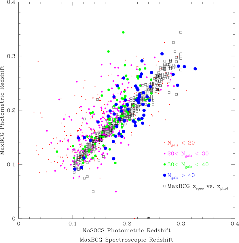
Figure 12.— Left: Comparison of NoSOCS and MaxBCG redshifts for clusters matched within 0.75Mpc. The solid circles show the NoSOCS photometric redshifts compared to those from MaxBCG. The point size increases with increasing richness. Open squares show the MaxBCG spectroscopic redshifts vs. their photometric redshifts. Right: The dispersion (top) and median offset (bottom) between NoSOCS and MaxBCG photometric redshifts, as a function of richness and matching radius.

5.3.2 Richness

The number of galaxies in a cluster may be directly related to the underlying dark halo mass. If this is true, purely photometric cluster surveys are adequate to construct the cluster mass function, and in concert with photometric redshifts, measure its evolution.

To test the reliability of such richness estimates, we compare our richnesses to those from the MaxBCG catalog. Both surveys compute richnesses in fixed physical apertures as well as within $r_{200}$. The results are show in Figure 13, where the left panel shows our $N_{gals}$ (within a 500kpc radius aperture) versus MaxBCG richnesses in the same aperture, and the right panel compares our fixed-aperture richness with MaxBCG’s $R_{200}$ richness. We only use clusters whose centroids agree to within 500 $h^{-1}$ kpc between the two surveys, and with $0.1<z_{phot}<0.3$, resulting in a sample of 1,072 clusters. The small blue points show all matched clusters, while red points are those matches where the NoSOCS and MaxBCG photometric redshifts differ by less than 0.03. The large open squares show the medians in bins of width $\Delta N_{gals}=10$, along with the rms scatter. Although there is a moderately large dispersion between our richnesses and those from MaxBCG, they are well correlated. The solid lines in Figure 13 show the best-fit relations:

$${N_{gals,MaxBCG}=12.55+0.260\times N_{gals}}$$ (6)

and

$${N_{R200,MaxBCG}=8.60+0.375\times N_{gals}}$$ (7)

As expected, the richnesses computed within the same fixed apertures (0.5 Mpc) are much better correlated. However, these relations should not be used to convert between richnesses from the two surveys. The MaxBCG catalog is censored at low richness (where most of the clusters are found) and the scatter in the relation is very high. Much of the scatter is likely due to the different definitions of richness, where we count all galaxies while MaxBCG effectively counts only galaxies along the E/S0 ridgeline. Due to the large photometric errors in DPOSS, we cannot replicate a richness using only the red-sequence galaxies. Additional scatter is introduced by the different photometric redshifts changing the angular sizes of the apertures between the two surveys.

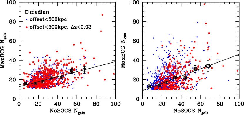
Figure 13.— Comparison of NoSOCS and MaxBCG richnesses for clusters with $0.1<z_{phot}<0.3$ matched within 0.5Mpc. Small blue points show all of these clusters, while larger red points require that the photometric redshifts agree within $\Delta z<0.03$. Large square show the medians in bins of width $\Delta N_{gals}=10$. The left panel compares richnesses measured in the same fixed aperture of 500 kpc. The right panel compares our fixed-aperture richness with the MaxBCG richness within their $R_{200}$. The best fit relations are shown as the solid lines.

6. X-ray Measurements

6.1. Comparison to NORAS

It is instructive to compare the results of optical and X-ray cluster surveys, for the purposes of examining completeness and testing properties ($N_{gals},L_{X},L_{opt}$) that might be useful as mass proxies. The largest existing X-ray survey in the Northern hemisphere is NORAS (Böhringer et al., 2000), with 378 clusters at $\delta>0^{\circ}$. NORAS is useful not only as the largest, homogeneous catalog of low-to-moderate redshift clusters, but also because spectroscopic redshifts have been obtained for the entire sample. To match this sample to NoSOCS, we first remove 55 NORAS clusters in our bad areas, and an additional 97 at low galactic latitude. This leaves a sample of 226 NORAS clusters for comparison, of which 175 are at $0.05<z<0.3$, where we expect NoSOCS to be very complete.

Figure 14.— NoSOCS photometric redshifts vs. NORAS spectroscopic redshifts. Points are color coded by the closeness of the positional match.

The top panels of Figure 15 show the recovery rate of X-ray selected clusters by our survey as a function of NORAS spectroscopic redshift (left) and X-ray luminosity (right, for clusters with $0.05<z_{NORAS}<0.3$). At $0.05<z<0.3$ we recover 80-95% of the NORAS clusters, depending on the matching radius, with a distinct drop at $z>0.25$, as expected from our completeness functions. At high $L_{X}$, we recover 100% of the NORAS clusters, but they are few in number. At moderate $L_{X}$ ($\sim 10^{45}$ erg s^-1), the recovery rate is quite stable near 80%, mostly due to clusters missed at higher redshifts. The bottom panels show the reverse comparison, the recovery rate of optical clusters, as a function of NoSOCS photometric redshift (left) and optical richness (right). As with other optical cluster surveys, we have nearly two orders of magnitude more candidates than NORAS, resulting in a very low recovery rate of NoSOCS clusters in the X-ray. The recovery rate increases with redshift, as the fraction of poor clusters decreases in the optical. This effect is clearly illustrated in the bottom right panel, as the recovery rate approaches 50% for clusters with $N_{gals}>80$. Nevertheless, it appears that NORAS misses over half of the richest clusters in our sample. The extensive spectroscopy for NORAS also allows an additional check on our photometric redshifts. The left panel of Figure 14 plots NoSOCS $z_{phot}$ against NORAS $z_{spec}$, with matches within 0.5$h^{-1}$ Mpc shown in black, $0.5<{\rm offset}<0.75h^{-1}$ Mpc in green, and $0.75<{\rm offset}<1.0h^{-1}$ Mpc in red. For the 145 clusters matched within 0.5$h^{-1}$ Mpc, we find $Q_{\sigma}(z_{NoSOCS,phot}-z_{NORAS,spec})/(1+z_{NORAS,spec})=\mathrm{\Delta}z=0.026$, consistent with the errors estimated from the photometric relation combined in quadrature with the background estimation errors. The recovery rates and typical offsets are also in good agreement with Lopes et al. (2006), who compared NoSOCS clusters to the more heterogeneous BAX database.

Figure 15.— Top Left: NoSOCS recovery rate of NORAS clusters as f($z_{NORAS}$). Top Right: NoSOCS recovery rate of NORAS clusters as f($L_{X}$), for clusters with $0.05<z_{NORAS}<0.3$. Bottom Left: NORAS recovery rate of NoSOCS clusters as f($z_{phot}$). Bottom Right: NORAS recovery rate of NoSOCS clusters as f($N_{gals}$).

6.2. X-ray Luminosities from RASS

As seen in Figure 14, X-ray measurements from NORAS are only available for a very small fraction of optically selected clusters. However, one can use the locations of optically selected cluster candidates to measure X-ray fluxes and luminosities from RASS, allowing us to improve the optical–X-ray correlations. Even though the significance of X-ray emission in these areas may be too low to identify extended sources in RASS, we can derive either fluxes or upper limits following Böhringer et al. (2000) to generate a much larger dataset.

We first restrict the NoSOCS sample to clusters at $0.069\leq z_{phot}\leq 0.196$, the same redshift range used for substructure measurement. The optical richnesses are most reliable at these distances, where the luminosity function is completely sampled over the magnitude range used to derive $N_{gals}$. We further restrict the sample to clusters with $N_{gals}\geq 25$, as we do for measuring $R_{200}$, to avoid poor clusters/groups where the X-ray emission is unlikely to be detected or may be dominated by the X-ray halo of a single galaxy. The X-ray luminosities $L_{X}$ are estimated from count rates in ROSAT PSPC images taken as part of the RASS. Images and exposure maps in the 0.4-2.4 keV band are retrieved from the ROSAT archive via FTP. We avoid the softest ROSAT channels (0.1-0.4 keV) since the background is higher. To make our measurements comparable to those of Böhringer et al. (2000), we follow an almost identical procedure. The background is estimated in an annulus with an inner radius of $20^{\prime}$ and width of $21.3^{\prime}$, divided into twelve sectors. The median count rate from these sectors is used as the background, after removing any sectors containing point sources. The details of this procedure are described in §3.1 of Böhringer et al. (2000). The cluster X-ray flux is then computed using fixed apertures of 0.5 and 1.0 $h^{-1}$ Mpc radius. We do not perform the growth curve analysis (GCA) because the vast majority of NoSOCS clusters have very low X-ray fluxes, making the GCA extremely unstable. The computed X-ray fluxes are then corrected for flux missing from the faint outer regions using the technique described in §3.5 of Böhringer et al. (2000). Finally, only clusters whose total counts are $3\sigma$ above the background are considered reliable. All others are reported as upper limits. The X-ray luminosities measured within fixed apertures of 0.5 and 1.0 $h^{-1}$ Mpc (in units of 10⁴³ erg s^-1) along with the associated errors and X-ray temperatures (in keV) can be found in Table 5. Column 1 gives the cluster name, while Columns 2-4 give the X-ray luminosity, luminosity error, and temperature, all derived within a 0.5 $h^{-1}$ Mpc aperture. Columns 5-7 provide the same quantities measured using a 1.0 $h^{-1}$ Mpc aperture. Luminosities marked with a “:” are upper limits.

6.2.1 Validation with NORAS and REFLEX

To test our methodology, we have recomputed $L_{X}$ for the entire NORAS and REFLEX (Böhringer et al., 2001) samples using our software. We use the GCA-derived apertures reported in those two surveys, along with the redshifts, missing flux corrections and plasma models taken directly from the respective samples. Rather than transform between the different cosmologies used in NORAS and REFLEX, we perform all calculations with the cosmological parameters used in those surveys. To convert the measured total count rate to an unabsorbed X-ray flux in the full ROSAT soft energy band (0.1 - 2.4 keV), we use the PIMMS tool available through NASA HEASARC. We assume a Raymond-Smith (RS) spectrum (Raymond & Smith, 1977) to represent the hot plasma present in the intracluster medium, with a metallicity of 0.2 of the solar value and the interstellar hydrogen column density along the line-of-sight taken from Kalberla et al. (2005) and Bajaja et al. (2005). The plasma temperature is estimated in two different ways. First, we use a fixed temperature of 5 keV, which is typical for clusters (Markevitch, 1998), and term the resulting luminosity $L_{X5}$. Second, we use an iterative procedure relying on the $L_{X}-T_{X}$ relation from Markevitch (1998). We start by calculating $L_{X5}$ and finding the corresponding temperature, assuming an RS spectrum. This new temperature is used to recalculate the luminosity based on an RS spectrum, and the procedure is iterated until convergence is reached, when the change in temperature is $\Delta T_{X}<1keV$, comparable to the scatter in the $L_{X}-T_{X}$ relation. The procedure typically converges in two or three iterations. For both luminosity measures, we apply a $K$-correction (Böhringer et al., 2000) to derive the X-ray luminosity in the rest frame 0.1 - 2.4 keV band.

The only significant methodological differences between our technique and the previously published works are (i) we use the 0.4-2.4 keV images provided by the ROSAT archive, while they worked directly from the event files in the 0.5-2 keV range, (ii) we use a metallicity of $0.2Z_{\odot}$ instead of $0.3Z_{\odot}$, and (iii) they derive an independent count rate to flux conversion while we rely on PIMMS. Nevertheless, our results are in excellent agreement with both surveys. The comparisons to NORAS and REFLEX are shown in the top and bottom panels of Fig. 16, respectively. We find very small offsets of $\sim 5\%$ in $L_{X}$ between our measurements and the literature values, likely due to differences in the count rate to flux conversion. The scatter is small, $\sigma(\delta LogL_{x})\sim 0.03$ over a very broad range of $L_{X}$, demonstrating that we are able to correctly recover X-ray luminosities with our technique.

Figure 16.— Comparison of X-ray luminosities computed using our methodology vs. NORAS (left) and REFLEX (right) .

Four examples of the optical and X-ray properties are shown in Figure 17, where we overlay contours of X-ray emission from the RASS on DPOSS $F$-band images of four clusters in our catalog. The images are 0.5^∘ on a side, centered on the NoSOCS optically-selected cluster centers. The clusters range in richness from $N_{gal}=30-90$, and redshifts of $z=0.07-0.183$. There are 6 X-ray contours evenly spaced between the background level and $2\sigma$ over the background. A circle of radius $0.5\times R_{Abell}$ is plotted, centered on the X-ray flux centroid. Although evident in the optical images, the X-ray fluxes are clearly not very high, and even moderately rich clusters near the median redshift of our catalog (such as the one at top right in the figure) do not stand out strongly. The X-ray contours are usually well matched to the optical center, except for the top left cluster. Visual inspection of the galaxy distribution in the latter field shows that the NoSOCS cluster center is in between two apparent overdensities which have been blended in our catalog, and only one of which is X-ray detected. This suggests that searching for clusters with highly discrepant optical and X-ray positions and/or fluxes can be used to find such projections.

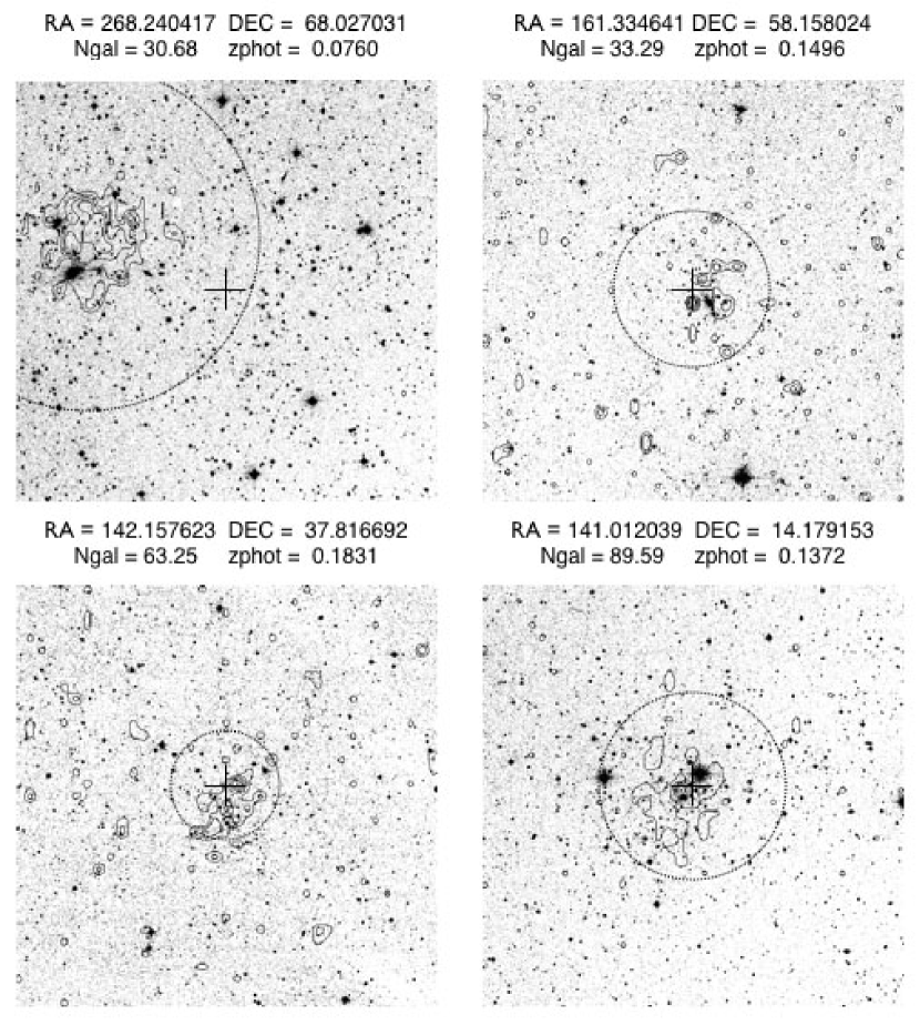
Figure 17.— Contours of X-ray emission from the RASS overlaid on DPOSS $F$-band images of four clusters in our catalog. The images are 0.5^∘ on a side, centered on the NoSOCS optical cluster centers. There are 6 X-ray contours evenly spaced between the background level and $2\sigma$ over the background. A circle of radius $0.5\times R_{Abell}$ is plotted at the X-ray flux centroid, while the optical center is marked with a cross.

6.2.2 Optical vs. X-ray Properties

The comparison of optical richness and our estimate of $L_{X}$ from the iterative procedure described above is shown in Figure 18, using 1649 clusters with $0.07<z<0.19$, $N_{gal}>25$ and successfully measured X-ray luminosities with $L_{X}>5\times 10^{42}$ ergs s^-1. Clusters where the X-ray luminosity is only an upper limit and those where the background estimation failed are not included. Individual clusters are plotted as dots, while the binned results (with each bin containing 200 clusters) along with their $1\sigma$ scatter are shown as the large points with error bars.

While the scatter is large, the binned relationship agrees with that found by Lopes et al. (2006) using higher quality X-ray data, $L_{X}\propto N_{gal}^{1.616}$. We also show, as the solid line, the relationship between $L_{X}$ within 750 kpc and $N_{200}$ from the X-ray stacking analysis performed by Rykoff et al. (2008) using the MaxBCG cluster catalog (their equation 5), but simply replacing $N_{200}$ with our $N_{gals}$. The power-law slopes of the Lopes et al. (2006) and Rykoff et al. (2008) relations are nearly identical, despite the completely different richness measures. As seen in Figure 18, a similar relationship holds for our clusters, despite ROSAT’s limited spatial resolution and count rate as well as the limited photometric accuracy and depth of DPOSS, demonstrating that a reliable cluster sample can be defined from such data. It is also possible transform our $N_{gals}$ to the MaxBCG $N_{200}$ using Eqn. 7, and plot the relation from Rykoff et al. (2008) using this pseudo-$N_{200}$; this is shown as the dashed line in Figure 18. We caution that this is not a reliable conversion because the richness transformation is difficult and Rykoff et al. (2008) use a completely different prescription for computing $L_{X}$.

Table 5X-ray Measurements

	Within $0.5h^{-1}_{70}$ Mpc			Within $1.0h^{-1}_{70}$ Mpc
Name	$L_{X}$ ($10^{43}$ erg s-1)	Err($L_{X}$)	$T_{X}$ (keV)	$L_{X}$ ($10^{43}$ erg s-1)	Err($L_{X}$)	$T_{X}$ (keV)
NSC J111750+685910	0.620	0.140	0.8	0.160:	0.260	0.4
NSC J162305+653454	0.200:	0.960	0.4	1.160	0.510	1.1
NSC J091711+524442	2.120	0.600	1.4	28.760	0.220	5.3
NSC J102307+520201	1.360	0.830	1.2	5.020	0.310	2.2
NSC J101218+460643	1.780	0.520	1.3	1.020	0.380	1.0
NSC J103805+420426	0.160	0.030	0.4	0.160:	0.620	0.4
NSC J173315+374215	0.360	2.450	0.6	5.160	1.320	2.3
NSC J151120+363421	1.590	0.950	1.2	0.860	0.910	0.9
NSC J082043+301238	0.120:	0.000	0.3	1.050	0.160	1.0
NSC J152111+292632	0.370	1.920	0.6	2.900	1.000	1.7
NSC J081942+264129	0.020:	0.090	0.2	3.190	0.040	1.8
NSC J155312+273835	0.570	1.370	0.7	1.820	1.370	1.3
NSC J020211+190446	5.700	0.250	2.4	8.510	0.290	2.9
NSC J114047+181932	4.350	0.580	2.1	2.060	0.600	1.4
NSC J164837+193606	0.270	0.610	0.5	0.280:	0.530	0.5
NSC J085246+161920	0.800	2.300	0.9	1.010:	2.680	1.0
NSC J141229+140110	4.480	0.630	2.1	6.560	0.520	2.5
NSC J011144+100349	0.210	0.120	0.5	1.700	1.430	1.3
NSC J094338+085430	0.190	2.010	0.4	1.920	1.540	1.4
NSC J135224+092048	0.520	0.030	0.7	4.010	0.060	2.0
NSC J021010+080844	0.690	1.450	0.8	5.850	1.370	2.4
NSC J104929+033846	1.770	0.800	1.3	2.530	0.700	1.6
NSC J154555+030814	0.930	0.030	1.0	0.640:	0.260	0.8
NSC J014426+021221	0.570	0.050	0.7	1.850	0.040	1.3
NSC J104534-002506	0.180:	0.460	0.4	0.450:	0.050	0.7
NSC J152156+013000	0.240:	0.000	0.5	1.870	0.060	1.4

While the X-ray data from RASS is limited, especially for the poorer, lower mass systems, this catalog of individual cluster X-ray measurements is the largest compiled to date. It is only recently that astronomers have undertaken systematic comparisons of optical and X-ray cluster samples by returning to the source data and re-extracting physical properties consistently, rather than simply matching catalogs. For instance,Donahue et al. (2002) compared independently detected X-ray and optical clusters from the same patches of sky. They found poor correlation between optical richness and X-ray luminosity, but could not pinpoint the physical reason for this, and pointed out the need to understand the effect of this scatter on mass selection. The RASS-SDSS clusters survey (Popesso et al., 2004) instead uses a small but very well measured sample of 114 X-ray detected clusters, and finds good correlation between X-ray luminosity or temperature and optical luminosity, if one has excellent data and chooses the measurement parameters (such as the aperture for richness measurement) carefully. However, it is worth noting that their sample remains one requiring X-ray detections, which was shown by Donahue et al. (2002) to potentially bias the results.

Figure 18.— Comparison of optical richness $N_{gal}$ and X-ray luminosity $L_{X}$ within 0.5 $h^{-1}$ Mpc for 1649 clusters with $0.07<z<0.19$, $N_{gal}>25$ and $L_{X}>5\times 10^{42}$ ergs s^-1. Individual clusters are plotted as dots, while the binned results (with each bin containing 200 clusters) along with their rms errors shown as the large squares with error bars. The solid line shows the relation $L_{X,750kpc}=e^{3.4}(\frac{N}{40})^{1.61}$ found by Rykoff et al. (2008), directly replacing their $N_{200}$ with our $N_{gals}$. The dashed line shows the same relation, but now transforming our $N_{gals}$ to MaxBCG $N_{200}$ using Eqn. 7. Dotted lines show the $N_{gal}>25$ limit for attempting to measure $L_{X}$ and the $L_{X}>5\times 10^{42}$ ergs s^-1 limit imposed on the sample when computing binned medians.

The only other large optical - X-ray comparisons are those of Dai et al. (2007), who used stacking techniques to derive X-ray properties of over 4000 clusters selected optically from the Two-Micron All Sky Survey (2MASS), and Rykoff et al. (2008), who stacked X-ray data for $\sim 17,000$ MaxBCG clusters from the SDSS. Even with the low redshift limit ($z<0.1$) imposed by the shallow depth of 2MASS, Dai et al. (2007) relied on stacking of X-ray data for clusters binned by their optical properties to measure correlations between mass (optical richness), luminosity and temperature. They find similar correlations to those in the literature for individual clusters, but must model the Poisson fluctuations in the number of galaxies in a cluster of a given mass. At higher redshifts, where evolution in the cluster populations becomes more important, understanding and modeling these fluctuations will be more challenging. Rykoff et al. (2008) were able to examine some issues related to bias arising from scatter in the $L_{X}$-richness relation with a small sample of clusters where individual X-ray measurements were possible.

7. Conclusions

We have presented NoSOCS, a new cluster catalog based on the $|b|>30^{\circ}$ plate scans from the Digitized Second Palomar Observatory Survey. Spanning over $\pi$ steradians, this is the largest area optical cluster catalog created since those of Abell (1958) and Abell, Corwin & Olowin (1989). In terms of area coverage, it will only be superseded by new sky surveys such as Pan-STARRS (Kaiser, 2004) and LSST (Tyson, 2006), both of which have cosmology through clusters as important science drivers. We show consistency among the three regions covered by NoSOCS, and with the SDSS MaxBCG cluster catalog of Koester et al. (2007b). However, interesting discrepancies between these two large surveys remain. These include large numbers of poor clusters missed by one survey but found in another, suggesting lower completeness, higher contamination, or some combination of the two for such systems, in either or both surveys. Even for supposedly rich clusters there are sufficient discrepancies to call into question our ability to use such surveys for high-precision cosmological constraints. Understanding the sources of these disagreements requires further investigation of both systematic errors and individual cluster candidates.

We have also derived X-ray luminosities for a large subset of our cluster sample from ROSAT all-sky X-ray survey data. We demonstrate that the optical richness and X-ray luminosities are well correlated, albeit with moderate scatter. We find that, despite the poor photometric data and low X-ray luminosities of most NoSOCS clusters, the correlation between $L_{x}$ and $N_{gals}$ is in good agreement with literature results using better data and stacking analyses. Refinements to both the optical richnesses and especially deeper X-ray survey data will be necessary to improve this relation and truly understand the utility of optical richnesses for mass estimation. Nevertheless, our results show promise for using large surveys for such measurements in cases where the data quality is less than superb, as may be expected for the highest redshift clusters even in upcoming deep surveys such as Pan-STARRS and LSST. Furthermore, our ability to measure X-ray luminosities for hundreds of clusters not originally detected in the RASS argues for improved multi-wavelength detection methods that leverage multiple surveys (optical, infrared, X-ray, S-Z) to find distant and/or poor clusters which would otherwise fall below the significance cutoff in a single passband.

References

- Abell (1958) Abell, G. O. 1958, ApJS, 3, 211
- Abell, Corwin & Olowin (1989) Abell, G. O., Corwin, H. G. & Olowin, R. P. 1989, ApJS, 70, 1
- Adelman-McCarthy et al. (2007) Adelman-McCarthy, J. K., et al. 2007, ApJS, 172, 634
- Andernach & Coziol (2006) Andernach, H., & Coziol, R. 2006, ArXiv Astrophysics e-prints, arXiv:astro-ph/0603295
- Bahcall et al. (2003) Bahcall, N. A. et al. 2003, ApJS, 148, 243
- Bajaja et al. (2005) Bajaja, E., Arnal, E. M., Larrarte, J. J., Morras, R., Pöppel, W. G. L., & Kalberla, P. M. W. 2005, A&A, 440, 767
- Baum (1959) Baum, W. A. 1959, PASP, 71, 106
- Bertin & Arnouts (1996) Bertin, E. & Arnouts, S. 1996, A&AS, 117, 393
- Blanton et al. (2001) Blanton, M. R., et al. 2001, AJ, 121, 2358
- Blanton et al. (2005) Blanton, M. R., Eisenstein, D., Hogg, D. W., Schlegel, D. J., & Brinkmann, J. 2005, ApJ, 629, 143
- Bloom et al. (2006) Bloom, J. S., et al. 2006, ApJ, 638, 354
- Böhringer et al. (2000) Böhringer, H. et al. 2000, ApJS, 129, 435
- Böhringer et al. (2001) Böhringer, H., et al. 2001, A&A, 369, 826
- Bower et al. (1992) Bower, R. G., Lucey, J. R., & Ellis, R. S. 1992, MNRAS, 254, 589
- Carlberg et al. (1997) Carlberg, R. G., et al. 1997, ApJ, 485, L13
- Collister & Lahav (2005) Collister, A. A., & Lahav, O. 2005, MNRAS, 361, 415
- Courtois et al. (2004) Courtois, H., Paturel, G., Sousbie, T., & Sylos Labini, F. 2004, A&A, 423, 27
- Dai et al. (2007) Dai, X., Kochanek, C. S., & Morgan, N. D. 2007, ApJ, 658, 917
- de Carvalho et al. (2005) de Carvalho, R. R., Gonçalves, T. S., Iovino, A., Kohl-Moreira, J. L., Gal, R. R., & Djorgovski, S. G. 2005, AJ, 130, 425
- de Vaucouleurs et al. (1991) de Vaucouleurs, G., de Vaucouleurs, A., Corwin, H. G., Jr., Buta, R. J., Paturel, G., & Fouque, P. 1991, Springer-Verlag: Berlin
- Djorgovski et al. (1999) Djorgovski, S. G., Gal, R. R., Odewahn, S. C., de Carvalho, R. R., Brunner, R., Longo, G., & Scaramella, R. 1999, in ”Wide Field Surveys in Cosmology”, eds. S. Colombi, Y. Mellier, & B. Raban, Gif sur Yvette: Editions Frontieres, p. 89.
- Donahue et al. (2002) Donahue, M., et al. 2002, ApJ, 569, 689
- Dressler (1980) Dressler, A. 1980, ApJ, 236, 351
- Frith et al. (2003) Frith, W. J., Busswell, G. S., Fong, R., Metcalfe, N., & Shanks, T. 2003, MNRAS, 345, 1049
- Gal et al. (2000) Gal, R. R., de Carvalho, R. R., Odewahn, S. C., Djorgovski, S. G. & Margoniner, V. E. 2000, AJ, 119, 12
- Gal et al. (2003) Gal, R. R., de Carvalho, R. R., Lopes, P. A. A., Djorgovski, S. G. Brunner, R. R. & Odewahn, S. C. 2003, AJ, 125, 2064
- Gal et al. (2004) Gal, R. R., de Carvalho, R. R., Odewahn, S. C., Djorgovski, S. G., Mahabal, A., Brunner, R. J., & Lopes, P. A. A. 2004, AJ, 128, 3082
- Gal (2008) Gal, R. R. 2008 in A Pan-Chromatic View of Clusters of Galaxies and the Large-Scale Structure, ed. Plionis, M, López-Cruz, O. and Hughes, D. Lecture Notes in Physics, Berlin Springer Verlag, 119
- Gehrels et al. (2005) Gehrels, N., et al. 2005, Nature, 437, 851
- Gladders & Yee (2000) Gladders, M. D., & Yee, H. K. C. 2000, AJ, 120, 2148
- Gunn & Gott (1972) Gunn, J. E., & Gott, J. R. I. 1972, ApJ, 176, 1
- Hansen et al. (2005) Hansen, S. M., McKay, T. A., Wechsler, R. H., Annis, J., Sheldon, E. S., & Kimball, A. 2005, ApJ, 633, 122
- Hennawi et al. (2008) Hennawi, J. F., et al. 2008, AJ, 135, 66
- Kaiser (2004) Kaiser, N. 2004, Proc. SPIE, 5489, 11
- Kalberla et al. (2005) Kalberla, P. M. W., Burton, W. B., Hartmann, D., Arnal, E. M., Bajaja, E., Morras, R., Pöppel, W. G. L. 2005, A&A, 440, 775
- Koester et al. (2007a) Koester, B. P., et al. 2007, ApJ, 660, 221
- Koester et al. (2007b) Koester, B. P., et al. 2007, ApJ, 660, 23
- Lin et al. (2004) Lin, Y.-T., Mohr, J. J., & Stanford, S. A. 2004, ApJ, 610, 745
- Lopes et al. (2004) Lopes, P. A. A., de Carvalho, R. R., Gal, R. R., Djorgovski, S. G., Odewahn, S. C., Mahabal, A. A., & Brunner, R. J. 2004, AJ, 128, 1017
- Lopes et al. (2006) Lopes, P. A. A., de Carvalho, R. R., Capelato, H. V., Gal, R. R., Djorgovski, S. G., Brunner, R. J., Odewahn, S. C., & Mahabal, A. A. 2006, ApJ, 648, 209
- Lopes et al. (2008) Lopes, P. A. A., de Carvalho, R. R., Kohl-Moreira, J. L., & Jones, C. 2008, MNRAS, 1356
- Markevitch (1998) Markevitch, M. 1998, ApJ, 504, 27
- Odewahn et al. (2004) Odewahn, S. C., et al. 2004, AJ, 128, 3092
- Paolillo et al. (2001) Paolillo, M., Andreon, S., Longo, G., Puddu, E., Gal, R. R., Scaramella, R., Djorgovski, S. G., & de Carvalho, R. 2001, A&A, 367, 59
- Pinkney et al. (1996) Pinkney, J., Roettiger, K., Burns, J., Bird, C. 1996, ApJS, 104, 1
- Popesso et al. (2004) Popesso, P., Böhringer, H., Brinkmann, J., Voges, W., & York, D. G. 2004, A&A, 423, 449
- Popesso et al. (2007) Popesso, P., Biviano, A., Böhringer, H., & Romaniello, M. 2007, A&A, 464, 451
- Postman, Lauer, Oegerle, & Donahue (2002) Postman, M., Lauer, T. R., Oegerle, W., & Donahue, M. 2002, ApJ, 579, 93
- Raymond & Smith (1977) Raymond, J. C., & Smith, B. W. 1977, ApJS, 35, 419
- Rozo et al. (2007) Rozo, E., Wechsler, R. H., Koester, B. P., Evrard, A. E., & McKay, T. A. 2007, ArXiv Astrophysics e-prints, arXiv:astro-ph/0703574
- Rykoff et al. (2008) Rykoff, E. S., et al. 2008, ApJ, 675, 110
- Silverman (1986) Silverman, B. W. 1986, Monographs on Statistics and Applied Probability, London: Chapman and Hall
- Struble & Rood (1991) Struble, M. F., & Rood, H. J. 1991, ApJS, 77, 363
- Tyson (2006) Tyson, J. A. 2006, Intersections of Particle and Nuclear Physics: 9th Conference CIPAN2006, 870, 44
- Yee & Ellingson (2003) Yee, H. K. C., & Ellingson, E. 2003, ApJ, 585, 215
- York et al. (2000) York, D. G. et al. 2000, AJ, 120, 1579