Parallelization of Markov Chain Generation and its Application to the Multicanonical Method

Abstract

We develop a simple algorithm to parallelize generation processes of Markov chains. In this algorithm, multiple Markov chains are generated in parallel and jointed together to make a longer Markov chain. The joints between the constituent Markov chains are processed using the detailed balance. We apply the parallelization algorithm to multicanonical calculations of the two-dimensional Ising model and demonstrate accurate estimation of multicanonical weights.

, , and

1 Introduction

The MCMC (Markov Chain Monte-Carlo) method [1] has played an important role in study of complex systems with many degrees of freedom. For example, MCMC has been applied to various many-body problems such as proteins [2], spin systems [3], and lattice gauge theory [4]. Although the method has achieved great success, there are systems where Monte-Carlo sampling does not work due to local minima of energy functions. For example, in analysis of protein folding, Monte-Carlo random walks are trapped in narrow regions of energy space because there are so many local minima. For large proteins, it is a hard problem to obtain sufficiently large number of statistical samples because it takes very long time for a complicated conformation to escape from a local minimum in energy space.

The multicanonical method [5, 6, 7] may be useful for resolving the local minimum problems. It is a kind of generalized-ensemble methods. It has been applied to the above mentioned problems and worked nicely. Especially its application to protein folding with the multicanonical MD [8, 9] has been remarkable. Recently, Ikebe et al have succeeded in folding calculation of a 40-residue protein [10]. Kamiya et al have demonstrated flexible molecular docking between a protein and a ligand [11]. Since protein structure prediction is one of the most important subjects in life sciences, it has been expected that the multicanonical method will make a large progress in clarification of the fundamental laws of life and development of high-performance drugs.

The multicanonical method is based on an artificial ensemble that gives a flat probability distribution in energy space. The advantage of the method is enhancement of rare configurations, which results in random walks in wide range of energy space. In this method, multicanonical weights are estimated in an iterative way. To estimate a multicanonical weight, one has to generate a Markov chain many times, which must be sufficiently long for accurate estimation. The number of arithmetic operations increases exponentially as the number of amino-acid residues becomes large. Since actual proteins are composed of more than a hundred amino-acid residues, the number of necessary operations for folding simulation is huge. It would be a possibility to decrease the execution time using massively parallel supercomputers.

In this paper, we propose an algorithm to generate a Markov chain in a parallel way. In MCMC calculations, the detailed balance is checked between the last and a newly generated configuration to determine acceptance or rejection of the new one. Accepted configurations constitute a so-called Markov chain. A Markov chain is a one-dimensional object that is generated serially. Since acceptance or rejection of a new configuration depends on the last configuration, naive algorithm for Markov-chain generation such as the Metropolis method is essentially serial. At a glance, it seems that the MCMC algorithm cannot be parallelized. In this paper, we are going to show a method to joint multiple Markov chains together to make a longer Markov chain. The constituent Markov chains are independently generated starting from different initial configurations. The essential point of the method is that joints between chains are processed so that the detailed balance is satisfied. Based on the detailed balance, unnecessary configurations are discarded from each Markov chain. The remaining Markov chains are connected together to make a longer Markov chain. By repeating this procedure, one can increase the length of the Markov chain arbitrarily. In this algorithm, other operations such as evaluation of energy functions are not parallelized.

To demonstrate how the parallelization algorithm works, we solve the two-dimensional Ising model by combining the proposed parallelization algorithm and the multicanonical method. Multicanonical weights are estimated from histograms, which are obtained using the parallelization algorithm.

In Sec. 2, we introduce an algorithm to generate a long Markov chain in a parallel way. In Sec. 3, we review the multicanonical method briefly. In Sec. 4, we apply the parallelization algorithm to the two-dimensional Ising model with the multicanonical method. In Sec. 5, we show numerical results. Sec. 6 is devoted to conclusions.

2 Parallelization of Markov-Chain Generation

Let us consider a Markov chain that is composed of $M$ configurations,

$$C_{1},C_{2},\dots,C_{M}.$$ (2.1)

We call $C_{k}$ a configuration, which is a set of values of multiple variables. $C_{k}$ are generated so that configurations distribute according to a specified probability distribution $P(C)$. In actual calculations, the number of configurations is finite. Therefore, a set of configurations only reproduces $P(C)$ approximately. The associated errors vanishes in the limit $M\to\infty$.

In MCMC, configurations are generated serially so that the detailed balance is satisfied. One determines acceptance or rejection of a randomly generated configuration $C_{k}$ by checking the detailed balance between $C_{k-1}$ and $C_{k}$. At a glance, the MCMC algorithm seems to be essentially serial and is not suited to parallel computation. In order to decrease execution time using parallel computers, we propose a simple algorithm to parallelize Markov-chain generation.

Let us consider a computer of which parallelism is $p$. In our parallelization algorithm, each computing node generates a Markov-chain separately. In order to obtain a much longer Markov chain having $M_{\rm total}$ configurations than a Markov chain having $M_{\rm node}$ configurations generated by each computing node, the $p$ Markov chains are connected satisfying the detailed balance condition as follows:

Algorithm

1.

Set the total histogram zero, $h(E)=0$, where $E$ is energy variable. Prepare initial configurations $C_{1}^{(i)}$ randomly on $i$-th node ($i=0,\dots,p-1$).

2.

In each node, generate a Markov chain composed of $M_{\rm node}$ configurations,

$$C_{1}^{(i)}\to C_{2}^{(i)}\to\cdots C_{M_{\rm node}}^{(i)},\quad i=0,\dots,p-1.$$ (2.2)

3.

Set $i=0$.

4.

In the $i$-th node, check the detailed balance between $C_{M_{\rm node}}^{(n)}$ and $C_{k}^{(i)}$, where $C_{M_{\rm node}}^{(n)}$ with $n=(i-1+p)$ mod $p$ is the last configuration of the previous node. The index $k$ is increased from $1$ to $M_{\rm node}$ till the detailed balance is satisfied. When there is a configuration that satisfies the detailed balance, that configuration and the succeeding ones are accepted. When there is no accepted configuration, set $C_{M_{\rm node}}^{(i)}\leftarrow C_{M_{\rm node}}^{(n)}$. Make a local histogram $h_{\rm local}(E)$ using only the accepted configurations. Calculate the total histogram, $h(E)\leftarrow h(E)+h_{\rm local}(E)$. Send the values of $h(E)$ and the energy of $C_{M_{\rm node}}^{(i)}$ to the $((i+1)\;{\rm mod}\;p)$-th node. (When $i=0$, $C_{M_{\rm node}}^{(p-1)}$ of the previous iteration is used for checking of the detailed balance.)

5.

Set $i\leftarrow i+1$. If $i<p$, go to step 4.

6.

If the total number of the configurations contained in the total histogram $h(E)$ is smaller than the specified value $M_{\rm total}$, adjust $M_{\rm node}$ appropriately so that additional calculations are minimized, and then go to step 2.

We are going to give some remarks on the algorithm below.

The algorithm produces a Markov chain of which the configuration number is $M_{\rm total}$. Actually, the algorithm outputs the total histogram $h(E)$. As shown in the next section, the obtained histogram $h(E)$ is used to estimate a multicanonical weight $w(E)$. The algorithm is repeated certain times till a multicanonical weight that covers a sufficiently large energy area is obtained. Since the algorithm only assumes the detailed balance and does not depend on the details of probability distribution, the algorithm works in any MCMC calculations.

In each node, the last configuration generated in the previous iteration is used for generating a Markov chain as an initial configuration in the next iteration including when the considered weight has been updated. This means that $p$ Markov chains are generated independently from first to last. Equilibrium depends on the current weight.

There may be no configuration that satisfies the detailed balance in step 4. In this case, all of the configurations contained in that computing node is discarded, which results in low efficiency of Markov-chain generation. One can increase acceptance rate by ordering computing nodes according to energy values of generated configurations. We will pursue this technique in the next paper.

3 The Multicanonical Method

3.1 Estimation of Multicanonical Weights

We are going to combine the algorithm introduced in the previous section with the multicanonical method. Let us review the multicanonical method briefly. For the details of the multicanonical method, see [5, 6, 7].

Consider a statistical system that is defined with a Boltzmann weight

$$w_{\rm B}(E)=e^{-\beta E},$$ (3.1)

where $\beta=1/k_{\rm B}T$. Hereafter, we set $k_{\rm B}=1$ for simplicity.

Probability distribution is given by

$$P(E)=c_{\beta}D(E)w_{\rm B}(E),$$ (3.2)

where $D(E)$ is density of states. The constant $c_{\beta}$ is determined with the normalization condition$\sum_{E}P(E)=1$.

In the multicanonical method, an extended weight $w_{\rm M}(E)$ is defined so that multicanonical distribution is independent of energy,

$$P_{\rm M}(E)=c_{\rm M}D(E)w_{\rm M}(E)\sim c_{\rm M}.$$ (3.3)

We can obtain the multicanonical weight $w_{\rm M}$ in a recursive way. We denote the $n$-th multicanonical weight as $w^{(n)}$, where $n=1,2,\dots,I$. In the initial step, we set $w^{(1)}=1$, which corresponds to high-temperature limit of the Boltzmann weight $w_{\rm B}$. With the $w^{(n)}$, we generate a sufficiently long Markov chain and obtain a total histogram $h^{(n)}(E)$. Then, we generate the next weight $w^{(n+1)}$ using the current weight $w^{(n)}$ and the obtained histogram $h^{(n)}(E)$.

$$w^{(n+1)}(E)=\cases{w^{(n)}(E),&if $h^{(n)}(E)=0$,\cr\displaystyle\frac{w^{(n)}(E)}{h^{(n)}(E)},&otherwise.\cr}$$ (3.4)

We expect that the weight $w^{(n)}$ approaches to the correct multicanonical weight $w_{\rm M}$ if this process is repeated certain times.

To obtain the multicanonical weight accurately, sufficiently large statistics are necessary for generating $h^{(n)}(E)$. We can decrease execution time consumed to generate sufficiently long Markov chains by making use of the parallelization algorithm introduced in Sec. 2. [12].

3.2 Evaluation of Statistical Average

We can calculate statistical average at arbitrary temperature with the following reweighting formula:

$$\langle O(x)\rangle\equiv\sum_{x}O(x)P(x)=\frac{\sum_{i}O(x^{(i)})D(E(x^{(i)}))e^{-\beta E(x^{(i)})}}{\sum_{j}D(E(x^{(j)}))e^{-\beta E(x^{(j)})}},$$ (3.5)

where $x$ represents multiple variables and $x^{(i)}$ is a configuration. If the operator $O(x)$ can be represented as a function of energy $E$ and the multicanonical weight $w_{\rm M}(E)$ is known, one can evaluate Eq. (3.5) without configurations. In this case, the formula (3.5) reduces to

$$\langle O(x)\rangle=\frac{\sum_{E}O(E)w_{\rm M}(E)^{-1}e^{-\beta E}}{\sum_{E}w_{\rm M}(E)^{-1}e^{-\beta E}},$$ (3.6)

because the density of states is inversely proportional to the weight ($D(E)\propto 1/w(E)$) and the histogram has flat distribution. In Eq. (3.6), we can evaluate $\langle O(x)\rangle$ by taking the summation for all possible energy values $E$. The reduced reweighing formula (3.6) cannot be used for quantities that are dependent on local variables.

4 Application to the 2D Ising Model

We are going to solve the two-dimensional Ising model at finite temperature combining the parallelization algorithm (Sec. 2) and the multicanonical method (Sec. 3).

4.1 The 2D Ising Model

The model is defined on two dimensional square lattices. The number of lattice sites is $N=L^{2}$, where $L$ is the lattice size. We assume periodic boundary conditions. The Hamiltonian of the model is defined as follows:

$$H=-\sum_{\langle i,j\rangle}s_{i}s_{j},\quad s_{i}=\pm 1,$$ (4.1)

where the summation is taken for all possible nearest-neighbour sites. All information of thermodynamics is contained in the partition function

$$Z=\sum_{s_{1},\dots,s_{N}}e^{-\beta H}.$$ (4.2)

Based on this, we calculate energy $E$, specific heat $C$, free energy $F$, and entropy $S$ in a statistical way.

$$E \equiv \langle H\rangle,$$ (4.3)

$$C \equiv \frac{dE}{dT}=\beta^{2}(\langle H^{2}\rangle-\langle H\rangle^{2}),$$ (4.4)

$$F \equiv -\frac{1}{\beta}\ln Z,$$ (4.5)

$$S \equiv \beta(E-F).$$ (4.6)

4.2 Coding

We apply a combination of the parallelization algorithm and the multicanonical method to the two-dimensional Ising model. We estimate multicanonical weights iteratively with the parallelization algorithm. We implement the codes with FORTRAN77. Our code set is composed of the following two parts: (i) generation of the multicanonical weight and (ii) evaluation of statistical average. These are implemented as separate two codes. Since almost all of the arithmetic operations are contained in the part (i), only the part (i) is parallelized with MPI-1, which is a library specification for message-passing proposed as a standard [15]. The obtained multicanonical weight is used as an input to the part (ii). We calculate statistical average of energy, specific heat, free energy, and entropy. Since these quantities can be represented as functions of energy, we can use the reweighting formula (3.6) in the part (ii). Execution time of the part (ii) is very short like a second on a Xeon 1.50 GHz processor.

We store logarithm of the weight, not the weight itself, because the absolute values of the weight may be very small. For this reason, we perform all necessary operations under logarithm to evaluate statistical quantities.

Each node generates a Markov chain composed of $M_{\rm node}$ samples using the current multicanonical weight. When all $p$ nodes have done Markov-chain generation, the obtained chains are linked together using the detailed balance as explained before. To be concrete, an energy value of the last configuration and the total histogram $h(E)$ are sent to the next node for the detailed-balance checking and histogram generation. The Metropolis method is used for the detailed-balance checking. If the total number of accepted configurations contained in the total histogram $h(E)$ is smaller than the specified sample number $M_{\rm total}$, the chain generation process is repeated. If it is larger than $M_{\rm total}$, the next weight is calculated using Eq. (LABEL:new_weight) and distributed to all the nodes. Then, a new iteration process is started with the new weight. The above iteration process for weight estimation is repeated the specified $I$ times.

5 Numerical Results

With the implemented codes, we generate multicanonical weights using the parallelization algorithm and calculate statistical quantities using Eq. (3.6). Table 1 is a list of parameter values used to plot Fig. 1

Table 1: Parameter values used for calculation of statistical quantities shown in Fig. 1.

Parameter	Value	Meaning
$L$	$100$	Lattice size
$N$	$L^{2}$	The number of lattice sites
$p$	$32$	Parallelism
$M_{\rm total}$	$10^{8}$	The total number of samples for one iteration
$M_{\rm node}$	$M_{\rm total}/p$	The number of samples generated by a node for one iteration
$I$	$1300$	The number of iterations for weight generation

In Fig. 1, we compare our results with the exact finite-lattice ones obtained by Ferdinand and Fisher [16] when lattice size is $L=100$. As shown in figures (a), (c), and (d), our results for energy, free energy, and entropy agree with the exact ones very well. On the other hand, in Fig. 1 (b), basically two results agree but we admit slight difference. In general, specific heat is more sensitive to errors associated with obtained multicanonical weights than energy as seen in the definition of specific heat (4.4).

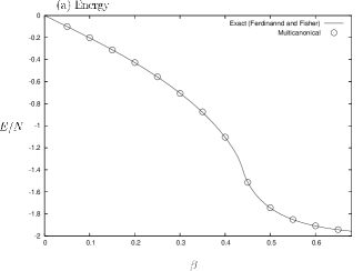
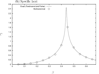
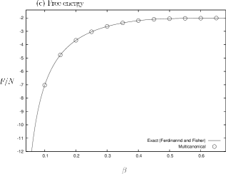
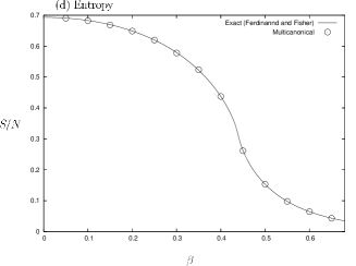
Figure 1: For $L=100$, (a) energy $E/N$, (b) specific heat $C$, (c) free energy $F/N$, and (d) entropy $S/N$ are plotted as functions of inversed temperature $\beta$. The exact results given by Ferdinand and Fisher [16] and ours are plotted with solid lines and circles, respectively.

When parallelism $p$ is small like $1\leq p\leq 1000$, the number of samples generated by each node $M_{\rm node}$ is sufficiently large with a fixed $M_{\rm total}$. In this case, errors associated with multicanonical weights would be small even if the detailed balance is not imposed on the joints of short Markov chains because the number of joints is much smaller than the total number of samples. However, in near future, supercomputers will acquire parallelism of several millions or more. For example, if the same code is executed with $p=10^{6}$ and $M_{\rm total}=10^{8}$, we have $M_{\rm node}=100$, which is quite small. In this case, there are relatively many joints compared to the total number of samples.

In order to confirm that the proposed algorithm works well even when $M_{\rm node}$ is very small, i.e. each constituent Markov chain is very short, we perform a simple experiment. In this experiment, we generate very short Markov chains with $M_{\rm node}=100$, and just connect the chains together without imposing the detailed balance on the joints. This procedure is repeated till the specified number of samples have generated to make a multicanonical weight.

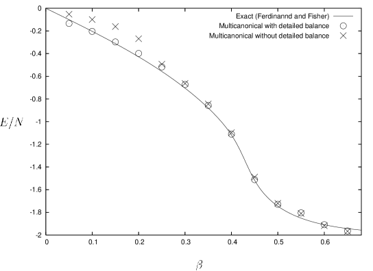
Figure 2: Comparison of energy among the exact (solid line), multicanonical with the detailed balance (circles), and multicanonical without the detailed balance (crosses), where we have set $L=20$, $p=32$, $M_{\rm total}=10^{8}$, and $M_{\rm node}=100$.

Figure 2 is a comparison of energy among three results with $L=20$: exact (solid line), multicanonical with the detailed balance (circles), and multicanonical without the detailed balance (crosses). When the detailed balance is imposed on the joints of constituent Markov chains (circles), the energy agrees well with the exact one. This result is consistent with our intuition because it is in principle guaranteed that sampling based on the detailed balance gives the correct distribution. On the other hand, when the detailed balance is not imposed on the joints (crosses), there is slight deviation of energy from the exact one in the high-temperature region.

According to the reweighting formula (3.6), the low-energy part of the multicanonical weight is dominant when $\beta$ is large. In Fig. 2, the crosses show that the generated weight is sufficiently accurate in the low-energy region. This is because the low-energy part of the weight is generated in the last phase of a weight-generation process and therefore accumulation of errors is not large. On the other hand, the middle-energy part of the weight may accumulate errors because it is updated every iteration with a very short Markov chain that does not cover the entire energy space. This is the cause of the energy deviation for small $\beta$ when the detailed balance is not imposed on joints.

Since even this simple Ising model produces considerable errors for small $M_{\rm node}$, one should be careful when treating more complicated systems. It depends on the shape of the considered multicanonical weight how energy deviates from the true values. When $M_{\rm node}$ is small due to massive parallelism, one can obtain better accuracy by imposing the detailed balance on joints between constituent Markov chains.

Table 2: Execution (E), operation (O), and communication (C) time of the code for parallelism $p=2,4,8,16,32,64$ have been measured with $L=100$ and $M_{\rm total}=10^{8}$ in the first iteration of weight generation. E is the sum of O and C. Scalability of execution time is evaluated in units of the $p=2$ case. A PC cluster with Xeon 1.50 GHz processors has been used for the measurements.

$p$	E (sec)	O (sec)	C (sec)	Scalability
2	12.32	11.77	0.55	2.00
4	6.21	5.93	0.28	3.97
8	3.80	3.59	0.21	6.48
16	2.19	1.66	0.53	11.25
32	1.40	0.77	0.63	17.60
64	0.97	0.43	0.54	25.40

Finally, in Table 2, we show scalability of the code in the case of $L=100$ and $M_{\rm total}=10^{8}$, which show $p$-dependence of execution (E), operation (O), and communication (C) time. We have represented the scalability concerning to execution time in units of the $p=2$ case. The measurements have been performed in the first iteration of weight generation. As $p$ increases, execution time decreases well, but there is deviation from the ideal scalability. This is because the total number of operations is not large compared to communications and a small part of the operations have not been parallelized. Communication time is comparable with operation when $p$ is large. For better performance, serial operations and collective communications should be removed as much as possible. We could invent more sophisticated implementation of the algorithm for complete scalability. We will consider improvement of the code in the next paper.

6 Conclusions

We have proposed a parallelization algorithm for Markov-chain generation, which can be applied to any MCMC-based methods. We have verified the algorithm in the two-dimensional Ising model combined with the multicanonical method. We have confirmed accuracy of the obtained multicanonical weights by checking agreement of energy, specific heat, free energy, and entropy with the exact results. We have also shown that multicanonical weights may have errors if the detailed balance is not used for linking short Markov chains generated in parallel. One can decrease such errors if unnecessary configurations are discarded with the proposed algorithm when connecting constituent Markov chains. The algorithm will be useful for highly massive parallelism equipped with future supercomputers.

References

- [1] N. Metropolis, A. W. Rosenbluth, M. N. Rosenbluth, and A. H. Teller: J. Chem. Phys. 21 (1953) 1087.
- [2] Protein Folding, edited by T. E. Creighton (Freeman, New York, 1992).
- [3] M. Suzuki, S. Miyashita, and A. Kuroda: Prog. Theor. Phys. 58 (1977) 1377.
- [4] M. Creutz: Phys. Rev. Lett. 43 (1979) 553; ERRATUM Phys. Rev. Lett. 43 (1979) 890.
- [5] B. A. Berg and T. Neuhaus: Phys. Lett. B267 (1991) 249; Phys. Rev. Lett. 68 (1992) 9.
- [6] B. A. Berg: Fields Inst. Commun. 26 (2000) 1.
- [7] Y. Iba: Int. J. Mod. Phys. C 12 (2001) 623.
- [8] U. H. E. Hansmann, Y. Okamoto, and F. Eisenmenger: Chem. Phys. Lett. 259 (1996) 321.
- [9] N. Nakajima, H. Nakamura, and A. Kidera: J. Phys. Chem. B 101 (1997) 817.
- [10] J. Ikebe, N. Kamiya, H. Shindo, H. Nakamura, and J. Higo: Chem. Phys. Lett. 443 (2007) 364.
- [11] N. Kamiya, Y. Yonezawa, H. Nakamura, and J. Higo: Proteins 70 (2008) 41.
- [12] Some works have used the multiple-reweighting method proposed by Ferrenberg and Swendsen [13] to make density of states in protein-folding simulations.[14] It would be interesting to consider relationship between the multiple-reweighting and the current methods.
- [13] A. M. Ferrenberg and R. H. Swendsen: Phys. Rev. Lett. 63 (1989) 1195.
- [14] A. Mitsutake, Y. Sugita, and Y. Okamoto: J. Chem. Phys. 118 (2003) 6676.
- [15] http://www.mpi-forum.org/
- [16] A. E. Ferdinand and M. E. Fisher: Phys. Rev. 185 (1969) 832.