A Growing Self-Organizing Network for Reconstructing Curves and Surfaces

Abstract

Self-organizing networks such as Neural Gas, Growing Neural Gas and many others have been adopted in actual applications for both dimensionality reduction and manifold learning. Typically, in these applications, the structure of the adapted network yields a good estimate of the topology of the unknown subspace from where the input data points are sampled. The approach presented here takes a different perspective, namely by assuming that the input space is a manifold of known dimension. In return, the new growing self-organizing network introduced here gains the ability to adapt itself in way that may guarantee the effective and stable recovery of the exact topological structure of the input manifold.

I Introduction

In the original Self-Organizing Map (SOM) algorithm by Teuvo Kohonen [1] a lattice of connected units learns a representation of an input data distribution. During the learning process, the weight vector - i.e. a position in the input space - associated to each unit is progressively adapted to the input distribution by finding the unit that best matches each input and moving it ‘closer’ to that input, together with a subset of neighboring units, to an extent that decreases with the distance on the lattice from the best matching unit. As the adaptation progresses, the SOM tends to represent the topology input data distribution in the sense that it maps inputs that are ‘close’ in the input space to units that are neighbors in the lattice.

In the Neural Gas (NG) algorithm [2], the topology of the network of units is not fixed, as it is with SOMs, but is learnt from the input distribution as part of the adaptation process. In particular, Martinetz and Schulten have shown in [3] that, under certain conditions, the Neural Gas algorithm tends to constructing a restricted Delaunay graph, namely a triangulation with remarkable topological properties to be discussed later. They deem the structure constructed by the algorithm a topology representing network (TRN).

Besides the thread of subsequent developments in the field of neural networks, the work by Martintetz and Schulten have raised also a considerable interest in the community of computational topology and geometry. The studies that followed in this direction have produced a number of theoretical results that are nowadays at the foundations of some popular methods for curve and surface reconstruction in computer graphics ([4]), although they have little or nothing in common with neural networks algorithms.

Perhaps the most relevant of these results, for the purposes of what follows, is the assessment of the theoretical possibility to reconstruct from a point sample a structure which is homeomorphic to the manifold that coincides with the support of the sampling distribution (see definitions below). Homeomorphism, as we will see, is a stronger condition than being just restricted Delaunay and highly desirable, too. The main requirement for achieving this is ensuring the proper density of the ‘units’ in the structure with respect to the features of the input manifold.

Figure 1: Depending on its internal settings, from a point sample of an helical curve running on a torus, a SOAM will either reconstruct a curve (in the middle) or a surface (below).

The main contribution of this work is showing that the above theoretical result can be harnessed in the design of a new kind of growing neural network that automatically adapts the density of units until, under certain condition to be analyzed in detail, the structure becomes homeomorphic to the input manifold. Experimental evidence shows that the new algorithm is effective with a large class of inputs and suitable for practical applications.

II Related work

The Neural Gas algorithm [2] also introduces the so-called competitive Hebbian rule as the basic method for establishing connections among units: for each input, a connection is added, if not already present, between closest and second-closest unit, according to the metric of choice. In order to cope with the mobility of units during the leaning process, an aging mechanism is also introduced: at each input, the age of the connection between the closest and second-closest units, if already present, is refreshed, while the age of other connections is increased by one. Connections whose age exceeds a given threshold will eventually be removed.

As proven in [5], the NG algorithm obeys a stochastic gradient descent on a function based on the average of the geometric quantization error. As known, this is not true of a SOM [6], whose learning dynamics does not minimize an objective function of any sort. This property of NG relies on how the units in the network are adapted: at each input, the units in the network are first sorted according to their distance and then adapted by an amount that depends on the ranking.

A well-known development of the NG algorithm is the Growing Neural Gas (GNG) [7]. In GNG, as the name suggests, the set of units may grow (and shrink) during the adaptation process. Each unit in a GNG is associated to a variable that stores an average value of the geometric quantization error. Then, at fixed intervals, the unit with the largest average error is detected and a new unit is created between the unit itself and the neighbor unit having the second-largest average error. In this way, the set of units grows progressively until a maximum threshold is met. Units in GNG can also be removed, when they remain unconnected as a result of connection aging. In the GNG algorithm the adaptation of positions is limited to the immediate connected neighbors of the unit being closest to the input signal. This is meant to avoid the expensive sorting operation required in the NG algorithm is to establish the ranking of each unit. By this, the time complexity $O(N\log N)$ of each NG iteration can be reduced to linear time in the number of units $N$. This saving comes at a price, however, as the convergence assessment of NG described in [5] does not apply anymore. The GNG algorithm is almost identical to the Dynamic Cell Structure by Bruske and Sommers [8].

In the Grow-When-Required (GWR) algorithm [9], which is a development of GNG, the error variable associated to each GNG unit is replaced by a firing counter $f$ that decreases exponentially each time the unit is winner, i.e. closest to the input signal. When $f$ gets below a certain threshold $T_{f}$, the unit is deemed habituated and its behavior changes. The adaptation of habituated unit being closest to the input takes place only if the distance is below a certain threshold $R$, otherwise a new unit is created. This means that the network continues to grow until the input data sample is completely included in the union of balls of radius $R$ centered in each unit.

III Topological interlude

The basic definitions given in this section will be necessarily quite concise. Further information can be found in textbooks such as [10] and [11].

Two (topological) spaces $X$ and $Y$ are said to be homeomorphic, denoted as $X\approx Y$, if there is a function $f:X\rightarrow Y$ that is bijective, continuous and has a continuous inverse. A (sub)space $M\subseteq\mathbb{R}^{d}$ is a closed, compact k-manifold if every point $x\in M$ has a neighborhood (i.e. an open set including it) that is homeomorphic to $\mathbb{R}^{k}$. In other words, a $k$-manifold is a (sub)space that locally ‘behaves’ like $\mathbb{R}^{k}$.

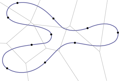
(a)

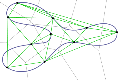
(b)

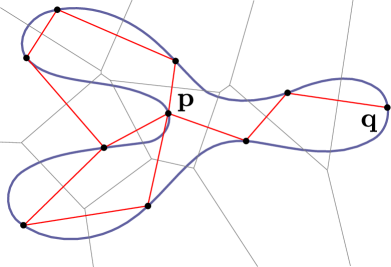
(c)

(d)

Figure 2: (a) the Voronoi complex of a point sample from a closed curve and (b) the dual Delaunay graph; (c) the Delaunay graph restricted to the curve. In order to make the graph homeomorphic to the curve, the sample density has to be increased (d).

The Voronoi cell of a point $\mathbf{p}$ in a set of points $L$ is:

$$V_{\mathbf{p}}=\{\mathbf{x}\in\mathbb{R}^{d}\>|\;\|\mathbf{x}-\mathbf{p}\|\leq\|\mathbf{x}-\mathbf{q}\|,\forall\mathbf{q}\in L,\mathbf{q}\neq\mathbf{p}\}$$

The intersection of two Voronoi cells in $\mathbb{R}^{d}$ may be either empty or a linear face of dimension $d-1$. Likewise, the intersection of $n$ such cells is either empty or a linear face of dimension $d-n+1$, with a minimum of 0. For example, the intersection of $d$ cells is either empty or an edge (i.e. dimension 1) and the intersection of $d+1$ cells is either empty or a single point (i.e. dimension 0). The Voronoi cell together with the faces of all dimensions form the Voronoi complex of $L$. Fig. 2(a) shows an example of a Voronoi complex for a set of points in $\mathbb{R}^{2}$.

A finite set of point $L$ in $\mathbb{R}^{d}$ is said to be non degenerate if no $d+2$ Voronoi cells have a non-empty intersection.

The Delaunay graph of a finite set of points $L$ is dual to the Voronoi complex, in the sense that two points $\mathbf{p}$ and $\mathbf{q}$ in $L$ are connected in the Delaunay graph if the intersection of the two corresponding Voronoi cells is not empty. The Delaunay simplicial complex $\mathcal{D}(L)$ is defined by extending the above idea to simplices of higher dimensions: a face $\sigma$ of dimension $n$ is in $\mathcal{D}(L)$ iff the intersection of the Voronoi cells corresponding to the $n+1$ points in $\sigma$ is non-empty. If the set $L$ is non-degenerate, $\mathcal{D}(L)$ will contain simplices of dimension at most $d$. Fig. 2(b) shows the Delaunay graph corresponding to the Voronoi complex in Fig. 2(a).

III-A Restricted Delaunay complex

The concept of restricted Delaunay graph was already defined in [3], albeit with a slightly different terminology.

Let $M\subseteq\mathbb{R}^{d}$ be a manifold of dimension $k$. The restricted Voronoi cell of $\mathbf{p}$ w.r.t a manifold $M$ is:

$$V_{\mathbf{p},\,M}=V_{\mathbf{p}}\cap M$$

The restricted Delaunay graph of $L$ with respect to $M$ is a graph where points $\mathbf{p}$ and $\mathbf{q}$ are connected iff $V_{\mathbf{p},\,M}\,\cap\,V_{\mathbf{q},\,M}\neq\emptyset$. Fig. 2(c) shows the restricted Delaunay graph with respect to a closed curve. Note that the restricted Delaunay graph is a subset of the Delaunay graph (Fig. 2(a)) for the same set of points.

The restricted Delaunay simplicial complex $\mathcal{D}_{M}(L)$ is the simplicial complex obtained from the complex of the restricted Voronoi cells $\mathcal{V}_{M}(L)$.

III-B Homeomorphism and $\varepsilon$-sample

Note that the restricted Delaunay graph in Fig. 2(c) is not homeomorphic to the closed curve $M$. For instance, point $\mathbf{p}$ has only one neighbor, instead of two, whereas $\mathbf{q}$ has four. This means that the piecewise-linear curve $\mathcal{D}_{M}(L)$ has one boundary point and (at least) one self-intersection and therefore it does not represent $M$ correctly.

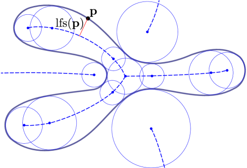
Figure 3: The medial axis (dashed line) of a closed curve and the local feature size at a point $\mathbf{p}$.

The medial axis of $M$ is the closure of the set of points that are the centers of maximal balls, called medial balls, whose interiors are empty of any points from $M$. The local feature size at a point $\mathbf{p}\in M$ is the distance of $\mathbf{p}$ from the medial axis. The global feature size of a compact manifold $M$ is the infimum of $\mathrm{lfs}(\mathbf{x})$ over all $M$. Fig. 3 describes the medial axis (dashed blue line) for the manifold in Fig. 2. The local feature size of point $\mathbf{p}$ in figure is equal to the length of the red segment.

By definition, the set $L$ is an $\varepsilon$-sample of $M$ if for all points $\mathbf{x}\in M$ there is at least one point $\mathbf{p}\in L$ such that $\|\mathbf{x}-\mathbf{p}\|\leq\varepsilon\cdot\mathrm{lfs}(\mathbf{x})$.

Theorem III.1

Under the additional condition that $M$ is smooth, there exists an $\varepsilon>0$ such that if the set $L$ is an $\varepsilon$-sample of $M$, then $\mathcal{D}_{M}(L)\approx M$ [12].

Slightly different values of $\varepsilon$ ensuring the validity of theorem III.1 are reported in the literature. It will suffice to our purposes that such positive values exist. The effect of the above theorem is exemplified in Fig. 2(d): as the density of $L$ increases the restricted Delaunay graph becomes homeomorphic to the curve.

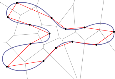
(a)

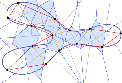
(b)

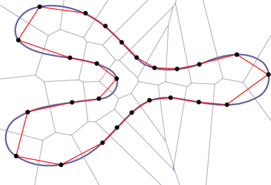
(c)

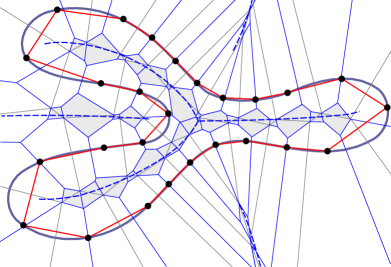
(d)

Figure 4: (a) the restricted Delaunay complex is homeomorphic to the curve; (b) the witness complex, however, includes further edges, due to the extent of second order Voronoi regions; (c) after increasing the sample density, the restricted Delaunay complex remains homeomorphic to the curve and (d) coincides with the witness complex.

III-C Witness complex

The notion of a witness complex is tightly related to the competitive Hebbian rule described in [3] and, at least historically, descends from the latter.

Given a set of point $L\in\mathbb{R}^{d}$, a weak witness of a simplex $\sigma\subset L$ is a point $\mathbf{x}\in\mathbb{R}^{d}$ for which $\|\mathbf{x}-\mathbf{a}\|\leq\|\mathbf{x}-\mathbf{b}\|$ for all $\mathbf{a}\in\sigma$ and $\mathbf{b}\in L-\sigma$. A strong witness is a weak witness $\mathbf{x}$ for which $\|\mathbf{x}-\mathbf{a}_{i}\|=\|\mathbf{x}-\mathbf{a}_{j}\|$ for all $\mathbf{a}_{i},\mathbf{a}_{j}\in\sigma$. Note in passing that all points belonging to the intersection of two Voronoi cells $V_{\mathbf{a}}$ and $V_{\mathbf{b}}$ are strong witnesses for the edge $(\mathbf{a},\mathbf{b})$. The set of all weak witnesses for this same edge is also called the second order Voronoi cell of the two points $\mathbf{a}$ and $\mathbf{b}$ [5].

The witness complex $\mathcal{C}^{W}(L)$ is the simplicial complex that can be constructed from the set of points $L$ with a specific set of witnesses $W$.

Theorem III.2

Let $L\subset\mathbb{R}^{d}$ be a set of points. If every face of a simplex $\sigma\subseteq L$ has a weak witness in $\mathbb{R}^{d}$, then $\sigma$ has a strong witness $\mathbb{R}^{d}$ [13] .

As a corollary, this theorem implies that $\mathcal{C}^{W}(L)\subseteq\mathcal{D}(L)$ and in the limit the two complexes coincide, when $W\equiv\mathbb{R}^{d}$.

Theorem III.2 does not extend to restricted Delaunay complexes, namely when the witnesses belong to a manifold $M$. A counterexample is shown in Fig. 4(a), which describes the witness complex constructed from the same $L$ in Fig. 2(d) using the whole $M$ as the set of witnesses. The second-order Voronoi regions (in blue) for the connections (in orange) which do not belong to the restricted Delaunay graph, do intersect the closed curve. This means that $M$ contains weak witnesses for connections for which $M$ itself contains no strong witnesses, as the definition of $\mathcal{D}_{M}(L)$ would require.

Theorem III.3

If $M$ is a compact smooth manifold without boundary of dimension 1 or 2, there exists an $\varepsilon>0$ such that if $L$ is an $\varepsilon$-sample of $M$, the following implication holds: if every face of a simplex $\sigma\subseteq W$ has a weak witness, then $\sigma$ has a strong witness [14].

Like before, this implies that $\mathcal{C}^{W}_{M}(L)$, i.e. the witness complex restricted to $M$, is included in $\mathcal{D}_{M}(L)$ and the two coincide in the limit, when $W\equiv M$. As a corollary, Theorem III.3 also implies that $\mathcal{D}_{M}(L)\approx M$. Specific, viable values for $\varepsilon$ are reported in [14], but once again it will suffice to our purposes that such positive values exist.

The effect of theorem III.3 is described in Fig. 4(c) and (d): by further increasing the density of $L$, the witness complex $\mathcal{C}^{W}_{M}(L)$ coincides with $\mathcal{D}_{M}(L)$, when $W$ is the entire curve. Fig. 4(c) shows that, as the density of $L$ increases, the second-order Voronoi regions for the violating connections ‘move away’ from $M$ and tend to aggregate around the medial axis.

The other side of the medal is represented by:

Theorem III.4

For manifolds of dimension greater than 2, no positive value of $\varepsilon$ can guarantee that every face of a simplex $\sigma\in\mathcal{C}_{M}^{W}(L)$ having a weak witness also has a strong witness [15].

III-D Finite samples and noise

As fundamental as it is, Theorem III.3 is not per se sufficient for our purposes. First, it assumes the potential coincidence of $W$ with $M$, which would require an infinite sample, and, second, its proof requires that $L\subset M$, which is not necessarily true with vector quantization algorithms and/or in the presence of noise.

An $\varepsilon$-sparse sample $L$ is such that the pairwise distance between any two points of $L$ is greater than $\varepsilon$. A $\delta$-noisy sample $L$ is such that no points in $L$ are farther than $\delta$ from $M$.

Theorem III.5

If $M$ is a compact smooth manifold without boundary of dimension 1 or 2, there exist positive values of $\varepsilon$ and $\delta$ such that if $W$ is a $\delta$-noisy $\delta$-sample of $M$ and $L$ is a $\delta$-noisy, $\varepsilon$-sparse $(\varepsilon+\delta)$-sample of $M$ then $\mathcal{C}_{M}^{W}(L)\subseteq\mathcal{D}_{M}(L)$ [16].

Actually, a stronger result holds in the case of curves, stating that $\mathcal{C}_{M}^{W}(L)$ and $\mathcal{D}_{M}(L)$ will coincide. For surfaces this guarantee cannot be enforced due to a problem that is described in Fig. 5. Even if $L$ is non-degenerate, in fact, it may contain points that are arbitrarily close to a co-circular configuration, thus making the area of the second-order Voronoi region in the midst so small that no density condition on $W$ could ensure the presence of an actual witness. This means that, in a general and non-degenerate case, a few connections will be missing from $\mathcal{C}^{W}(L)$.

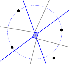
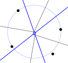
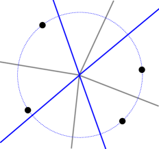
Figure 5: As the points approach co-circularity, the second order Voronoi region in the midst becomes arbitrarily small.

IV Self-Organizing Adaptive Map (SOAM)

The intuitive idea behind the SOAM algorithm introduced here, which is derived from the GWR algorithm [9], is pretty simple. Points like $\mathbf{p}$ and $\mathbf{q}$ in Fig.2(c), whose neighborhoods are not of the expected kind, are true symptoms of the fact that network structure, i.e. the witness complex $\mathcal{C}_{M}^{W}(L)$, is not homeomorphic to the input manifold $M$. Symptoms like these are easily detectable, provided that the expected dimension of $M$ is known. Then, in the light of the above theoretical results, the network might react by just increasing the density of its units. Given that the target density is function of the local feature size of $M$, new units need only be added where and when required.

Figure 6: The star, closure and link of a vertex in a simplicial complex of dimensions 1 (above) and 2 (below).

IV-A Topology-driven state transitions

The state of units in a SOAM is determined according to the topology of their neighborhoods. Given a unit $u_{i}$, its neighborhood in a simplicial complex is defined as the star $\mathrm{St}(u_{i})$, consisting of $u_{i}$ together with the edges and triangles that share $u_{i}$ as a vertex. The closure of a star $\mathrm{Cl}(\mathrm{St}(u_{i}))$ is obtained by adding all simplices in $\mathcal{C}(L)$ having a non-null intersection with $\mathrm{St}(u_{i})$. Finally, the link is then defined as

$$\mathrm{Lk}(u_{i})=\mathrm{Cl}(\mathrm{St}(u_{i}))-\mathrm{St}(u_{i})$$

The eight possible states for units in a SOAM are:

• The default state of any newly-created unit.

• The value of the firing counter $f$ (see below) of the unit is greater than a predefined threshold $T_{f}$.

• The unit is habituated and all the units in its link are habituated as well.

• The link of unit is homeomorphic to an half-sphere.

• The link of unit is homeomorphic to a sphere.

• The unit is an half-disk and all its neighbors are regular (see below).

• The unit is a disk and all its neighbors are regular.

• The unit is over-connected, i.e. its link exceeds a topological sphere. More precisely, the link contains a sphere plus some other units and, possibly, connections.

In the case of dimension 2, a unit whose link is a disk but contains three units only is a tetrahedron and, by definition, is considered singular as well.

Note that all the above topological conditions can be determined combinatorially and hence very quickly. On the other hand, the actual test to be performed depends on the expected dimension of the input manifold $M$. In Fig. 6 on the right, the two links above and below are disks in dimension 1 and 2, respectively. For instance, in a complex of dimension 2, a link like the one above on the right in Fig. 6 would not be a disk at all.

Two further, derived definitions will be convenient while describing the SOAM algorithm:

• The unit is in one of these states: half-disk, disk, boundary or patch.

• In this version of the algorithm, only the patch state is deemed stable.

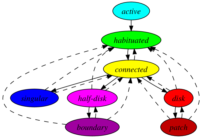
Figure 7: Topology-driven state transitions for units in a SOAM. The same state colors are used in other figures.

IV-B Adaptive insertion thresholds

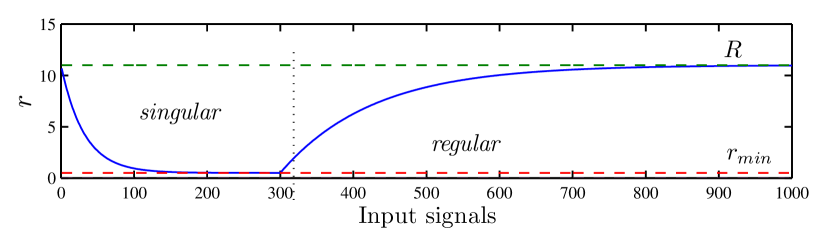
Figure 8: The overall model of habituation and dishabituation of insertion thresholds, with different time constants $\tau$.

The model adopted in the GWR algorithm for the exponential decay of the firing counter $f$ has been derived from the biophysics of the habituation of neural synapses [9]. The equation that rules the model is:

$$h(t)=H-\frac{1}{\alpha}(1-\mbox{e}^{-\alpha\cdot t/\tau})$$ (1)

where $h(t)$ is the value being adapted, as a function of time $t$, $H$ is the maximum, initial value and $\alpha$ and $\tau$ are suitable parameters. Equation (1) is the solution of the differential equation:

$$\frac{\mbox{d}h(t)}{\mbox{d}t}=\frac{\alpha\cdot(H-h(t))-1}{\tau}$$ (2)

The reverse model, of dishabituation, is also considered here:

$$h(t)=H-\frac{1}{\alpha}\cdot\mbox{e}^{(-\alpha\cdot t)/\tau)}$$ (3)

which in turn is the solution of:

$$\frac{\mbox{d}h(t)}{\mbox{d}t}=\frac{\alpha}{\tau}\cdot(H-h(t))$$ (4)

In the SOAM algorithm, the overall model of habituation and dishabituation is adopted for adapting the local insertion thresholds $r$ of units (see below). More precisely, the value of $r$ for singular units decays exponentially to a value $r_{min}$, while the state persists, whereas the value of $r$ of regular units grows asymptotically to the initial value $R$.

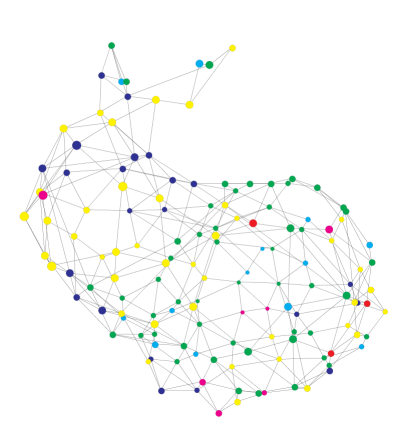
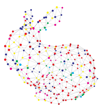
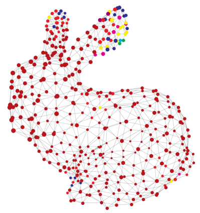
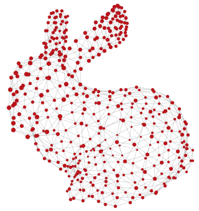
Figure 9: A SOAM reconstructing the the Stanford bunny. In the final structure, all 435 units are in the stable state.

IV-C The SOAM algorithm

Initially, the set $L$ of units contains two units $u_{0}$ and $u_{1}$ only, with positions assigned at random according to $P(\mathbf{\xi})$. The $C$ of connections is empty. All firing counters $f$ and insertion thresholds $r$ of newly created units are initialized to $F$ and $R$, respectively.

1. Receive the next sample $\mathbf{\xi}$ from the input stream.

2. Determine the indexes $b$ and $s$ of the two units that are closest and second-closest to $\mathbf{\xi}$, respectively

   $$\mathbf{p}_{b} = \arg\min_{u_{i}\in A}\|\mathbf{\xi}-\mathbf{p}_{i}\|$$

   $$\mathbf{p}_{s} = \arg\min_{u_{i}\in A-{u_{b}}}\|\mathbf{\xi}-\mathbf{p}_{i}\|$$

3. Add connection $(b,s)$ to $C$, if not already present, otherwise set its $age$ to $0$.

4. Unless $u_{b}$ is stable, increase by one the $age$ of all its connections. Remove all connections of $u_{b}$ whose $age$ exceeds a given threshold $T_{age}$. Then, remove all units that remain isolated.

5. If $u_{b}$ is at least habituated and $\|\mathbf{\xi}-\mathbf{p}_{b}\|>r_{b}$, create a new unit $u_{n}$:

   • Add the new unit $u_{n}$ to $L$

   • Set the new position: $\mathbf{p}_{n}=(\mathbf{p}_{b}+\mathbf{\xi})/2$

   • Add new connections $(b,n)$ $(n,b)$ to $C$

   • Remove the connection $(b,s)$ from $C$

   Else, if $u_{b}$ is at least habituated and $\|\mathbf{p}_{s}-\mathbf{p}_{b}\|<r_{min}$, merge $u_{b}$ and $u_{s}$:

   • Set the new position: $\mathbf{p}_{b}=(\mathbf{p}_{b}+\mathbf{p}_{s})/2$

   • For all connections $(s,x)$, add a new connection $(b,x)$ to $C$, if not already present

   • Remove all connections $(s,x)$ from $C$

   • Remove $u_{s}$ from $L$

6. Adapt the firing counters of $u_{b}$ and of all units $u_{nb}$ that are connected to $u_{b}$

   $$\Delta f_{b} = (\alpha_{h}\cdot(F-f_{b})-1)/\tau_{f}$$

   $$\Delta f_{nb} = (\alpha_{h}\cdot(F-f_{nb})-1)/\tau_{f,\,n}$$

7. Update the state of $u_{b}$, according to the value of $f_{b}$ and the topology of its neighborhood of connected units.

8. If the unit $b$ is singular, adapt its insertion threshold

   $$\Delta r_{b}=(\alpha_{r}\cdot(R-r_{b})-1)/\tau_{r,\,hab}$$

   Else, if the unit $b$ is regular, adapt its insertion threshold in the opposite direction

   $$\Delta r_{b}=((\alpha_{r}/\tau_{r,\,dis})\cdot(R-r_{b})$$

9. Unless $u_{b}$ is stable, adapt its positions and those of all connected units $u_{nb}$

   $$\Delta\mathbf{p}_{b} = \eta_{b}\cdot f_{b}\cdot(\mathbf{\xi}-\mathbf{p}_{b})$$

   $$\Delta\mathbf{p}_{nb} = \eta_{nb}\cdot f_{nb}\cdot(\mathbf{\xi}-\mathbf{p}_{nb})$$

   Else, if $u_{b}$ is stable, adapt only the position of $u_{b}$ itself

   $$\Delta\mathbf{p}_{b}=\eta_{stable}\cdot f_{b}\cdot(\mathbf{\xi}-\mathbf{p}_{b})$$

   where, typically, $\eta_{stable}\ll\eta_{b}$.

10. If further inputs are available, return to step (1), unless some termination criterion has been met.

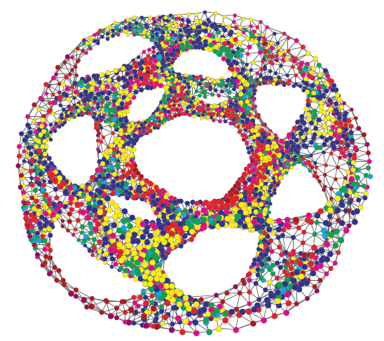
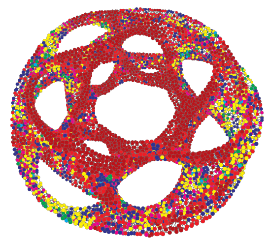
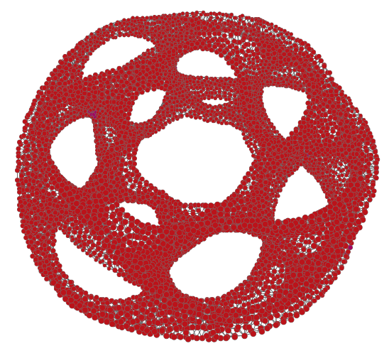
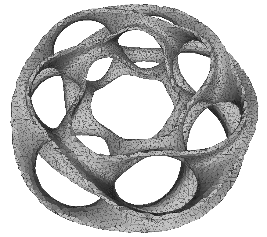
Figure 10: A SOAM reconstructing the heptoroid, which has genus 22. The final structure includes 10,103 units and has been obtained after some 8M input signals.

V Experimental evidence

Practical experiments have been performed to assess the properties of the SOAM algorithm, in particular with surfaces, as this is by far the trickiest case. The test set adopted includes 32 triangulated meshes, downloaded from the AIM@SHAPE repository [17]. The reason for this choice is that the homeomorphism with a triangulated mesh can be easily verified. In fact, two closed, triangulated surfaces are homeomorphic if they are both orientable (or non-orientable) and have the same Euler characteristic [11]:

$$\chi=vertex-edges+faces$$

Meshes in the test set have genus (i.e. the number of tori whose connected sum is homeomorphic to the given surface [11]), ranging from 0 to 65. All meshes were rescaled to make each bounding box have a major size of 256. In the experiments, mesh vertices were selected at random, with uniform distribution.

For completeness, a few test have also been performed with meshes with simple boundaries and with non-orientable surfaces (e.g. the Klein bottle), directly sampled from parametric expressions.

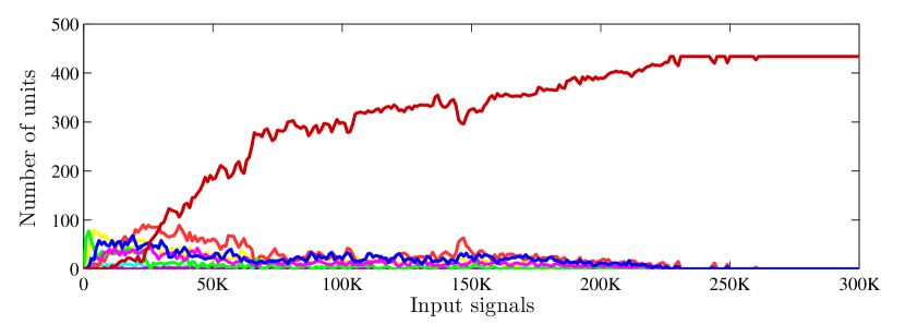
Figure 11: Typical run of the SOAM algorithm for the Stanford bunny reconstruction. Each line charts the number of units in the corresponding state/color.

V-A Topological convergence

For the whole set of triangulated meshes and in the absence of noise, it has been possible to make the SOAM reach a condition where all units were stable and the resulting structure was homeomorphic to the input mesh. Better yet, it has been possible to identify a common set of algorithm parameters (apart from the dimension of $M$) that, under conditions to be clarified below, proved to be adequate to the whole test set.

The typical, observed run of the adaptation process is charted in Fig. 11, which refers to the input mesh of 72,027 vertices for the process in Fig. 9. As we can see, the number of stable units (dark red line) in the SOAM grows progressively until a level of equilibrium is reached and maintained from that point on. In contrast, singular nodes (blue line) tend to disappear, although occasional onsets may continue for a while, for reasons that will be explained in short. Needless to say, in the most complex test cases a similar level of equilibrium was reached only after a much larger number of signals, but substantially the same behaviour has been observed in all successful runs.

V-B Algorithm parameters and their effect

All values for algorithm parameters reported here belong to the common set that has been identified empirically.

The values $\eta_{b}=0.05$ and $\eta_{nb}=0.0005$ for unit positions are slightly higher than those suggested in the literature, as it emerged that an increased mobility of units in pre-stable states accelerates the process. Actually, this accentuated mobility also proved to be the way the problem described in Fig. 5 could be solved. In fact, only with much lower values of $\eta_{b}$ and $\eta_{nb}$ the occasional small ‘holes’ in a diamond of four units became persistent and could not be closed. A possible explanation, to be fully investigated yet, is that the higher mobility of units acts like a ‘simulation of simplicity’ [18], that is, a perturbation that makes low-probability configurations ineffective.

The values $\tau_{f}=3.33$ and $\tau_{f,\,n}=14.33$ for firing counters, with threshold $T_{f}=0.243$ were chosen initially and never changed afterwards.

In contrast, the values $\tau_{r,\,hab}=3$ for insertion thresholds require some care, as a shorter time constant may produce an excessive density of units and a longer one may slow down the process significantly. In addition, the appropriate combination with the values $\tau_{r,\,dis}=9$, $T_{age}=30$ $\eta_{stable}=0.02$ solves a problem with the connection aging mechanism. The aging mechanism, in fact, is meant to cope with the mobility of units during the adaptation process: any connection becoming unsupported by witnesses will age rapidly and eventually be removed. The drawback is that it acts in probability: in general, the probability of removing a connection is inversely proportional to the probability of sampling a supporting witness, which is not the same as having no witness at all. In all borderline cases, which are particularly frequent when - once again - four points approach co-circularity, connections are removed and created in a sort of ‘blinking’ behavior.

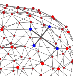
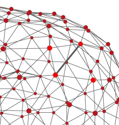
Figure 12: Edge flipping in a SOAM.

In step 4 of the algorithm, the aging mechanism is simply stopped for connections between stable units. From that point on, any ‘counter-witness’ to the correctness of the triangulation will create an extra connection that turns a set of four points into a singular tetrahedron, also resuming the aging mechanism. The violating connection will be removed eventually and the stable state will be established again. Overall, the resulting effect, depicted in Fig. 12, is very similar to edge flipping [10]. With an appropriate choice of the above values, occasional edge-flippings will not increase the density of units. Episodes of this kind may continue to occur after the network has first reached stability.

As one may expect, the maximum and minium insertion thresholds, $R$ and $r_{min}$ are critical parameters, since they rule the properties of the the SOAM as an $\varepsilon$-sample of the input manifold. Surprisingly however, setting those values proved less critical in practice. With a proper setting of $\tau_{r,\,hab}$, the density of units in the SOAM increases only when and as required, so that $r_{min}$ just acts as a lower threshold which is seldom reached, as proved by the fact that the merge in step 5 in the algorithm occurred very rarely. This could also be due to the entropic attitude of the algorithm, which promotes unit sparseness. The adopted value $r_{min}=0.5$ is equal to twice the maximum distance between neighboring points in the input data sets.

The parameter $R$ defines the minimum network density and hence the desired quality of the reconstruction. On the other hand, for reasons not yet completely clear from a theoretical standpoint, $R$ played no role in determining convergence. For instance, the value $R=25$, i.e. 10% of the major size of any bounding box, proved adequate in all cases. A possible explanation is that the high mobility of units makes it highly improbable the occurrence of false positives, intended as stable network configurations that do not represent $M$. Perhaps due to similar reasons, adapting the insertion threshold also of boundary units proved unnecessary, at least with closed surfaces, to ensure convergence.

             

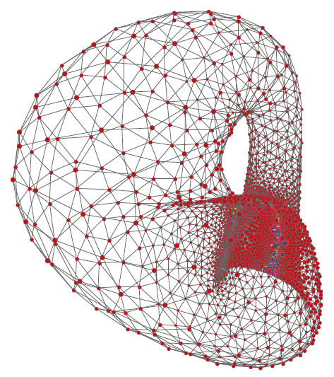
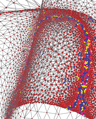
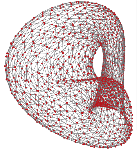
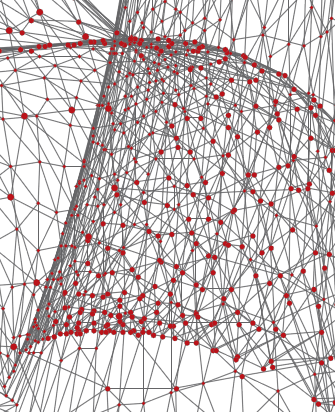
Figure 13: The Klein bottle is not a manifold in $\mathbb{R}^{3}$ (above): singular units in the SOAM mark the self-intersections. The same surface is a manifold in $\mathbb{R}^{4}$ and could be correctly reconstructed (below).

V-C When adaptation fails

Two kinds of symptoms may signal the failure of the network adaptation process:

1. Persistence of non-regular units, typically connected ones

2. Persistence of singular units

The causes of a) could be twofold. Either the input dataset is not a $\delta$-sample of the manifold $M$, in the sense of Theorem III.5, or, in the light of the same theorem, the value of $r_{min}$ is too low, in the sense that the network eventually became an $\varepsilon$-sample too fine for the $\delta$-sample represented by the input dataset.

Symptom b), on the other hand, could be due either to a too high value for $r_{min}$, which can be fixed easily, or to noise. In agreement with Theorem III.5, experiments show that the effects of noise on convergence are ‘on-off’: up to a certain value of the noise threshold, the process, albeit slowed down, continues to converge; beyond that value, symptom b) always occurs and the adaptation is doomed to fail. Given that the actual noise threshold depends on the global feature size of $M$, its value may be difficult to compute beforehand. As a compensation, SOAM failures are typically very localized, thus showing which parts of $M$ are more problematic.

VI Conclusions and future work

The design of the SOAM algorithm relies heavily on the theoretical corpus presented in the previous sections. Experiments show that these results may be very effective in enforcing stronger topological guarantees for growing neural networks. Clearly, many aspects still remain to be clarified. For one, the guarantee that a SOAM will eventually reach a stable configuration - in the sense described above - for any non-defective input dataset remains to be proved.

Nevertheless, at least in the author’s opinion, a strong point of the SOAM algorithm is that it produces clear signs of a convergence - or lack thereof - whose correctness, in the line of principle, is verifiable. In addition, experiments seem to suggest that, in some sense, the algorithm exceeds known theoretical results and it may lead to new solutions for known problems [16].

About future developments, the current limitations about the dimension of the manifold might be overcome along the lines suggested in [19], although this would require switching to the weighted version of the Delaunay complex. Nonetheless, again in the author’s opinion, a great potential of the SOAM algorithm presented relates to tracking non-stationary input manifolds, which is the reason why, in designing the algorithm itself, care has been taken to keep all transitions reversible.

References

- [1] T. Kohonen, Self-organizing maps. Springer-Verlag, 1997.
- [2] T. Martinetz and K. Schulten, “A ”neural gas” network learns topologies,” in Artificial Neural Networks, T. Kohonen, K. Mäkisara, O. Simula, and J. Kangas, Eds. Elsevier, 1991, pp. 397–402.
- [3] ——, “Topology representing networks,” Neural Networks, vol. 7, no. 3, pp. 507–522, 1994.
- [4] F. Cazals and J. Giesen, “Delaunay triangulation based surface reconstruction,” in Effective Computational Geometry for Curves and Surfaces, J.-D. Boissonnat and M. Teillaud, Eds. Springer-Verlag, 2006.
- [5] T. Martinetz, S. Berkovich, and K. Schulten, “Neural-gas network for vector quantization and its application to time-series prediction,” IEEE Trans. Neural Networks, vol. 4, no. 4, pp. 558–569, Jul 1993.
- [6] E. Erwin, K. Obermayer, and K. Schulten, “Self-organizing maps: ordering, convergence properties and energy functions,” Biological Cybernetics, vol. 67, pp. 47–55, 1992.
- [7] B. Fritzke, “A growing neural gas network learns topologies,” in Advances in Neural Information Processing Systems 7. MIT Press, 1995, pp. 625–632.
- [8] J. Bruske and G. Sommer, “Dynamic cell structure learns perfectly topology preserving map,” Neural Comput., vol. 7, no. 4, pp. 845–865, 1995.
- [9] S. Marsland, J. Shapiro, and U. Nehmzow, “A self-organising network that grows when required,” Neural Networks, vol. 15, no. 8-9, pp. 1041–1058, 2002.
- [10] H. Edelsbrunner, Geometry and Topology for Mesh Generation. Cambridge University Press, 2006.
- [11] A. Zomorodian, Topology for Computing. Cambridge University Press, 2005.
- [12] N. Amenta and M. Bern, “Surface reconstruction by voronoi filtering,” in SCG ’98: Proc. of the 14th annual symp. on Computational geometry. ACM, 1998, pp. 39–48.
- [13] V. de Silva and G. Carlsson, “Topological estimation using witness complexes,” in Proc. of Eurographics Symp. on Point-Based Graphics, 2004, pp. 157–166.
- [14] D. Attali, H. Edelsbrunner, and Y. Mileyko, “Weak witnesses for delaunay triangulations of submanifolds,” in SPM ’07: Proc. 2007 ACM symp. on Solid and physical modeling. ACM, 2007, pp. 143–150.
- [15] S. Oudot, “On the topology of the restricted delaunay triangulation and witness complex in higher dimensions,” CoRR, vol. abs/0803.1296, 2008.
- [16] L. J. Guibas and S. Y. Oudot, “Reconstruction using witness complexes,” in SODA ’07: Proc. of the 18th annual ACM-SIAM symp. on Discrete algorithms, 2007, pp. 1076–1085.
- [17] B. Falcidieno, “Aim@shape project presentation,” Shape Modeling and Applications, International Conference on, p. 329, 2004.
- [18] H. Edelsbrunner and E. P. Mücke, “Simulation of simplicity: a technique to cope with degenerate cases in geometric algorithms,” in SCG ’88: Proc. of the 4th annual symp. on Computational geometry. ACM, 1988, pp. 118–133.
- [19] J.-D. Boissonnat, L. J. Guibas, and S. Y. Oudot, “Manifold reconstruction in arbitrary dimensions using witness complexes,” in SCG ’07: Proc. of the 23rd symp. on Computational geometry. ACM, 2007, pp. 194–203.