Markovian Monte Carlo program EvolFMC v.2 for solving QCD evolution equations

Abstract

We present the program EvolFMC v.2 that solves the evolution equations in QCD for the parton momentum distributions by means of the Monte Carlo technique based on the Markovian process. The program solves the DGLAP-type evolution as well as modified-DGLAP ones. In both cases the evolution can be performed in the LO or NLO approximation. The quarks are treated as massless. The overall technical precision of the code has been established at $5\times 10^{-4}$. This way, for the first time ever, we demonstrate that with the Monte Carlo method one can solve the evolution equations with precision comparable to the other numerical methods.

PACS: 12.38.-t, 12.38.Bx, 12.38.Cy

IFJPAN-IV-2008-7

PROGRAM SUMMARY/NEW VERSION PROGRAM SUMMARY

Manuscript Title: The Markovian Monte Carlo program EvolFMC v.2 for solving QCD evolution equations
Authors: S. Jadach, W. Płaczek, M. Skrzypek, P. Stokłosa
Program Title: EvolFMC v.2
Journal Reference:
Catalogue identifier:
Licensing provisions: none
Programming language: C++
Computer: PC, Mac
Operating system: Linux, Mac OS X
RAM: less than 256 MB
Number of processors used: 1
Supplementary material:
Keywords: Monte Carlo, evolution equations, Markovian process, radiative corrections, QCD, NLO, LHC, HERA, DGLAP, PDF
PACS: 12.38.-t, 12.38.Bx, 12.38.Cy
Classification:
External routines/libraries: ROOT
Subprograms used:
Nature of problem:
Solution of the QCD evolution equations for the parton momentum distributions of the DGLAP- and modified-DGLAP-type in the LO and NLO approximations.
Solution method:
Monte Carlo simulation of the Markovian process of a multiple emission of partons.
Restrictions:
(1) Limited to the case of massless partons.
(2) Implemented in the LO and NLO approximations only.
(3) Weighted events only.
Unusual features:
Modified-DGLAP evolutions included up to the NLO level.
Additional comments:
Technical precision established at $5\times 10^{-4}$.
The EvolFMC version 1 was described in [1], but the actual code was not published.
Running time:
For the $10^{6}$ events at 100 GeV: DGLAP NLO: 27s; C’-type modified DGLAP NLO: 150s (MacBook Pro with Mac OS X v.10.5.5, 2.4 GHz Intel Core 2 Duo, gcc 4.2.4, single thread);

LONG WRITE-UP

1 Introduction

The evolution equations (EVEQs) for parton distribution functions (PDFs) and parton momentum distributions are one of the most efficient tools in calculating the radiative corrections in Quantum Chromodynamics (QCD) because they perform resummation of certain types of corrections up to infinite order. The PDFs are indispensable in any analysis of scattering processes which involve hadrons. The non-perturbative information on hadron structure, for the time being not calculable, is extracted from the experimental data and then used to create the PDFs at low energy scale. Among various types of evolution equations the most important is the family of the DGLAP-type equations [2]. Other widely used types of the EVEQs include BFKL [3], CCFM [4] or IREE [5]. In this paper we will discuss the DGLAP and modified-DGLAP types of EVEQs. However, a comment on the relation to CCFM EVEQs will be made.

There are various numerical methods of solving the DGLAP-type EVEQs: Mellin transforms [6], evolution on a finite grid [7, 8, 9], expansion in Laguerre polynomials [10, 11], expansion in Chebyshev polynomials [12, 13], etc. The Monte Carlo (MC) methods differ from the other numerical techniques because, in addition to providing the inclusive parton distributions, they supply also the complete tree of parton emissions during evolution. This allows one to construct the MC Parton Shower programs which provide the actual four-momenta of emitted quarks and gluons – a necessary input for any realistic analysis which must include experimental apparatus effects. One can find numerous implementations of the leading order DGLAP evolution in the MC Parton Shower codes; let us quote just a few examples: PYTHIA [14, 15], HERWIG [16, 17], ARIADNE [18], GR$@$PPA [19, 20]. So far the MC methods have not been considered as a realistic alternative to the other numerical methods of solving EVEQs due to low precision and long time of computation. The presented here MC code EvolFMC is intended to fill-in this gap, profiting from the dramatic increase of the CPU power over two decades since NLO DGLAP evolution was formulated and solved numerically for the first time. It will be demonstrated in the following with the examples of numerical calculations that EvolFMC can solve the (modified) DGLAP-type EVEQs with high precision ($5\times 10^{-4}$ at least) within a reasonable CPU time.

The program EvolFMC solves the EVEQs for the parton momentum distributions by means of the MC simulation of the multiple emission of partons in the cascade. The emission process is of the Markovian type, i.e. each emission depends on the information from the previous emission only. The algorithms are constructed on the basis of the Markovian process with simplified emission kernels which retain only the leading singularities. The complete kernels in the leading and next-to-leading approximation are then recovered by the standard reweighting procedure.

The evolution is two-dimensional ($x$ and $t$) by construction. However, the azimuthal angle can always be added with a flat probability density distribution. Having identified the evolution time with certain kinematical variable, one can then reconstruct the four-momenta of all emitted partons. Such a procedure of reconstructing the four-momenta is, of course, exact only in the LO approximation. In the NLO approximation the differential distributions will be strictly speaking correct only in the ”inclusive” sense of the overall normalisation. This is, however, the common (and in fact the only available) approach to the Parton Shower MCs. It should be mentioned here that recently there have been a few attempts to construct a true NLO Parton Shower algorithm with the help of ”fully unintegrated” or ”exclusive” partonic functions [21, 22, 23, 24].

Apart from the standard DGLAP, two modified-DGLAP-type EVEQs can be solved by EvolFMC. The modifications involve a change of the argument of the coupling constant together with the introduction of a finite cut-off on its minimal value. The program works in the weighted mode only. The first version of the code, the EvolFMC v.1, was described in [1], but the actual code was not published. The version v.1 solved modified-DGLAP-type in the LO approximation only. The NLO evolution was available only in the standard DGLAP case. Also the structure of the code is rebuilt in version v.2.

Let us conclude this introduction with the following remark. The MC approach to EVEQs has one important general advantage: with the help of the reweighting technique it is easy to introduce into evolution some additional effects or modifications. As an example let us mention the possibility of emulating the CCFM-type evolution. From the algorithmic point of view, having generated the azimuthal angles and reconstructing the transverse momenta of the partons in the shower, one can trivially construct the so-called “non-Sudakov” form factor and include it as a correcting weight. Of course, one has to remember that from the theoretical point of view the definition of the non-Sudakov form factor in the NLO case is a highly nontrivial problem; even the complete LO analysis is difficult in the context of the CCFM equation [25]. Additional modifications in evolution kernels can be done as well.

The paper is organized as follows. In Section 2 we give a short theoretical overview of the evolution equations and their solutions by means of MC methods. Section 3 describes in some detail the architecture of the presented MC code, EvolFMC version 2. Section 4 contains instructions on how to install the code on Linux and Mac OS X platforms. In Section 5 we present two demonstration programs included in the distributed version of the code. Section 6 contains a detailed study of the technical precision of EvolFMC at the level of $5\times 10^{-4}$. A short summary in Section 7 concludes the paper.

2 Theoretical background

In this short theoretical overview we will only give a few formulae and definitions necessary to explain the notation, to define the problem and to present the solution. For detailed derivations and technical description of the algorithms we refer the reader to the extensive bibliography, which we will present here in more detail. The short and elementary description of the solution of the DGLAP-type EVEQs in terms of the Markovian process and its MC realization in the LO approximation has been presented in Ref. [26]. The extension to the NLO level and comprehensive description of MC algorithms that solve the Markovian evolutions of PDFs and parton momentum distributions has been given in Refs. [1, 27]. The algorithms presented in [1] have been implemented in the first version of the code, EvolFMC v.1. The extension to the modified-DGLAP-type evolutions and the detailed description of appropriate modified-DGLAP Markovian algorithms has been given in Refs. [28, 29] for the LO case (implemented in EvolFMC v.1) and in Ref. [30] for the NLO approximation. The implementation of algorithms from Ref. [30] as well as re-organization of the implementation of the DGLAP-type algorithms from Ref. [1] has been done in the second version of the code, EvolFMC v.2, presented in this paper. Finally, in Ref. [13] the general and universal formalism of constructing Markovian algorithms, common for all DGLAP-type and modified-DGLAP-type evolutions, has been presented on the basis of the operator language. It is this formulation [13] that we will use in the rest of this section to describe the principles of the Markovian MC evolution.

The evolution equation and its solution in the form of a master iterative formula for the Markovian MC algorithm can be expressed as follows:

$$\partial_{t}{\bf D}(t)={\bf K}(t)\;{\bf D}(t),\;\;\;\hbox{i.e. }\;\;\partial_{t}D_{f}(t,x)=\sum_{f^{\prime}}\int_{0}^{1}dw\;\mathcal{K}_{ff^{\prime}}(t,x,w)D_{f^{\prime}}(t,w),$$ (1)

and

$$\begin{split}\bar{\bf E}{\bf D}(t)=\int_{t_{0}}^{t}dt_{1}\bigg{(}\int_{t_{1}}^{t}dt_{2}\bigg{[}&\int_{t_{2}}^{t}dt_{3}\bigg{\{}\dots\\ \dots\int_{t_{N-1}}^{t}dt_{N}\bigg{\{}&\bar{\bf E}{\bf K}^{R}(t_{N}){\bf G}_{{\bf K}^{V}}(t_{N},t_{N-1})+\bar{\bf E}{\bf G}_{{\bf K}^{V}}(t,t_{N-1})\delta_{t_{N}=t}\bigg{\}}\times\\ ~{}~{}~{}~{}~{}~{}~{}~{}~{}~{}~{}~{}~{}\vdots\\ \times&{\bf K}^{R}(t_{2}){\bf G}_{{\bf K}^{V}}(t_{2},t_{1})+\bar{\bf E}{\bf G}_{{\bf K}^{V}}(t,t_{1})\delta_{t_{2}=t}\bigg{]}\times\\ \times&{\bf K}^{R}(t_{1}){\bf G}_{{\bf K}^{V}}(t_{1},t_{0})+\bar{\bf E}{\bf G}_{{\bf K}^{V}}(t,t_{0})\delta_{t_{1}=t}\bigg{)}{\bf D}(t_{0}).\end{split}$$ (2)

Let us describe all the ingredients of eqs. (1) and (2).

• The multiplication of the matrices is understood as: $\sum_{f^{\prime}}\int_{0}^{1}dw$.

• $D_{f}(t,w)$ is the parton density function of the parton $f$.

• $\mathcal{K}_{ff^{\prime}}(t,x,w)$ is the generalized evolution kernel built from the real and virtual parts:

  $$\begin{split}\mathcal{K}_{ff^{\prime}}(t,x,w)=&\mathcal{K}^{V}_{ff^{\prime}}(t,x,w)+\mathcal{K}^{R}_{ff^{\prime}}(t,x,w),\\ \mathcal{K}^{V}_{ff^{\prime}}(t,x,w)=&-\delta_{ff^{\prime}}\delta_{x=w}\mathcal{K}^{v}_{ff}(t,x).\end{split}$$ (3)

• The operator $\bar{\bf E}$ is defined as $\{\bar{\bf E}\}_{f}(x)\equiv x$, i.e. it turns parton distributions into parton momentum distributions, whereas summing and integrating over final degrees of freedom means in the MC language that we generate all possible final state configurations without any constraints.

• ${\bf G}_{{\bf K}^{V}}$ is the solution of the evolution equation with the virtual kernel $\mathcal{K}^{V}_{ff^{\prime}}(t,x,w)$ only

  $$\{{\bf G}_{{\bf K}^{V}}(t,t^{\prime})\}_{ff^{\prime}}(x,w)=\delta_{ff^{\prime}}\delta_{x=w}\;e^{-\Phi_{f}(t,t^{\prime}|w)}.$$ (4)

• $\Phi_{f}(t,t^{\prime}|x)$ is the Sudakov form factor, expressed in terms of the real emission part of the evolution kernel

  $$\Phi_{f}(t,t^{\prime}|x)= \int\limits_{t^{\prime}}^{t}dt^{\prime\prime}\;\mathcal{K}^{v}_{ff}(t^{\prime\prime},x)=\sum_{f^{\prime}}\int\limits^{t}_{t^{\prime}}dt^{\prime\prime}\int\limits_{0}^{x}\frac{dx^{\prime}}{x}x^{\prime}\;\mathcal{K}^{R}_{f^{\prime}f}(t^{\prime\prime},x^{\prime},x)$$

  $$= \sum_{f^{\prime}}\Phi_{f^{\prime}f}(t,t^{\prime}|x).$$ (5)

The actual, normalized to unity, probability densities of the variables in each step of the Markovian process are visible in each of the lines of the eq. (2), representing a single step in the emission chain:

$$\begin{split}1&=\frac{1}{x_{i-1}}\int\limits_{t_{i-1}}^{t}dt_{i}\;\Big{\{}\bar{\bf E}{\bf K}^{R}(t_{i}){\bf G}_{{\bf K}^{V}}(t_{i},t_{i-1})+\bar{\bf E}{\bf G}_{{\bf K}^{V}}(t,t_{i-1})\delta_{t_{i}=t}\Big{\}}_{f_{i-1}}(x_{i-1})\\ &=e^{-\Phi_{f_{i-1}}(t,t_{i-1}|x_{i-1})}+\int\limits^{1}_{e^{-\Phi_{f_{i-1}}(t,t_{i-1}|x_{i-1})}}d\left(e^{-\Phi_{f_{i-1}}(t_{i},t_{i-1}|x_{i-1})}\right)\\ &~{}~{}~{}~{}\times\biggl{[}\sum_{f_{i}}\frac{\partial_{t_{i}}\Phi_{f_{i}f_{i-1}}(t_{i},t_{i-1}|x_{i-1})}{\partial_{t_{i}}\Phi_{f_{i-1}}(t_{i},t_{i-1}|x_{i-1})}\\ &~{}~{}~{}~{}~{}~{}~{}~{}\times\int dx_{i}\;\frac{1}{\partial_{t_{i}}\Phi_{f_{i}f_{i-1}}(t_{i},t_{i-1}|x_{i-1})}\frac{x_{i}}{x_{i-1}}\mathcal{K}^{R}_{f_{i}f_{i-1}}(t_{i},x_{i},x_{i-1})\biggr{]}.\end{split}$$ (6)

In the program EvolFMC v.2 we have implemented three types of the evolution differing by the definition of the evolution kernel $\mathcal{K}^{R(X)}_{f^{\prime}f}(t,x,w)$, $X=A,B^{\prime},C^{\prime}$:

$$\begin{split}x\mathcal{K}^{R(X)}_{f^{\prime}f}(t,x,w)=&\theta_{t+\ln\phi_{X}>\ln\lambda}\biggl{[}\frac{\alpha_{NLO}(t+\ln\phi_{X})}{2\pi}2zP_{f^{\prime}f}^{R(0)}(z)\\ &+\Bigl{(}\frac{\alpha_{NLO}(t+\ln\phi_{X})}{2\pi}\Bigr{)}^{2}2z\Bigl{(}P_{f^{\prime}f}^{R(1)}(z)+\Delta P_{f^{\prime}f}^{R(1)X}(z)\Bigr{)}\biggr{]},\end{split}$$ (7)

where $z=x/w$. The parameter $\lambda$ is an arbitrary cut-off on the argument of the coupling constant, greater than $\Lambda_{QCD}$, necessary in order to avoid the singularity in the coupling constant. Note that the part of the real emission phase space excluded by the cut-off $\lambda$ is compensated for by the virtual form factor defined in eq. (5) as the integral over phase space of a real emission. As a consequence the momentum sum rule is preserved. $\ln\phi_{X}$ takes one of the following three forms:
A’: $\ln\phi_{X}=0$,   (the DGLAP evolution)
B’: $\ln\phi_{X}=\ln(1-z)$,   (the modified-DGLAP B’-type evolution)
C’: $\ln\phi_{X}=\ln\bigl{(}w(1-z)\bigr{)}$,   (the modified-DGLAP C’-type evolution).

The term $\Delta P_{f^{\prime}f}^{R(1)X}(z)$ is added to remove the double counting caused by the change of the argument of the coupling constant, according to the prescription of Ref. [31]. Namely, from the expansion

$$\alpha_{NLO}(t+\ln\phi)=\alpha_{NLO}(t)-(\beta_{0}/2\pi)\alpha_{NLO}^{2}(t)\ln\phi+{\cal O}(1/t^{3})$$

one obtains

$$\Delta P_{f^{\prime}f}^{R(1)B^{\prime}}(z)=\Delta P_{f^{\prime}f}^{R(1)C^{\prime}}(z)={\beta_{0}}\ln(1-z)P_{f^{\prime}f}^{R(0)}(z).$$ (8)

Note that in the case C’ we use the counter term identical as in the B’ case. The additional piece related to $\ln w$ is of a genuine beyond-DGLAP origin, i.e. it is absent in the DGLAP kernel. Therefore, there is no double counting and no need to subtract it. The universal LO part $P_{f^{\prime}f}^{R(0)}(z)$ and the NLO part $P_{f^{\prime}f}^{R(1)}(z)$ are given in [32, 33]. Finally, the coupling constant at the NLO level has the standard form

$$\alpha_{LO}(t)=\frac{2\pi}{\beta_{0}(t-\ln\Lambda_{0})},\;\;\alpha_{NLO}(t)=\alpha_{LO}(t)\left(1-\alpha_{LO}(t)\ \frac{\beta_{1}\ln(2t-2\ln\Lambda_{0})}{4\pi\beta_{0}}\right).$$ (9)

On the technical side, in the actual MC algorithms implemented in EvolFMC v.2 we do not use the complicated kernels (7). Instead, a series of simplified kernels $\bar{\mathcal{K}}^{R(X)}$ is introduced. Each of them is chosen in such a way that it retains only the leading singularities of the exact kernel ${\mathcal{K}}^{R(X)}$ while all the complicated but finite structure is temporarily discarded:

$$x\bar{\mathcal{K}}^{R(A)}_{f^{\prime}f}(t,x,w)\equiv \frac{\alpha_{LO}(t)}{2\pi}2zP^{R(0)}_{f^{\prime}f}(z),$$ (10)

for the $X=A$ case and

$$x\bar{\mathcal{K}}^{R(X)}_{f^{\prime}f}(t,x,w)\equiv \frac{\alpha_{NLO}(t+\ln\phi_{X})}{2\pi}2z\bar{P}^{R(0)}_{f^{\prime}f}(z)\theta_{t+\ln\phi_{X}>\ln\lambda},$$ (11)

$$z\bar{P}^{R(0)}_{f^{\prime}f}(z)= \frac{1}{1-z}(\delta_{f^{\prime}f}A_{ff}^{(0)}+\max_{z}F^{(0)}_{f^{\prime}f}(z)+M_{f^{\prime}f}^{NLO})$$

for the cases $X=B^{\prime}$ and $X=C^{\prime}$. The variable $z=x/w$. The constant $M_{f^{\prime}f}^{NLO}$ is defined as

$$M_{f^{\prime}f}^{NLO}=\left\{\begin{array}[]{c}0,\;\;\;\;{\rm if\;}P^{R(0)}_{f^{\prime}f}(z)\neq 0,\\ \eta,\;\;\;\;{\rm if\;}P^{R(0)}_{f^{\prime}f}(z)=0,\end{array}\right.$$ (14)

and $\eta$ is a dummy technical parameter. The functions $A_{ff}^{(0)}(z)$ and $F_{f^{\prime}f}^{(0)}(z)$ are a convenient parametrization of the full LO kernels $P_{f^{\prime}f}^{R(0)}(z)$

$$zP_{f^{\prime}f}^{R(0)}(z)= \frac{1}{1-z}\delta_{f^{\prime}f}A_{ff}^{(0)}+F_{f^{\prime}f}^{(0)}(z),$$ (15)

see Appendix C of Ref. [1] for the complete list of them (for example, for the $zP_{qq}^{R(0)}(z)$ kernel we have $A_{qq}^{(0)}=2C_{F}$ and $F_{qq}^{(0)}(z)=C_{F}(-2-z-z^{2})$). The NLO kernels $zP_{qq}^{R(1)}(z)$ in the form used in the code are explicitly given in Appendix A of Ref. [1]. The exact kernel ${\mathcal{K}}^{R(X)}$ is recovered at the end by the standard reweighting procedure. The correcting weight is

$$w^{(n)}= e^{\bar{\Phi}_{f_{n}}(t,t_{n}|x_{n})-\Phi_{f_{n}}(t,t_{n}|x_{n})}$$

$$\times\left(\prod_{i=1}^{n}\frac{\mathcal{K}^{R}_{f_{i}f_{i-1}}(t_{i},x_{i},x_{i-1})}{\bar{\mathcal{K}}^{R}_{f_{i}f_{i-1}}(t_{i},x_{i},x_{i-1})}e^{\bar{\Phi}_{f_{i-1}}(t_{i},t_{i-1}|x_{i-1})-\Phi_{f_{i-1}}(t_{i},t_{i-1}|x_{i-1})}\right).$$ (16)

The product runs over all generated partons in a given MC event with multiplicity $n$, and the form factor $\bar{\Phi}_{f_{i-1}}(t_{i},t_{i-1}|x_{i-1})$ is constructed from $\bar{\mathcal{K}}^{R}_{f_{i}f_{i-1}}(t_{i},x_{i},x_{i-1})$, in analogy to eq. (5).

The actual expressions for the form factors $\Phi$ and $\bar{\Phi}$ are fairly complicated, especially for the cases B’ and C’, and we will not quote them here, referring the interested reader to the original papers. Let us only remark that, as seen in eq.  (5), the form factors are defined as two-dimensional integrals. In the case of the simplified form factor $\bar{\Phi}$ both integrals can be done analytically. On the contrary, in the full form factor $\Phi$ only one integration can be done analytically. The other one has to be done numerically on an event-per-event basis.

3 Overview of the software structure

The program EvolFMC is written in the C++ language. To compile and link the code we use the autotools utility. It allows us to compile/link the code on many platforms in a simple way. The code has been routinely compiled and run under the Linux and Mac OS X 10.5 operating systems. From the user point of view, the only difference between these two systems is in the compiler’s options inside the file configure.in, which is included in the main folder of the project. The central part of the EvolFMC source code is the MarkovMC library located in the MarkovMC folder. This folder includes the essential source code necessary to solve evolution equations. This part of the code requires only basic C++ libraries and an external random number generator (RNG). We use the generator TRandom3 from the ROOT package as a default RNG. With this generator we have reached the precision below $0.05\%$. In case when ROOT is not available on a given system platform, one should replace in the wrapper class rndm the name TRandom3 with the name of the other RNG. A simple main program in the Demo0 folder uses only the standard C++ libraries and can be built and executed without ROOT. On the other hand, the more sophisticated source code in the Demo1 folder of the distribution version of the project uses the ROOT library, mainly for booking, filling and drawing histograms and more, see below.

The library in the MarkovMC folder has a modular structure in the sense that the algorithms that solve a particular type of the evolution equations are implemented in separate classes and located in separate source files. Each class implementing the Markovian MC algorithm for a given type of evolution equation includes all formulae, in particular the Sudakov form factors, specific to a given evolution type. All classes specific to one type of evolution inherit from the common base class MarkovianGen. This modular structure also makes it easier to add in the future any new type of the QCD evolution of the parton distributions to the code.

3.1 Structure of folders

In the following the structure of the folders of EvolFMC is described:

• MarkovMC – the folder containing the library of the Markovian MC engines. Source codes of the classes solving various types of the evolution equations are placed in separate files.

• Demo0 – the folder with the simple demonstration program Demo0 written in the C language. This program demonstrates the standalone usage of the library MarkovMC, without the use of ROOT.

• Demo1 – the folder hosting the demonstration program Demo1, a template program for the advanced user of EvolFMC. Demo1 requires ROOT to be installed in the system. The subfolder Demo1/work contains scripts necessary to run Demo1.

• m4 – the folder containing a script which defines properly a path for the ROOT libraries. This script is used by the automake program.

Each of the above folders contains also scripts (in the files Makefile.am), which are required by the automake utility.

3.2 Source code in folder MarkovMC

The source code of the MarkovMC library consists of three categories of files: (1) the files containing base classes of the Markovian MC generator, (2) the files which contain classes specific to a particular type of the QCD evolution equations, and (3) the files with some auxiliary classes.

1. Base classes

   • markoviangen.cxx, markoviangen.h:
     The class MarkovianGen contains the essential part of the Markovian MC algorithm, member functions and data members common to all types of the QCD evolution. In particular, it executes the main Markovian loop over parton emissions. Virtual member functions encapsulate evolution details.

   • kernels.cxx, kernels.h: This class defines the DGLAP LO kernels.

   • kernels_nlo.cxx, kernels_nlo.h: This class defines the DGLAP NLO kernels; it inherits from the simpler class kernels.

2. Auxiliary classes

   • gaussintegral.cxx, gaussintegral.h: the standard Gauss integration procedure, translated from the Fortran GNU library to C++.

   • rndm.cxx, rndm.h: the wrapper class of the random number generator; it is derived from the ROOT class TRandom3.

3. Classes implementing one particular type of the QCD evolution equation for the parton momentum distributions:

   • dglap_lo.cxx, dglap_lo.h: implementation of the DGLAP LO evolution; this class is derived from the classes MarkovianGen and kernels.

   • dglap_nlo.cxx dglap_nlo.h: implementation of the DGLAP NLO evolution; this class is derived from the classes MarkovianGen and kernels_nlo.

   • bprim_lo.cxx, bprim_lo.h: implementation of the modified-DGLAP evolution scheme B’, the LO case; this class is derived from the classes MarkovianGen, kernels and gaussIntegral.

   • bprim_nlo.cxx, bprim_nlo.h: implementation of the modified-DGLAP evolution scheme B’, the NLO case, the basic algorithm; this class is derived from the classes MarkovianGen, kernels_nlo and gaussIntegral.

   • bprim_nlo_aux.cxx, bprim_nlo_aux.h: implementation of the modified-DGLAP evolution scheme B’, the NLO case, the auxiliary algorithm (for tests only!); this class is derived from the classes MarkovianGen, kernels_nlo and gausIntegral.

   • cprim_lo.cxx, cprim_lo.h: implementation of the modified-DGLAP evolution scheme C’, the LO case; this class is derived from the classes MarkovianGen, kernels and gaussIntegral.

   • cprim_nlo.cxx, cprim_nlo.h: implementation of the modified-DGLAP evolution scheme C’, the NLO case, the basic algorithm; this class is derived from the classes MarkovianGen, kernels_nlo and GaussIntegral.

   • cprim_nlo_aux.cxx, cprim_nlo_aux.h: implementation of the modified-DGLAP evolution scheme C’, the NLO case, the auxiliary algorithm (for tests only!); this class is derived from the classes MarkovianGen, kernels_nlo and gaussIntegral.

3.3 Inheritance pattern of classes of MarkovMC library.

As already indicated, all the classes that are used to solve the evolution equations for the parton momentum distributions by means of the Markovian MC method are derived from a few base classes. Depending on the type of the QCD evolution, the base classes are: MarkovianGen, kernels and its derived class kernels_nlo, and the auxiliary class gaussIntegral. The derived classes implement details of the particular type of the QCD evolution equations (e.g. dglap_lo.cxx). In particular, these classes include member functions which generate randomly the evolution time, the parton flavor and the $z$-variable, which are defined as virtual member functions in the base class MarkovianGen. The base class MarkovianGen implements all essential parts of the Markovian algorithm and a few auxiliary functions. The central member function of this class is GenerateEvent. The class MarkovianGen does not know the details of the evolution kernels – they are implemented in the class kernels and/or kernels_nlo.

The gaussIntegral class owns integration methods. These methods are necessary to calculate the Sudakov form factors for more complicated types of the QCD evolution.

Depending on the complexity of the equation, the structure of inheritance has different forms. As an example we present in Fig. 1 the inheritance scheme for the most complicated case of the modified-DGLAP NLO C’-type evolution.

Figure 1: The structure of the derivations in the case of the modified-DGLAP NLO C’-type evolution.

3.4 General design of MarkovMC library

The classes of the MarkovMC library and the organization of the source code have been designed in such a way that (a) an infrastructure is available for any kind of the Markovian MC implementing any kind of the QCD evolution, (b) it is easy to include or exclude any group of classes implementing any type of the QCD evolution. It is therefore not surprising that the classes which solve different evolution types are completely independent from each other. One can exclude a particular class from the code without loosing functionality of other classes. Also, adding more evolution types would not modify the structure of the library. In the practical application, if one needs, for instance, a solution of the modified-DGLAP NLO scheme C’, then one should include only the header file cprim_nlo.h. A simple example will be shown in the Demo0 program in the following sections.

3.5 Description of base class MarkovianGen

Virtual member functions.
The member functions from this group are implemented in the derived classes:

• void MarkovianGen::GenerateEvent(double &t, double &Vx, double &weight, double tmax, int &Flavor, double epsTSolver = 0.0001) – generates a single MC event according to the Markovian algorithm.

• void MarkovianGen::GenerateEvent() – generates a single MC event according to the Markovian algorithm, a “wrapper” function, see Sect. 5.2 for explanation.

• double GenerateT(double rndm, double t_prev, double TStop, double epsTSolver, double Vx) – generates the evolution time.

• double GenerateZ(double rndm, double t, double T0, double epsTSolver, double Vx) – generates the actual light-cone variable z.

• int GenerateFlavor(double rndm,int oldFlavor) – generates the parton-flavor index.

• double KernelWeight(double t, double z, double Vx) – provides part of the MC weight turning the simplified kernel into the exact kernel.

• double DeltaRealPart(double t_new, double t_old, double z) – part of the MC weight from the Sudakov form factor evaluated analytically.

• double DeltaVirtualPart(double t_new, double t_old, double z) – part of the MC weight due to the Sudakov form factor evaluated numerically.

• virtual void init() – initialization of an object.

• void AddParticle(double t, double x, double z, int f, double weight, int index) – stores data of a single parton emission, a private function, not to be used outside the MarkovianGen class.

• Other auxiliary member functions used to transmit the flavor type between the class MarkovianGen and the class kernels:

  • void SetActualFlavor(int flavor) – transmits the actual parton flavor to kernels.

  • void SetOldFlavor(int flavor) – transmits the old flavor to kernels.

• “Getter” functions for the external users:

  • bool GetParticle(double &t, double &x, double &z, int &f, double &weight, int index) – provides the external user with the information about partons generated in the last MC event; index runs from $0$ to EventMultiplicity, the variables t, x, z, f and weight describe the emission of the number index, weight is the cumulative weight; index $=0$ returns information on the initial parameters of GenerateEvent and in this case z $=1$.

  • int GetEventMultiplicity() – returns a number of particles generated in the last MC event.

All parameters of the virtual functions belong to the following list:

• double rndm – the random number,

• double t – the evolution time,

• double T0 – the start of the evolution time,

• double TStop – the end of the evolution time,

• double z – $z={x_{\rm new}}/{x_{\rm old}}$,

• double Vx – as input: the light-cone $x_{\rm old}$ variable before the emission; as output: the $x_{\rm new}$ variable after the emission,

• double t_new – $t_{\rm new}$ the generated current evolution time,

• double t_old – $t_{\rm old}$ the evolution time of the previous emission,

• double knew – $f_{\rm new}$ the generated current flavor,

• double kold – $f_{\rm old}$ the flavor of the previous emission,

• double flavor – the flavor (depends on the function – explanation above),

• double weight – as input: the initial weight to be assigned to the event (for example from the generation of the initial condition); as output: the cumulative weight of the event,

• epsTSolver – the precision for the TSolver function.

3.6 Small parameters in classes of MarkovMC library

Constructors and other methods of the classes in the MarkovMC library have as formal parameters several small parameters, which we call epsilon-parameters. They may be of technical or physical character. Let us explain them with explicit examples.

(1) The constructor

dglap_nlo(double T0, double lambda, double NumberOfFlavor,
                 rndm *rnGen, double epsilon_IRC = 0.0001,
                              double epsilon_Zmin = 0.0001)

contains two physical epsilon-parameters:

• epsilon_IRC is the dummy infrared cut-off at $z=1$ for the DGLAP evolution. Solutions of the evolution equations do not depend on its value as long as it is kept small enough ($10^{-4}$ by default).

• epsilon_Zmin is the minimal value of the final $x$-variable. In practice it is used as a cut-off for the $z$-variable in the kernels which exhibit a logarithmic divergency in the small $z$ limit. Note that the MC program will generate the distribution for $x<\epsilon_{\rm Zmin}$ but it will be incorrect, see Sect. 5.1 for more comments.

(2) In more advanced classes, such as cprim_nlo, there is another technical epsilon-parameter: epsTSolver. It is used in the method GenerateEvent of the base class to set the precision of the important TSolver member function which inverts numerically an arbitrary one-dimensional function.

(3) The last two technical epsilon-parameters are defined in the auxiliary class gaussIntegral, see for instance one of its member functions

double dqags(double a, double b, double epsabs, double epsrel,
             double &abserr, int &neval, int &ier),

where epsabs and epsrel are used to set the technical absolute and relative precision of the numerical integration.

3.7 Initial parton momentum distributions

The MarkovMC library does not generate the initial parton momentum distributions – the user is supposed to provide the initial values of $x$- and flavor-variables for the GenerateEvent method. The actual generation of the initial parton momentum distributions is therefore done by an external MC application. We provide two examples of such an external environment. The first one, in the folder Demo0 (see Section 5.1), simply uses fixed values of starting Xstart and Flavor. The second, a more advanced example in the folder Demo1 (see Section 5.2), uses the adaptive MC generator TFoam (part of the ROOT system) to generate the initial densities. In Demo1 we use the gluon ($G$) and quark singlet ($Q$) PDFs with three massless quarks in the following notation:

$$D_{Q}=\sum_{i}\Bigl{(}D_{q_{i}}+D_{\bar{q}_{i}}\Bigr{)}$$ (17)

and

$$\begin{split}D^{0}_{u}(x)&=D^{0}_{u_{val}}(x)+\frac{1}{6}D^{0}_{sea}(x),\\ D^{0}_{d}(x)&=D^{0}_{d_{val}}(x)+\frac{1}{6}D^{0}_{sea}(x),\\ D^{0}_{s}(x)&=D^{0}_{\bar{u}}(x)=D^{0}_{\bar{d}}(x)=D^{0}_{\bar{s}}(x)=\frac{1}{6}D^{0}_{sea}(x),\\ D^{0}_{Q}(x)&=D^{0}_{sea}(x)+D^{0}_{u_{val}}(x)+D^{0}_{d_{val}}(x).\end{split}$$ (18)

More details on the actual implementation of the TFoam-based generation can be found at the end of Section 5.2.

4 Installation instructions

This section instructs the user of EvolFMC v.2 how to install the program on two system platforms: Linux and Mac OS X. The syntax of Linux commands is given for the bash shell. The first few steps concern installation of the ROOT package. As explained earlier, the library MarkovMC as such does not need ROOT. However, in the distributed version the ROOT package is required as a source of the random number generator for the library MarkovMC.

The more advanced demonstration program Demo1 exploits ROOT as a histogramming package and uses its persistency mechnism.

A step-by-step installation procedure of EvolFMC looks as follows:

1. Check if ROOT is installed in the system and find its location. In the case there are several versions of ROOT in the system, choose the preferred one.

2. Check if the environmental variable ROOTSYS is defined correctly: echo $ROOTSYS. If several versions of ROOT are in the system, define the ROOTSYS variable as a path to the correct/preferred version:
   export ROOTSYS=path_to_your_root
   Check if the shell variable LD_LIBRARY_PATH (or DYLD_LIBRARY_PATH in Mac OS X) contains a correct path to the ROOT’s library. If not, then execute:
   under Linux:
   export LD_LIBRARY_PATH=$LD_LIBRARY_PATH:$ROOTSYS/lib
   under Mac OS X:
   export DYLD_LIBRARY_PATH=$DYLD_LIBRARY_PATH:$ROOTSYS/lib
   It is convenient to put this command into the bash-shell configuration files: .bashrc or .bash_profile. Finally, check if the $PATH variable includes a correct path to the ROOT binaries.

3. Add the path to the project to the variable LD_LIBRARY_PATH (DYLD_LIBRARY_PATH in Mac OS X). This is done under Linux by:
   export LD_LIBRARY_PATH=$LD_LIBRARY_PATH:path_to_the_project/lib
   or under Mac OS X:
   export DYLD_LIBRARY_PATH=$DYLD_LIBRARY_PATH:path_to_the_project/lib
   Note: For the demonstration programs Demo0 and Demo1 the user may skip the above commands because this path is already set in the appropriate Makefiles.

4. Build the program from the commad line in the main project folder:
   autoreconf -i --force
   under Linux: ./configure
   under MacOSX: ./configure --enable-platform=macos
   make

5. Test the correctness of the installation:
   (cd Demo0; ./verify_benchmarks).
   For more details on the above test as well as on how to run two demonstration programs Demo0/Demo and Demo1/Demo1Pr see the next section.

The authors have also managed EvolFMC using two popular integrated software development packages: Kdevelop and Eclipse. Let us hint on how to initialize EvolFMC as a project within these development tools:

1. Kdevelop
   From the main folder of the project just type in the shell:
   kdevelop&
   then from the menu <project> choose <import> and set <project type> to <Generic C++ Application (Automake-based)>. Next time you open Kdevelop, the configuration files will be already in place.
   (Do not forget in the menu <project>$\to$<project options>$\to$<configure options>: in the window <Configuration> to choose default instead of debug.)

2. Eclipse
   The configuration files are included, so it is enough to invoke Eclipse and from the menu <File>$\to$<Import>$\to$<General> choose <Existing projects>. The list of existing projects should appear, including the current EvolFMC.

4.1 Testing correctness of installation

Finally, let us explain how to test quickly the correctness of the installation. This is done by means of executing a special “benchmark test” in form of the bash script verify_benchmarks included in the subfolder Demo0 of the distribution folder. This test compiles and links the program Demo0/demo.cxx, and then runs it in a sequence for all eight implemented types of the evolution. Text outputs from these runs, containing a printout of the variable $x$, the flavor type and the MC weight for 100 events, are produced and compared using the diff utility against the benchmark outputs stored by the authors of the code in the subfolder Demo0/bmarks_outputs. If the installation procedure and all the settings are correct, then there should be no differences between the stored and the current output disk files. The stored outputs have been generated on the system iMac Core 2 duo with gcc 4.2 under Ubuntu 8.
Summarizing:

1. The benchmark test can be invoked as follows:
   cd Demo0
   with the help of the bash script
   ./verify_benchmarks
   

2. If needed, the user may create his/her own new set of benchmark output files with the help of the bash-shell script in the Demo0 folder:
   ./create_benchmarks

Alternatively, the above benchmark can be executed with the command make bmark.

5 Two demonstration programs

In the following we describe in a more detail two demonstration programs in the subfolders $\tt Demo0$ and $\tt Demo1$, which the user should run after installation of EvolFMC. They are also meant as the templates for applications which use EvolFMC in studies related to the perturbative QCD – most likely as a testing tool for other MC programs implementing the QCD evolution of the parton momentum distributions, or as part of some bigger MC application. These two programs are already built during installation, see the previous section, and can be executed as follows:

1. A simple demonstration program:
   cd Demo0
   make start

2. A more advanced demonstration program:
   cd Demo1/work
   make start
   Four histograms are recorded in the disk file. To visualize them:
   make plot

Let us describe these two demo programs in a more detail.

5.1 Simple demonstration program demo.cxx

The simple demo.cxx program is included in the subfolder $\tt Demo0$ in order to demonstrate how to generate MC events for any of the eight evolution types supported by EvolFMC. The listing of the whole program demo.cxx is given in the Appendix. Let us present and explain the crucial instructions in the demo.cxx source code, using the example of just one evolution type – LO DGLAP:

[...]
#include "rndm.h"                                           (1)
#include "dglap_lo.h"
[...]
int main()
{Ψ
  [...]
  rndm     * RNgen = new rndm();                            (2)
  dglap_lo * dglap_ll = new dglap_lo(T0,Lambda,
                 numberOfFlavors,RNgen,epsIRC,epsZmin);     (3)
  for(int i=0;i<numberOfEvents;i++)
  {
    dglap_ll->GenerateEvent(Tc,Xstart,weight,TStop,Flavor); (4)
    [...]
  }
  [...]
}

1. The appropriate header files are included: one for the class of the random number generator and another one for the class of the chosen evolution type.

2. The object of the RNgen class being the random number generator is created.

3. Next, the MC generator object dglap_ll of the class dglap_lo is created. It is the central object of the above code and it is used to generate a series of the MC events. The arguments of the dglap_lo constructor are: the initial (starting) value of the evolution time Tmin, the value of $\Lambda_{QCD}$ Lambda, the number of active flavors numberOfFlavors and the pointer to the object of the random number generator RNgen. In addition, the parameter epsIRC is the technical cut-off used for regularizing the distribution $1/(1-x)_{+}$ at $x=1$ in the kernel $\mathcal{K}^{R}_{ff^{\prime}}$ of eq. (3). The final result will be independent of epsIRC, if it is kept small enough. The last parameter, epsZmin, is the minimal requested value of the $x$ variable to be generated. A non-zero value of the cut-off $\epsilon_{\min}$ is necessary only in the NLO cases, due to the presence of the $(\ln z)/z$ singularity in the NLO DGLAP kernels. $1/z$ in the kernels is cancelled for evolution of the momentum distributions but $\ln z$ is still present, hence some form of a cut-off is needed. Note that the solution for $x>\epsilon_{\min}$ given by the program is always independent of this cut-off, see Sect. 3.6 for more details. Note that both epsIRC and epsZmin have default values assigned by the constructor and their redefinition, as done in the above example, is optional.

4. Finally, the MC events are generated with the method GenerateEvent. The meaning of the arguments of GenerateEvent is the following:
   Tc is a parameter for technical tests, not to be used. The initial conditions of the evolution are set by Xstart and Flavor, being the initial values of the $x$-variable and the flavor type. TStop is the maximal value of the evolution time, weight is the initial weight assigned to the event, normally set to 1, epsSolver is a technical parameter defining the accuracy of a procedure for inverting numerically certain functions – should not be modified! The same parameters Xstart and Flavor return the generated final value of the $x$-variable and the final flavor type, while weight is the weight of the generated MC event. A detailed history of the evolution is recorded inside the object dglap_lo. In particular, the values of all generated $x$- and flavor-variables, including their initial values, are stored there (in the m_x:MarkovMC and m_f:MarkovMC matrices). All these parameters can be accessed easily with the help of the functions GetParticle and GetEventMultiplicity.

All other evolution types follow exactly the same pattern, as can be seen in the demo.cxx file.

The program demo.cxx prints in the output the final $x$ and the final flavor of the first 100 of the generated MC events. After completing the MC generation it calculates and prints the average of the MC weight. This average is equal to the sum over the final flavors integrated over the final $x$-variable. This, in turn, is almost equivalent to the unitary normalization of the momentum distribution functions according to momentum sum rule. It is almost equivalent because in the MC program the lower limit $\epsilon_{\min}$ is imposed on the value of the generated final $x$-variables, $x>\epsilon_{\min}$, so there will be a tiny missing piece in the sum rule comming from the integral from $0$ to $\epsilon_{\min}$. Note that this integral contains only integrable singularities of the $\ln z$-type, so by lowering $\epsilon_{\min}$ the sum rule can be tested to an arbitrary precision.

5.2 More advanced demonstration program in folder Demo1

The library of the classes in the folder MarkovMC is a collection of pure MC generators written in a clean and minimalistic way. As shown in the previous simple demo, it is easy to use the MC generator objects of these classes. In the real life, the pure MC generators are only a small part of a bigger code in which they are embedded. Let us call this environmental code the MC application (MCAp) and characterize briefly functionality and data structures of such a MCAp. The functionality of MCAp typically includes: (a) running many times for various input data a MC event generator and storing output data in a form of one and more dimensional histograms and/or MC events, in the systems with one processor; (b) the same in systems with many processors, many nodes (PC farms); (c) visualization and quick analysis of the stored results after the MC “production run” is finished, or even while the MC production is still running, in particular, (d) comparisons with the stored “benchmark” results from the previous “consolidated” versions of the program, (e) comparisons with the results of analytical and other non-Monte-Carlo numerical calculations, (f) comparisons between the stored MC results from the runs with different input data and more. The data structure of MCAp typically features: (A) A collection (database) of the input parameters with clear distinction between the parameters which are “hardwired” and changed only in very special technical tests, the default paremeters which are rarely changed, such that the user may normally ignore them, and, finally, the important steering parameters which are changed often or it is even obligatory to (re-)define them. (B) A data base of the output results from the consolidated well-tested versions of the program, important results from long CPU time MC runs, outputs used in the published works. (C) Some degree of persistency mechanism for writing/reading structured data in/from a disk file is absolutely necessary in organizing MCAp. This persistency may be limited to data objects, such as MC events and histograms, or include a possibility to write into a disk file the objects of the random number generator, parts of the MC generator embedding important member data, or even the complete MC event generator in the “ready-to-go” state.

In the presented distribution package we do not include the full scale MCAp environment for the MarkovMC library. However, the demonstration program in the folder Demo1 represents an essential step towards such an infrastructure. The demonstration program Demo1/MainPr.cxx features to a large extent the points (a), (c), (d) and (C) of the above specification list and is meant as an useful template for the further development. Let us first overview it briefly, and more details will follow later on.

In this example the Markovian MC generator object m_MMC, being the instance of one of the eight classes of the MarkovMC library, is embedded as a member of the object m_MCgen of the container class MMCevol. The object m_MMC is created there, filled in with the input data, and used to generate MC events using the methods of the MMCevol and MarkovianGen classes. Every MC event generated by m_MCgen->m_MMC is made available for histogramming. The object m_MCgen is embedded (not created) in the object of the class TRobolA. Methods of this class perform several functions: book histograms, transfer input data and a pointer of an external random number generator m_RNG object into m_MCgen, generate a single MC event, fill-in histograms and write histograms into a disk file. The object of the TRobolA class does not contain, however, the main loop over the MC event generation, nor creates the m_RNG and m_MCgen objects. The main loop over the MC events is located and managed in a rather special way in the main program MainPr, while the objects of the external random number generator m_RNG and of the MC generator m_MCgen are created in a separate small script Demo1/work/Start.C. This scrips, run by ROOT in the interpreter mode, defines also all input data of the MC run. Execution of Start.C, building, running and stopping the main program (as well as plotting the results) is managed by Demo1/Makefile.

The elements of the above five-level functionality and data structure (Makefile, the main program, the TRobolA class, the MMCevol class, the MarkovianGen class/library), sketched above, will be described in a more detail in the following. At the first glance, this may look overcomplicated. However, one has to remember that the fully functional MCAp, defined in points (a)–(f), (A)–(C) above, will unavoidably be rather complicated, especially for running on the multinode PC farm. The presented structure exploits years of experience of the authors in developing many similar MC infrastructures for running and testing MC event generators [34, 35, 36, 37, 38, 39], and we hope that it may be useful for others as a template to develop it further and/or customize to their own needs.

Let us now add more details on the Demo1 source code and its execution. All the C++ source code files specific to this demo program are located in the folder Demo1 while the input/output files can be found in its subfolder Demo1/work. The main() program is located in the file MainPr.cxx. It consists of three main parts corresponding to the initialization, the generation of the MC event series and the final part of the MC program. The same three parts are present as three stages in the execution of the program. In the first stage, the work/Start.C script creates three objects: (1) an object of the MMCevol class, that is the MC generator, (2) an object of an external random number generator and (3) an auxiliary object of the class TSemaf. These objects are initialized with the default data residing in the class constructors, and then they are modified with the run-specific input data contained explicitly in the code of the Start.C script (in particular, a random number seed may optionally be redefined at this point). The object of TSemaf contains data for administering the main MC loop in the main program. The above three objects are written by Start.C into the disk files semaf.root (the object TSemaf) and mcgen.root (the objects MMCevol and random number generator). In the above and in the following the persistency feature of the ROOT system is exploited to facilitate writing and reading the entire objects into/from the disk files.

The run-specific input data are all provided in work/Start.C, including all steering parameters of the MC generator the user wishes to reset from their default values. Examples of such settings together with comments, specific to the Demo1 run, can be found inside work/Start.C.

After executing Start.C, the main program MainPr comes into action. It reads all three stored objects from the disk files semaf.root and mcgen.root and creates a new object of the TRobolA class containing all histograms and the pointers to the MC generator m_MCgen and the random number generator m_RNG. The event generation loop is started. The number of MC events is set by the variable NevTot which is read from the TSemaf class object. After generating every NGroup events, the partial results of the MC generation are stored in a disk (the NGroup variable is also taken from the TSemaf object). Before going to the next group of the event generation, the status of the special semaphore-type flag in the TSemaf object in the disk file semaf.root is examined. If the status flag is equal to "CONTINUE", then the event generation is continued, otherwise, if it is equal to "STOP", then main loop and the MC generation is terminated. The latter status flag can be reset by the user interactively by calling make stop from the subfolder work. At the start of the program the status of this flag is always set to "START" and it is redefined to "CONTINUE" immediately after generating the first group of the MC events. The class called TSemaf is defined in the files (TSemaf.h, TSemaf.cxx). The semaphore object contains also some auxiliary information on the generated event sample, such as the number of events. Once the event generation loop is terminated, the programs enters into the short finalization stage during which all the necessary statistics on the MC event sample are calculated and all histograms of the TRobolA class are stored in the output file histo.root. Histograms are also recorded into histo.root after generating each group of MC events.

The source code of class TRobolA is located in the files (TRobolA.h, TRobolA.cxx). Its main task is to create and fill-in appropriate histograms. This is done in three stages: booking, filling and storing of the histograms with the help of the class-member functions: Hbook(), Production(double&), FileDump(), respectively. More details can be found in the source code.

The demonstration program Demo1/Demo1Pr generates a sample of $10^{5}$ weighted events for the evolution of the parton momentum distributions from $Q_{\min}=1\,$GeV to $Q_{\max}=100\,$GeV. In the course of the MC event generation, the program fills-in histograms of the gluon and quark-singlet parton momentum distributions and the corresponding MC weights with the help of ROOT. These histograms are stored in the disk file histo.root written in the ROOT format. After completing the generation of the series of the MC events, the stored histograms are plotted using the ROOT graphics programs and compared graphically with the histograms pre-computed and stored in the distribution folder. The appropriate commands for running this demo program and plotting the results are make start and make plot, see the beginning of this section.

Another C++ program work/draw.cpp is included for analyzing/viewing the produced histograms and comparing them with some pre-computed results. If the instalation of the MC program is done correctly, the user-produced results should agree with the pre-computed ones within statistical errors. This program can be run in the interpreter mode of ROOT with the help of a single command make plot.

Let us finally add a few details on embedding the object m_MMC of the MarkovianGen class inside the “wrapper” object of the class MMCevol. The object m_MMC is created by MMCevol::Initialize() using the constructor of one of the eight classes implementing a specific evolution type. Which one to choose is decided by the steering data member m_EvolType of the MMCevol class. Then, each MC event is generated by MMCevol::Generate(), which calls m_MMC->GenerateEvent(). Here, the method MarkovianGen::GenerateEvent() does not have any parameters (contrary to the one used in Demo0). This is why the getter MarkovianGen::SetTRange have to be used in MMCevol::Initialize to define the range of the evolution time. Also, prior to m_MMC->GenerateEvent(), $x$ and the flavor of the initial parton are generated using the TFoam utility of ROOT and they are fed into the object m_MMC using the dedicated setter MarkovianGen::SetInitParton. The corresponding part of the code in MMCevol::Generate() looks as follows:

// Generate primordial/initial parton
if( m_FoamI != NULL ){
  m_FoamI->MakeEvent();       // generate  x and parton type
  m_wt = m_FoamI->GetMCwt();  // get weight
} else
  m_wt =1.0;
/// Simulate QCD multiparton evolution
m_MMC->SetInitParton(m_flavIni,m_xIni); // Set initial parton
m_MMC->GenerateEvent();                 // Generate MC event
m_MMC->GetFinParton(m_Flav,m_X); // get final x and parton type
m_wt *= m_MMC->GetWt();          // combine MC weight

The parton momentum distribution of the initial parton is provided to the object m_FoamI of the TFoam class by the dedicated function MMCevol::Density located in Demo1/MMCevol.cxx file. The user can easily modify here the shape of the initial distributions. The above organization is quite flexible and allows one to introduce into the game more MC generator objects, more MC event objects, etc.

6 Technical tests

In this section we describe in some detail a variety of tests that we have performed on the EvolFMC v.2 code in order to verify its correctness and determine its overall technical precision. To be specific, we have performed three different sets of the technical comparisons of the code EvolFMC v.2:
(1) with the semianalytical code QCDNum16 [8],
(2) with the semianalytical code APCheb40 [12, 13],
(3) with the previous version of the EvolFMC code: EvolFMC v.1, and
(4) between different algorithms within the EvolFMC v.2.
We will describe them in turn. The target relative precision of the tests is $5\times 10^{-4}$ (half of a per mille).

At the end of this section we also present the weight distributions for all the algorithms and we compare speed of the algorithms.

As the initial distributions at 1 GeV, for all of the tests we take

$$\begin{split}D^{0}_{G}(x)&=1.908\cdot x^{-1.2}(1-x)^{5.0},\\ D^{0}_{sea}(x)&=0.6733\cdot x^{-1.2}(1-x)^{7.0},\\ D^{0}_{u_{val}}(x)&=2.187\cdot x^{-0.5}(1-x)^{3.0},\\ D^{0}_{d_{val}}(x)&=1.230\cdot x^{-0.5}(1-x)^{4.0}.\end{split}$$ (19)

The QCD constant $\Lambda_{0}=0.2457$ and $N_{f}=3$. For each of the tests we use statistics of the order of $10^{10}$ MC points.

6.1 Comparison with semianalytical code QCDNum16

The previous version of the code, EvolFMC v.1, has been tested against the QCDNum16 code [8] for the standard DGLAP evolution. The demonstrated agreement was $5\times 10^{-4}$ for the LO case and $1\times 10^{-3}$ for the NLO case, see [1]. For consistency we have repeated these comparisons for EvolFMC v.2.

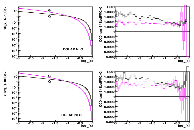
Figure 2: Left frames: the DGLAP evolutions in the NLO approximation from QCDNum16 and EvolFMC (the curves are indistinguishable). Upper curves (magenta and blue): the gluon $xD_{G}(x)$ distr.; lower curves (black and red): the quark $xD_{Q}(x)$ distr. Right frames: the ratio of QCDNum16 to EvolFMC for the gluon (magenta) and quark (black) distributions. Top frames: the evolution up to 10 GeV. Bottom frames: the evolution up to 100 GeV.

In Fig. 2 we show the DGLAP NLO evolution up to 10 GeV and 100 GeV for both the gluon and quark singlet $xD_{f}(x)$ distributions as well as the ratio of the QCDNum16 to EvolFMC results. The QCDNum16 results are based on the extended grid size of $2000\times 600$. The agreement is of the order of $5\div 8\times 10^{-4}$. We will demonstrate in the next subsection that these residual discrepancies are to be attributed to QCDNum16. One has to remember that the comparisons with QCDNum16 are limited to the standard DGLAP evolution only.

6.2 Comparison with semianalytical code APCheb40

It is the most independent test of the EvolFMC code. The semianalytical method of solving the evolution equations used by APCheb40 is entirely different from the MC method and also the library of the evolution kernels is completely independent. At first, in Fig. 3, we show the comparisons for the standard DGLAP NLO evolution (for this comparison we used the older version, 33, of the APCheb code).

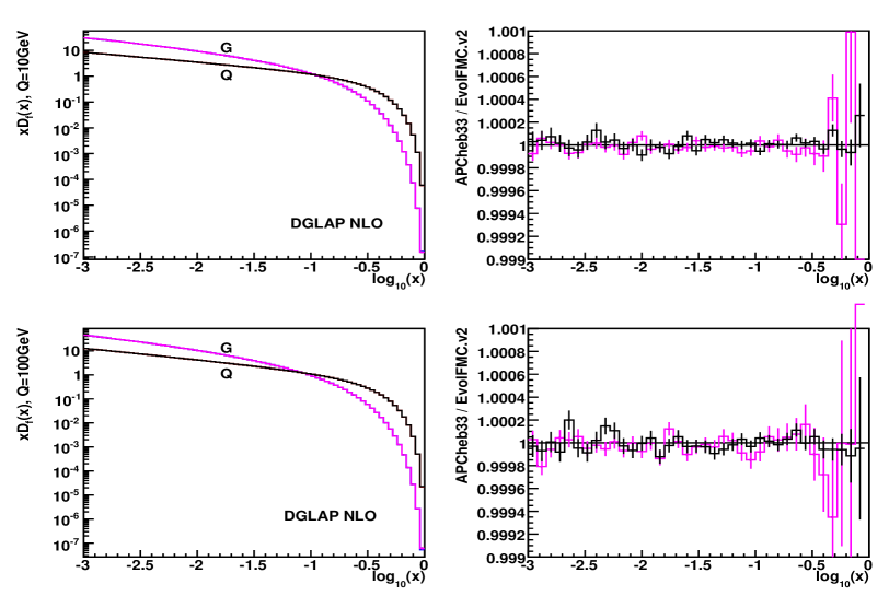
Figure 3: Left frames: the DGLAP evolutions in the NLO approximation from APCheb33 and EvolFMC (the curves are indistinguishable). Upper curves (magenta and blue): the gluon $xD_{G}(x)$ distr.; lower curves (black and red): the quark $xD_{Q}(x)$ distr. Right frames: the ratio of APCheb33 to EvolFMC for the gluon (magenta) and quark (black) distributions. Top frames: the evolution up to 10 GeV. Bottom frames: the evolution up to 100 GeV.

We show the evolution up to 10 GeV and 100 GeV for both the gluon and quark singlet $xD_{f}(x)$ distributions as well as the ratio of the APCheb33 to EvolFMC results. As we see the agreement is remarkable, at the level of $1\times 10^{-4}$, limitted by the statistics. This result clarifies the source of residual disagreement seen in the Fig. 2.

Figure 4: Left frames: the C’-type evolutions in the modified LO approximation from APCheb40 and EvolFMC (the curves are indistinguishable). Upper curves (magenta and blue): the gluon $xD_{G}(x)$ distr.; lower curves (black and red): the quark $xD_{Q}(x)$ distr. Right frames: the ratio of APCheb40 to EvolFMC for the gluon (magenta) and quark (black) distributions. Top frames: the evolution up to 10 GeV. Bottom frames: the evolution up to 100 GeV.

The advantage of APCheb40 over other semianalytical codes, such as QCDNum [8], is that it has the option of the modified-DGLAP evolution built-in, although only at the LO level, see [13] for details. For the sake of comparisons we have modified the LO kernels in APCheb40 in such a way that the coupling constant is implemented in the NLO approximation, whereas the $z$-dependent parts remain in the LO approximation, i.e. the modified kernels are

$$\begin{split}&x\mathcal{K}^{R(B^{\prime})\tt APCheb}_{f^{\prime}f}(t,x,w)=\frac{\alpha_{NLO}(\ln(1-z)+t)}{2\pi}2zP_{f^{\prime}f}^{R(0)}(z)\theta_{1-z>\lambda e^{-t}},\\ &x\mathcal{K}^{R(C^{\prime})\tt APCheb}_{f^{\prime}f}(t,x,w)=\frac{\alpha_{NLO}(\ln(w-x)+t)}{2\pi}2zP_{f^{\prime}f}^{R(0)}(z)\theta_{w-x>\lambda e^{-t}}.\end{split}$$ (20)

In Fig. 4 we show the C’-type evolution up to 10 GeV and 100 GeV for both the gluon and quark singlet $xD_{f}(x)$ distributions as well as the ratio of the APCheb40 to EvolFMC results. The APCheb40 results are based on the interpolation with 100 Chebyshev polynomials. The agreement is again excellent, in most of the $x$-range below $1\times 10^{-4}$.

To summarise, the results of comparison with APCheb40 indicate that technical precision of EvolFMC is much better than our conservative target of $5\times 10^{-4}$.

6.3 Comparison with EvolFMC v.1

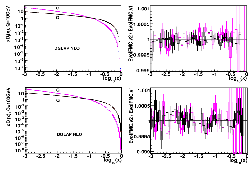
Figure 5: Left frames: the evolutions from EvolFMC v.1 and EvolFMC v.2 (the curves are indistinguishable) for the DGLAP-type NLO evolutions. Upper curves (magenta and blue): the gluon $xD_{G}(x)$ distr.; lower curves (black and red): the quark $xD_{Q}(x)$ distr. Right frames: the ratio of EvolFMC v.2 to EvolFMC v.1 for the gluon (magenta) and quark (black) distributions. Top frames: the evolution up to $Q=10$ GeV. Bottom frames: the evolution up to $Q=100$ GeV.

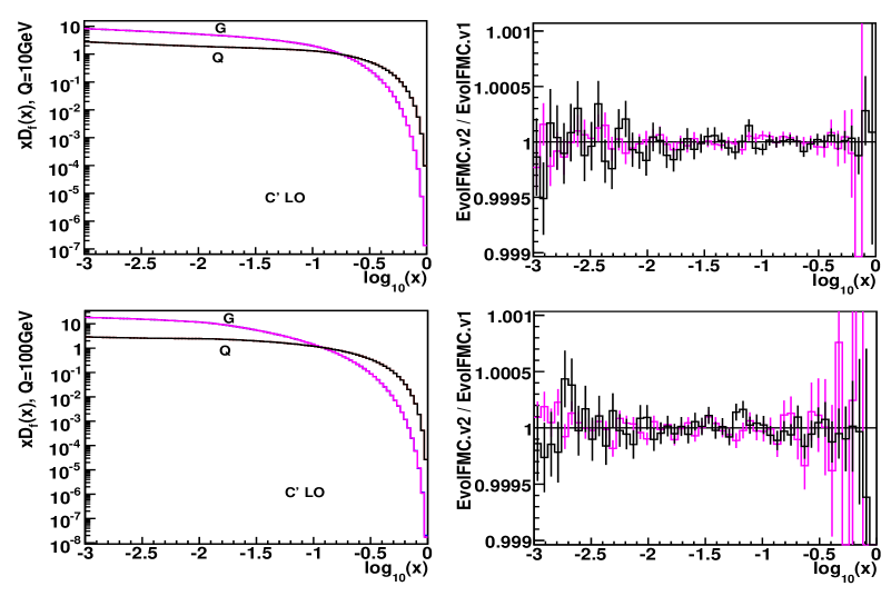
Figure 6: Left frames: the evolutions from EvolFMC v.1 and EvolFMC v.2 (the curves are indistinguishable) for modified-DGLAP C’-type LO evolutions. Upper curves (magenta and blue): the gluon $xD_{G}(x)$ distr.; lower curves (black and red): the quark $xD_{Q}(x)$ distr. Right frames: the ratio of EvolFMC v.2 to EvolFMC v.1 for the gluon (magenta) and quark (black) distributions. Top frames: the evolution up to $Q=10$ GeV. Bottom frames: the evolution up to $Q=100$ GeV.

The old EvolFMC v.1 has been extensively tested both for the DGLAP (up to NLO) and modified-DGLAP (LO only) cases with the overall relative precision tag of about $10^{-3}$ [1, 13]. As an example of the backward compatibility tests we show in Fig.  5 the comparison of EvolFMC v.1 with EvolFMC v.2 for the DGLAP-type NLO evolution and in Fig.  6 for the modified-DGLAP C’-type LO evolution, both up to 10 and 100 GeV. As we can see the results agree within the statistical errors at the level of $5\times 10^{-4}$, as desired.

As we have explained in Introduction, the version v.1 of EvolFMC has different overall structure and organisation of the code as well as different implementation of most of the methods. Therefore this comparison can be regarded as a comparison with an “almost” independent code (for the limited number of evolution types, of course).

6.4 Comparison of different algorithms

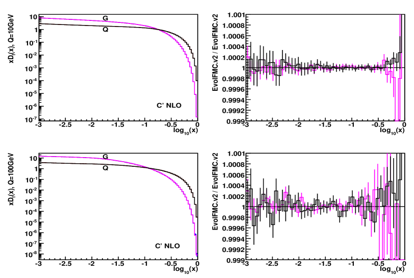
Figure 7: Left frames: the modified-DGLAP C’-type evolutions in NLO approximation from the two algorithms of EvolFMC v.2 (the curves are indistinguishable). Upper curves (magenta and blue): the gluon $xD_{G}(x)$ distr.; lower curves (black and red): the quark $xD_{Q}(x)$ distr. Right frames: the ratio of the two algorithms of EvolFMC v.2 for the gluon (magenta) and quark (black) distributions. Top frames: the evolution up to 10 GeV. Bottom frames: the evolution up to 100 GeV.

In this section we show the tests of the most advanced evolution: of the C’-type in the NLO approximation. We have not found any other code that would solve this type of evolution. For this reason we have implemented in the EvolFMC code the second, auxiliary, MC algorithm that solves this particular type of evolution. The key difference of the auxilliary algorithm with respect to the main algorithm is that the entire NLO correction (including modifications in the argument of the coupling constant) is introduced as a weight and the algorithm itself is based on the LO algorithm described in [28], see [30] for details.

As an example in Fig. 7 we show the comparisons of results of these two NLO algorithms of the C’-type for two evolution time limits: 10 GeV and 100 GeV. As one can see the agreement is well below the level of $5\times 10^{-4}$. This result we consider as the principal test of the NLO C’-type evolution in the code EvolFMC v.2. Of course, the auxiliary algorithm shares with the previous ones a lot of common parts of the code. These common parts however have been extensively tested by all the comparisons described in previous subsections.

We conclude this series of tests with the conservative statement that the EvolFMC v.2 code has the overall technical precision of $5\times 10^{-4}$!

6.5 Weight distributions and speed of algorithms

In Fig. 8 we show the weight distributions for all three main algorithms included in the program EvolFMC v.2. The evolutions are of the NLO type up to 100 GeV.

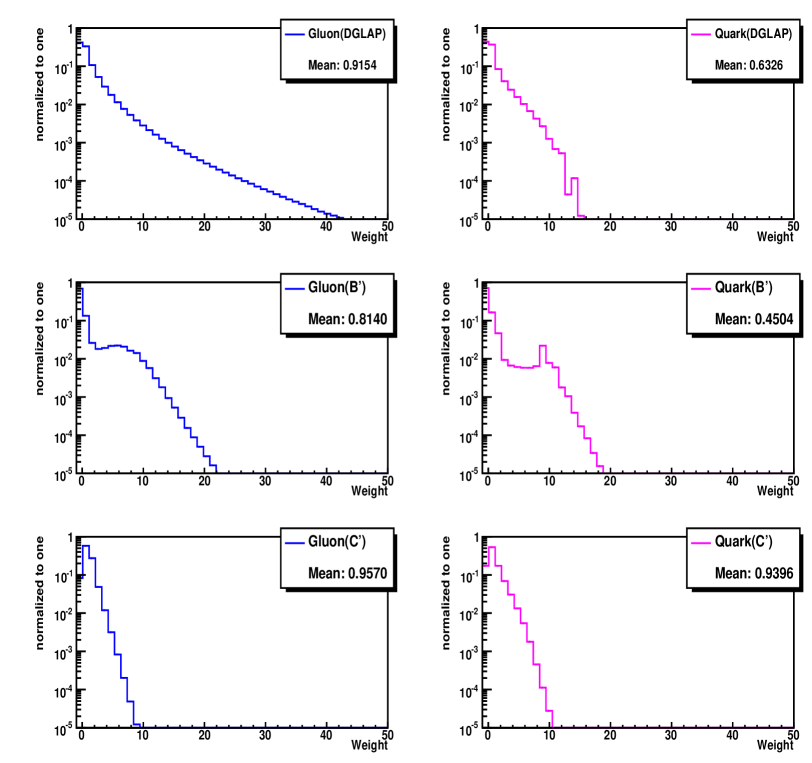
Figure 8: Weight distributions for NLO evolution to 100 GeV (normalized to one). Left frames: gluon. Right frames: quark. Top frames: DGLAP evolution. Central frames: B’-type evolution. Bottom frames: C’-type evolution.

The weights are well behaved and fall down exponentially. The distributions of modified evolutions have shorter tails as compared to the DGLAP case. This is the consequence of the finite IR cut-off used in the modified kernels, as compared to the infinitesimal one used in the DGLAP case. The plots indicate that the conversion to the unweighted events should be quite efficient, especially in the case of moderate target precision level. One has to remember that in the current version of the program we did not perform any additional weight optimization, as we restricted ourselves to the weighted events only. Such an optimization could reduce the tails of the weight distributions even further.

Finally, in Fig. 9 we compare speed of all five algorithms included in the program EvolFMC v.2 both in LO and NLO cases. As we see, despite their complexity and the presence of internal one-dimensional numerical integration, the NLO algorithms are slower only by a factor of few as compared to the very fast LO ones. The slowest one is the B’-type algorithm. Let us note that the algorithms are only partly optimized with respect to speed.

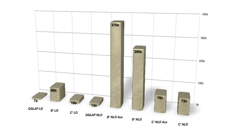
Figure 9: Comparison of the speed of all five algorithms. Plotted times (in seconds) refer to generation of $10^{6}$ events and evolution to 100 GeV. First three blocks illustrate the LO evolution (DGLAP, B’ and C’, respectively), following five blocks the NLO case (DGLAP, B’-auxilary, B’-main, C’-auxiliary and C’-main, respectively).

7 Summary

In this paper we have presented the program EvolFMC v.2. It is a Monte Carlo generator that solves some of the QCD evolution equations for the parton momentum distributions in the weighted event mode. In the current version we have implemented the DGLAP evolution in the LO and NLO approximations and two modified-DGLAP type evolutions. These modifications include the replacement of the argument of the coupling constant by a more complicated functions of the $x$ and $t$ variables. In one case (C’) this function reconstructs the transverse momentum of the emitted partons and in the other case (B’) the approximate transverse momentum. Both of these modified-DGLAP evolutions are implemented in the LO as well as the NLO approximation. The code is written in the C++ language and has the modular structure, easy to extend to additional evolution types. The main limitation of the code is the fact that quarks are treated as massless. We have studied the technical precision of the program by means of extensive comparisons with the non-MC numerical program APCheb40, with the previous version of the code, EvolFMC v.1, and by comparing two independent algorithms for the same evolution implemented in EvolFMC v.2. These tests have proved that the technical precision of the EvolFMC v.2 is at least $5\times 10^{-4}$. To our knowledge it is the first so-precise solution of the QCD evolution equations by means of the Monte Carlo methods.

8 Acknowledgements

Authors would like to thank K. Golec-Biernat and Z. Wa̧s for discussions and comments.

9 Appendix

In this Appendix we list the source code of the simple demo.cxx program from the Demo0 folder.

#include<stdio.h>
#include<math.h>

#include "rndm.h"

#include "bprim_nlo.h"
#include "bprim_lo.h"
#include "bprim_nlo_aux.h"
#include "cprim_lo.h"
#include "cprim_nlo.h"
#include "cprim_nlo_aux.h"
#include "dglap_lo.h"
#include "dglap_nlo.h"

#define DGLAP_LO      0
#define DGLAP_NLO     1
#define CPRIM_LO      2
#define CPRIM_NLO     3
#define CPRIM_NLO_AUX 4
#define BPRIM_LO      5
#define BPRIM_NLO     6
#define BPRIM_NLO_AUX 7

double Lambda         = 0.25;
double numberOfFlavor = 3;
double Qmin           = 1;
double Qmax           = 100;
int TypeOfGenerator   = 0;

rndm * RNgen;
int numberOfEvents = 100;

int main(int argc, char *argv[])
{
Ψif (argc>1)
ΨΨTypeOfGenerator = (atoi(*(++argv))<8) ? atoi(*argv) : 0;

  RNgen = new rndm();
  double T0 = log(Qmin);
  dglap_lo  * dglap_ll
               = new dglap_lo(     T0,Lambda,numberOfFlavor,RNgen);
  dglap_nlo * dglap_nll
               = new dglap_nlo(    T0,Lambda,numberOfFlavor,RNgen);
  CPrim_lo  * cprim_ll
               = new CPrim_lo(     T0,Lambda,numberOfFlavor,RNgen);
  CPrim_nlo * cprim_nll
               = new CPrim_nlo(    T0,Lambda,numberOfFlavor,RNgen);
  CPrim_nlo_aux * cprim_nll_aux
               = new CPrim_nlo_aux(T0,Lambda,numberOfFlavor,RNgen);
  BPrim_nlo * bprim_nlo
               = new BPrim_nlo(    T0,Lambda,numberOfFlavor,RNgen);
  BPrim_lo  * bprim_lo
               = new BPrim_lo(     T0,Lambda,numberOfFlavor,RNgen);
  BPrim_nlo_aux * bprim_nlo_aux
               = new BPrim_nlo_aux(T0,Lambda,numberOfFlavor,RNgen);

Ψdglap_ll->printLogo();

Ψint init_Flavor = 0;
Ψdouble init_Xstart = 1.0;

printf("*******************Starting parameters*****************\n");
Ψprintf("Qmin=%4.2f\n", Qmin);
Ψprintf("Qmax=%4.2f\n", Qmax);
Ψprintf("Type of Equation: %d\n", TypeOfGenerator);
Ψprintf("QCDLambda=%2.4f\n", Lambda);
Ψprintf("numberOfFlavors=%d\n", numberOfFlavor);
Ψprintf("Events to generate:%d\n", numberOfEvents);

printf("*******************Initial Conditions******************\n");
Ψprintf("Flavor: %d\n", init_Flavor);
Ψprintf("Xstart: %1.2f\n", init_Xstart);
printf("*************************Events************************\n");

Ψdouble TStop = log(Qmax);
Ψdouble Tc;

Ψdouble sumwt = 0.0;
Ψdouble sumwt2= 0.0;
Ψint NoEvents =0;

Ψfor (int i=0; i<numberOfEvents; i++)
Ψ{
ΨΨint Flavor = init_Flavor;
ΨΨdouble Xstart = init_Xstart;

ΨΨdouble weight = 1.0;

ΨΨswitch (TypeOfGenerator)
ΨΨ{
ΨΨcase CPRIM_NLO:
ΨΨ        cprim_nll->GenerateEvent(Tc, Xstart, weight, TStop, Flavor);
ΨΨ        break;
ΨΨΨcase CPRIM_NLO_AUX:
ΨΨ        cprim_nll_aux->GenerateEvent(Tc, Xstart, weight, TStop, Flavor);
ΨΨ        break;
ΨΨcase CPRIM_LO:
ΨΨ        cprim_ll->GenerateEvent(Tc, Xstart, weight, TStop, Flavor);
ΨΨ        break;
ΨΨcase DGLAP_LO:
ΨΨ        dglap_ll->GenerateEvent(Tc, Xstart, weight, TStop, Flavor);
ΨΨ        break;
ΨΨΨcase DGLAP_NLO:
ΨΨ        dglap_nll->GenerateEvent(Tc, Xstart, weight, TStop, Flavor);
ΨΨ        break;
ΨΨcase BPRIM_LO:
ΨΨ        bprim_lo->GenerateEvent(Tc, Xstart, weight, TStop, Flavor);
ΨΨ        break;
ΨΨcase BPRIM_NLO:
ΨΨ        bprim_nlo->GenerateEvent(Tc, Xstart, weight, TStop, Flavor);
ΨΨ        break;
ΨΨcase BPRIM_NLO_AUX:
ΨΨ        bprim_nlo_aux->GenerateEvent(Tc, Xstart, weight, TStop, Flavor);
ΨΨ        break;
ΨΨ}
ΨΨsumwt =sumwt + weight;
ΨΨsumwt2=sumwt2 + weight*weight;
ΨΨNoEvents = NoEvents+1;
ΨΨif (NoEvents<100)
ΨΨ{
ΨΨΨprintf("X=%1.6f, weight=%1.6f, flavor=%d\n", Xstart, weight, Flavor);
ΨΨ}
Ψ}
double integral=sumwt/NoEvents;
double error = sqrt( (sumwt2/NoEvents
                   - (sumwt/NoEvents)*(sumwt/NoEvents)) /NoEvents);

printf("***********************Output**************************\n");
printf("\n [sum_f=flavor] [int_eps^1 dx] D_f(x,t)= %1.6f +- %1.6f\n\n"
                                                  ,integral, error);
printf("*******************************************************\n");

return 0;
}

References

- [1] K. Golec-Biernat, S. Jadach, W. Płaczek, and M. Skrzypek, Acta Phys. Polon. B37, 1785 (2006), hep-ph/0603031.
-
[2]
L.N. Lipatov, Sov. J. Nucl. Phys. 20 (1975) 95;
V.N. Gribov and L.N. Lipatov, Sov. J. Nucl. Phys. 15 (1972) 438;
G. Altarelli and G. Parisi, Nucl. Phys. 126 (1977) 298;
Yu. L. Dokshitzer, Sov. Phys. JETP 46 (1977) 64. -
[3]
L.N. Lipatov, Sov. J. Nucl. Phys. 23 (1976) 338;
E.A. Kuraev, L.N. Lipatov and V.S. Fadin, Sov. Phys. JETP 45 (1977) 199;
I.I. Balitsky and L.N. Lipatov, Sov. J. Nucl. Phys. 28 (1978) 822;
L.N. Lipatov, Sov. Phys. JETP 63 (1986) 904. -
[4]
M. Ciafaloni, Nucl. Phys. B296 (1988) 49;
S. Catani, F. Fiorani and G. Marchesini, Phys. Lett. B234 339, Nucl. Phys. B336 (1990) 18;
G. Marchesini, Nucl. Phys. B445 (1995) 49. - [5] B. I. Ermolaev, M. Greco and S. I. Troyan, Acta Phys. Polon. B38 (1986) 2243.
- [6] S. Weinzierl, Comput. Phys. Commun. 148, 314 (2002), hep-ph/0203112.
- [7] M. Miyama and S. Kumano, Comput. Phys. Commun. 94, 185 (1996), hep-ph/9508246.
- [8] M. Botje, QCDNUM16: A fast QCD evolution program, 1977, ZEUS Note 97-066, http://www.nikhef.nl/~h24/qcdcode/.
- [9] A. Chuvakin and J. Smith, Comput. Phys. Commun. 143, 257 (2002), hep-ph/0103177.
- [10] C. Coriano and C. Savkli, Comput. Phys. Commun. 118, 236 (1999), hep-ph/9803336.
- [11] R. Toldra, Comput. Phys. Commun. 143, 287 (2002), hep-ph/0108127.
- [12] K. Golec-Biernat, APCheb40, the Fortran code available on the request from the author, unpublished.
- [13] K. Golec-Biernat, S. Jadach, W. Płaczek, and M. Skrzypek, Acta Phys. Polon. B39, 115 (2008), arXiv:0708.1906 [hep-ph].
- [14] T. Sjostrand, S. Mrenna, and P. Skands, (2007), arXiv:0710.3820 [hep-ph].
- [15] T. Sjostrand et al., Comput. Phys. Commun. 135, 238 (2001), hep-ph/0010017.
- [16] S. Gieseke et al., (2006), hep-ph/0609306.
- [17] G. Corcella et al., JHEP 01, 010 (2001), hep-ph/0011363.
- [18] L. Lonnblad, Comput. Phys. Commun. 71, 15 (1992).
- [19] Y. Kurihara et al., Nucl. Phys. B654, 301 (2003), hep-ph/0212216.
- [20] S. Tsuno, T. Kaneko, Y. Kurihara, S. Odaka, and K. Kato, Comput. Phys. Commun. 175, 665 (2006), hep-ph/0602213.
- [21] J. C. Collins, T. C. Rogers, and A. M. Stasto, Phys. Rev. D77, 085009 (2008), arXiv:0708.2833 [hep-ph].
- [22] Z. Nagy and D. E. Soper, JHEP 09, 114 (2007), arXiv:0706.0017 [hep-ph].
- [23] S. Jadach and M. Skrzypek, (2009), arXiv:0905.1399 [hep-ph].
- [24] M. Slawinska and A. Kusina, (2009), arXiv:0905.1403 [hep-ph].
- [25] Small x Collaboration, B. Andersson et al., Eur. Phys. J. C25, 77 (2002), hep-ph/0204115.
- [26] S. Jadach and M. Skrzypek, Acta Phys. Polon. B35, 745 (2004), hep-ph/0312355.
- [27] W. Płaczek, K. Golec-Biernat, S. Jadach, and M. Skrzypek, Acta Phys. Polon. B38, 2357 (2007), arXiv:0704.3344.
- [28] K. Golec-Biernat, S. Jadach, W. Płaczek, P. Stephens, and M. Skrzypek, Acta Phys. Polon. B38, 3149 (2007), hep-ph/0703317.
- [29] M. Skrzypek, S. Jadach, K. Golec-Biernat, and W. Płaczek, Acta Phys. Polon. B38, 2369 (2007).
- [30] P. Stoklosa, W. Płaczek, and M. Skrzypek, (2008), arXiv:0810.2670 [hep-ph].
- [31] R. G. Roberts, Eur. Phys. J. C10, 697 (1999), hep-ph/9904317.
- [32] G. Curci, W. Furmanski, and R. Petronzio, Nucl. Phys. B175, 27 (1980).
- [33] W. Furmanski and R. Petronzio, Phys. Lett. B97, 437 (1980).
- [34] S. Jadach, W. Płaczek, M. Skrzypek, B. F. L. Ward, and Z. Was, Comput. Phys. Commun. 119, 272 (1999), hep-ph/9906277.
- [35] S. Jadach, W. Płaczek, M. Skrzypek, B. F. L. Ward, and Z. Was, Comput. Phys. Commun. 140, 475 (2001), hep-ph/0104049.
- [36] S. Jadach, W. Płaczek, M. Skrzypek, B. F. L. Ward, and Z. Was, Comput. Phys. Commun. 140, 432 (2001), hep-ph/0103163.
- [37] S. Jadach, W. Płaczek, and B. F. L. Ward, Phys. Lett. B390, 298 (1997), also hep-ph/9608412; The Monte Carlo program BHWIDE is available from http://cern.ch/placzek.
- [38] S. Jadach, W. Płaczek, E. Richter-Was, B. F. L. Ward, and Z. Was, Comput. Phys. Commun. 102, 229 (1997).
- [39] S. Jadach, B. F. L. Ward, and Z. Was, Comput. Phys. Commun. 130, 260 (2000), hep-ph/9912214, Program source available from http://home.cern.ch/jadach/.