Evanescent channels and scattering in cylindrical nanowire heterostructures

Abstract

We investigate the scattering phenomena produced by a general finite-range nonseparable potential in a multi-channel two-probe cylindrical nanowire heterostructure. The multi-channel current scattering matrix is efficiently computed using the R-matrix formalism extended for cylindrical coordinates. Considering the contribution of the evanescent channels to the scattering matrix, we are able to put in evidence the specific dips in the tunneling coefficient in the case of an attractive potential. The cylindrical symmetry cancels the ”selection rules” known for Cartesian coordinates. If the attractive potential is superposed over a non-uniform potential along the nanowire, then resonant transmission peaks appear. We can characterize them quantitatively through the poles of the current scattering matrix. Detailed maps of the localization probability density sustain the physical interpretation of the resonances (dips and peaks). Our formalism is applied to a variety of model systems like a quantum dot, a core/shell quantum ring or a double-barrier, embedded into the nanocylinder.

I Introduction

In the last years, there is an increased interest in studying nanowire-based devices due to their broad application area. They can be used as field-effect transistors (FET) Xiang et al. (2006) or gate-all-around (GAA) FET Bryllert et al. (2006); Yeo et al. (2006); Cho et al. (2008), nanowire resonant tunneling diodes M.T.Bjork et al. (2002); Wensorra et al. (2005), solar cells as integrated power sources for nanoelectronic systems Tian et al. (2007), lasers Qian et al. (2008), and also as qubits Hu et al. (2007). Their structural complexity has progresively increased, and the material composition includes III-V materials but also, so attractive for semiconductor industry, group IV materials.

Description of electrical transport and charge distribution in nanowire-based devices has to be done quantum mechanically, and the most appropriate method for such open systems is the scattering theory. Due to the confinement of the motion inside the nanowire, the electrons are free to move only along the nanowire direction, so that these systems are also called quasi-one-dimensional systems. Since many nanowires have circular cross-sectional shape Bryllert et al. (2006); Yeo et al. (2006); Cho et al. (2008), we present in this work a general method, valid within the effective mass approximation, for solving the three-dimensional (3D) Schrödinger equation with scattering boundary conditions in cylindrical geometries. The azimuthal symmetry suggests to use cylindrical coordinates, with $z$ axis along the nanowire. This reduces the scattering problem to two dimensions: $r$ and $z$ directions. Its solution is found numerically using the R-matrix formalism, Smrčka (1990); Wulf et al. (1998); Onac et al. (2001); Racec and Wulf (2001); Racec et al. (2002); Nemnes et al. (2004, 2005); Wulf et al. (2007); Behrndt et al. (2008) extended for cylindrical coordinates.

An interesting effect in a multi-channel scattering problem is that as soon as the potential is not anymore separable, the channels get mixed. If furthermore the scattering potential is attractive, then it leads to unusual scattering properties, like resonant dips in the transmission coefficient just below the next channel minimum energy. As it was shown analytically for a $\delta$ scattering potential Bagwell (1990) or for point scatterers Exner et al. (1996), and later on for a finite-range scattering potentialGurvitz and Levinson (1993); Nöckel and Stone (1994) the dips are due to quasi-bound-states splitting off from a higher evanescent channel. So that evanescent channels can not be neglected when analyzing scattering in two- or three-dimensional quantum systems. These findings were recently confirmed numerically for a Gaussian-type scatterer Bardarson et al. (2004) and also for a quantum dot or a quantum ringGudmundsson et al. (2005) embedded inside nanowires tailored in two-dimensional electron gas (2DEG).

It is the aim of this work to show that we could find the same features in the case of a cylindrical nanowire. Furthermore, in cylindrical nanowires, due to the three-dimensional (3D) modelling, every magnetic quantum number defines a two-dimensional (2D) scattering problem, with different structure of dips for the same scattering potential. Also, the cylindrical symmetry does not forbid any intersubband transmission, so that we could find dips in front of every plateau in the transmission coefficient. We apply our method to a variety of model systems like quantum dot, quantum ring or double-barrier heterostructure, embedded inside the nanowire.

II Model

We consider a cylindrical nanowire with a constant potential on the surface. Inside the wire the electrons are scattered by a potential of finite extend.

II.1 Scattering problem for the cylindrical geometry

In the effective mass approximation, the envelope function associated to the energy $E$ satisfies a Schrödinger-type equation

$$\left[-\frac{\hbar^{2}}{2\mu}\Delta+V(\mathbf{r})\right]\Psi(\mathbf{r})=E\Psi(\mathbf{r}).$$ (1)

We use the symbol $\mu$ to denote the effective mass of the electrons, while $m$ will denote the magnetic quantum number. As long as there are not split gates on the surface of the nanowire, the potential energy $V(\mathbf{r})$ is rotational invariant

$$V(\mathbf{r})=V(r,z)$$ (2)

and nonseparable in a small region of the structure called scattering region. The $z$-axis was considered along the nanowire as shown in Fig. 1.

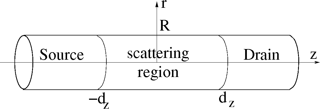
Figure 1: The geometry of the 2D scattering problem.

A scattering potential which does not explicitly depend on the azimuthal angle $\theta$ imposes the eigenfunctions of the orbital angular momentum operator $L_{z}$ as solutions of Eq. (1)

$$\Psi_{m}(E;r,\theta,z)=\frac{e^{im\theta}}{\sqrt{2\pi}}\psi_{m}(E;r,z),$$ (3)

where $m=0,\pm 1,\pm 2,...$ is the magnetic quantum number. This is an integer number due to the requirement that the function $e^{im\theta}$ should be single-valued. The allowed values of the energy $E$ and the functions $\psi_{m}(E;r,z)$ are determined from the equation

$$\begin{split}\left[-\frac{\hbar^{2}}{2\mu}\left(\frac{\partial^{2}}{\partial r^{2}}+\frac{1}{r}\frac{\partial}{\partial r}-\frac{m^{2}}{r^{2}}+\frac{\partial^{2}}{\partial z^{2}}\right)\right.&\left.+V(r,z)\right]\psi_{m}(E;r,z)\\ &=E\psi_{m}(E;r,z).\end{split}$$ (4)

Due to the localized character of the scattering potential it is appropriate to solve Eq. (4) within the scattering theory. In such a way, every magnetic quantum number $m$ defines a two-dimensional (2D) scattering problem. Furthermore, these 2D scattering problems can be solved separately if the scattering potential is rotational invariant. How many of these problems have to be solved, depends on the specific physical quantity which has to be computed.

The potential energy which appears in Eq. (4) has generally two components:

$$V(r,z)=V_{\perp}(r)+V_{scatt}(r,z).$$ (5)

The first one, $V_{\perp}(r)$, describes the lateral confinement of the electrons inside a cylinder of radius $R$ and is translation invariant along the nanowire. We consider a hard wall potential

$$V_{\perp}(r)=\begin{cases}0,&0<r<R\\ \infty,&r\geq R\end{cases}$$ (6)

suitable for modelling either free-standing nanowires or nanowire transistors with no gate leakage current. Both situations correspond to the state-of-the-art devices.

The scattering potential energy inside the nanowire, $V_{scatt}(r,z)$, has generally a nonseparable character in a domain of finite-range and is constant outside this domain. We consider here the nonseparable potential localized within the volume defined by the boundaries $\pm d_{z}$ and $R$, see Fig. 1,

$$V_{scatt}(r,z)=\begin{cases}V_{1},&r\in[0,R],z<-d_{z}\\ V_{s}(r,z),&r\in[0,R],-d_{z}\leq z\leq d_{z}\\ V_{2},&r\in[0,R],z>d_{z}\end{cases}.$$ (7)

There are not material definitions for the planes $z=\pm d_{z}$. Usually, they are chosen inside the highly doped regions of the nanowire characterized by a slowly $z$-varying potential, practically by a constant potential. These regions play the role of the source and drain contacts.

II.2 Scattering states

In the asymptotic regions, $|z|>d_{z}$ i.e. source and drain contacts, the potential energy is separable in the confinement and the transport direction ($V(r,z)=V_{\perp}(r)+V_{s}$) and Eq. (4) can be directly solved using the separation of variables method

$$\psi_{m}(E;r,z)=\phi(r)\varphi(z).$$ (8)

The function $\phi(r)$ satisfies the radial equation

$$-\frac{\hbar^{2}}{2\mu}\left[\frac{d^{2}}{dr^{2}}+\frac{1}{r}\frac{d}{dr}-\frac{m^{2}}{r^{2}}+V_{\perp}(r)\right]\phi(r)=E_{\perp}\phi(r),$$ (9)

while $\varphi(z)$ satisfies the one-dimensional Schrödinger type equation

$$\left[-\frac{\hbar^{2}}{2\mu}\frac{d^{2}}{dz^{2}}+V_{s}\right]\varphi(z)=(E-E_{\perp})\varphi(z),$$ (10)

where $s=1$ stays for the source contact ($z<-d_{z}$) and $s=2$ for the drain contact ($z>d_{z}$).

Due to the electron confinement inside the cylinder of radius $R$, the solutions of Eq. (9) are given in terms of the Bessel functions of the first kind, $J_{m}$,

$$\phi_{n}^{(m)}(r)=\frac{\sqrt{2}}{RJ_{|m|+1}(x_{mn})}J_{m}(x_{mn}r/R),\quad n=1,2,...$$ (11)

where $x_{mn}$ is the $n$th root of $J_{m}(x)$. The eigenfunctions $\phi_{n}^{(m)}(r)$, called transversal modes, form an orthonormal and complete system of functions. The corresponding eigenenergies are

$$E^{(m)}_{\perp n}=\frac{\hbar^{2}}{2\mu}\left(\frac{x_{mn}}{R}\right)^{2},\quad n=1,2,...$$ (12)

and they depend only on the effective mass and the radius of the cylindrical nanowire. It is worth to mention here that $|\phi_{n}^{(m)}(r)|^{2}$ and and $E^{(m)}_{\perp n}$ depend only on $|m|$.

Every transversal mode together with the associated motion on the transport direction defines the scattering channel on each side of the scattering area ($s=1$ for the source contact and $s=2$ for the drain contact). The scattering channels are indexed by $(mns)$ for each $E$.

If the total energy $E$ and the lateral eigenenergy $E^{(m)}_{\perp n}$ are fixed, i.e. for every $E$, $m$ and $n$, there are at most two linearly independent solutions of Eq. (10). In the asymptotic region they are given as a linear combination of exponential functions

$$\varphi_{sn}^{(m)}(z)=\begin{cases}A_{s}e^{ik_{1nm}z}+B_{s}e^{-ik_{1nm}z},&z<-d_{z}\\ C_{s}e^{ik_{2nm}z}+D_{s}e^{-ik_{2nm}z},&z>d_{z}\end{cases}$$ (13)

where $A_{s}$, $B_{s}$, $C_{s}$ and $D_{s}$ are complex coefficients depending on $n$, $m$ and $E$ for each value of $s=1,2$. The wave vector is defined for each scattering channel $(mns)$ as

$$k_{snm}(E)=k_{0}\sqrt{(E-E_{\perp n}^{(m)}-V_{s})/u_{0}},$$ (14)

where $k_{0}=\pi/2d_{z}$ and $u_{0}=\hbar^{2}k_{0}^{2}/2\mu$. In the case of conducting or open channels

$$E-E_{\perp n}^{(m)}-V_{s}\geq 0,$$ (15)

$k_{snm}$ are positive real numbers and correspond to propagating plane waves. For the evanescent or closed channels

$$E-E_{\perp n}^{(m)}-V_{s}<0,$$ (16)

$k_{snm}$ are given from the first branch of the complex square root function, $k_{snm}=i|k_{snm}|$, and describe exponentialy decaying functions away from the scattering region. Thus, the number of the conducting channels, $N_{sm}(E)$, $s=1,2$, $m\geq 0$, is a function of energy, and for a fixed energy $E$ this is the largest value of $n$, which satisfies the inequality (15) for given values of $s$ and $m$.

Each conducting channel corresponds to one degree of freedom for the electron motion through the nanowire and, consequently, there exists only one independent solution of Eq. (4) for a fixed channel $(mns)$ associated with the energy $E$, $\psi^{(s)}_{nm}(E;r,z)$. For describing further on the transport phenomena in the frame of the scattering theory it is convenient to consider this solution as a scattering state, i.e. as a sum of an incoming component on the channel $(mns)$ and a linear combination of outgoing components on each scattering channel. In a convenient formRacec et al. , the scattering function incident from the source contact ($s=1$) is written as

$$\psi^{(1)}_{nm}(E;r,z)=\frac{\theta(N_{1m}(E)-n)}{\sqrt{2\pi}}\begin{cases}e^{ik_{1nm}(z+d_{z})}\phi^{(m)}_{n}(r)+\sum_{n^{\prime}=1}^{\infty}\limits\mbox{${\mathbf{\cal{S}}}$}^{(m)}_{1n^{\prime},1n}(E)e^{-ik_{1n^{\prime}m}(z+d_{z})}\phi^{(m)}_{n^{\prime}}(r),&z<-d_{z}\\ \sum_{n^{\prime}=1}^{\infty}\limits\mbox{${\mathbf{\cal{S}}}$}^{(m)}_{1n,2n^{\prime}}(E)e^{ik_{2n^{\prime}m}(z-d_{z})}\phi^{(m)}_{n^{\prime}}(r),&z>d_{z}\end{cases}$$ (17a)

and the scattering function incident from the drain contact ($$s=2$$) as

$$\psi^{(2)}_{nm}(E;r,z)=\frac{\theta(N_{2m}(E)-n)}{\sqrt{2\pi}}\begin{cases}\sum_{n^{\prime}=1}^{\infty}\limits S^{(m)}_{1n^{\prime},2n}(E)e^{-ik_{1n^{\prime}m}(z+d_{z})}\phi^{(m)}_{n^{\prime}}(r),&z<-d_{z}\\ e^{-ik_{2nm}(z-d_{z})}\phi^{(m)}_{n}(r)+\sum_{n^{\prime}=1}^{\infty}\limits S^{(m)}_{2n^{\prime},2n}(E)e^{ik_{2n^{\prime}m}(z-d_{z})}\phi^{(m)}_{n^{\prime}}(r),&z>d_{z}\end{cases}$$ (17b)

The step functions $\theta$ in the above expressions, with $\theta(x\geq 0)=1$ and $\theta(x<0)=0$, assure that the scattering functions are defined only for conducting channels.

The three-dimensional scattering states, solutions of Eq. (1) for rotational invariant geometries can be now written as

$$\Psi^{(s)}_{nm}(E;r,\theta,z)=\frac{e^{im\theta}}{\sqrt{2\pi}}\psi^{(s)}_{nm}(E;r,z).$$ (18)

Being eigenfunctions of an open system, they are orthonormalized in the general sense Wulf et al. (2007)

$$\int_{-\infty}^{\infty}dz\int_{0}^{R}dr\;r\int_{0}^{2\pi}d\theta\;\Psi_{mn}^{(s)}(E;r,\theta,z)\Psi_{m^{\prime}n^{\prime}}^{(s^{\prime})}(E^{\prime};r,\theta,z)^{*}=\delta_{mm^{\prime}}\delta_{ss^{\prime}}\delta_{nn^{\prime}}\frac{\delta(E-E^{\prime})}{g_{snm}(E)},$$ (19)

where $g_{snm}(E)$ is the 1D density of states, $g_{snm}(E)=\mu/[\hbar^{2}k_{snm}(E)]$.

The physical interpretation of the expressions (17) is that, due to the nonseparable character of the scattering potential, a plane wave incident onto the scattering domain is reflected on every channel - open or closed for transport - on the same side of the system and transmitted on every channel - open or closed for transport - on the other side. The reflection and transmission amplitudes are described by the complex coefficients $S^{(m)}_{sn^{\prime},sn}$ and $S^{(m)}_{s^{\prime}n^{\prime},sn}$ with $s\neq s^{\prime}$, respectively, and all of them should be nonzero. These coefficients define a matrix with $N_{1m}(E)+N_{2m}(E)$ infinite columns. For an elegant solution of the scattering problem we extend $S^{(m)}(E)$ to an infinite square matrix and set at zero the matrix elements without physical meaning, $S^{(m)}_{s^{\prime}n^{\prime},sn}(E)=0$, $n>N_{sm}(E)$, $s=1,2$. In this way we define the wave transmission matrix Bagwell (1990) or the generalized scattering matrix Schanz and Smilansky (1995). This is not the well-known scattering matrix (current transmission matrix) whose unitarity reflects the current conservation. The generalized scattering matrix is a non-unitary matrix, which has the big advantage that it allows for a description of the scattering processes not only in the asymptotic region but also inside the scattering area.

For the sake of simplicity and also considering that for rotational invariant potentials the 2D scattering problems generated by every magnetic quantum number $m$ can be solved separately, the index $m$ will be omitted in the following subsections.

II.3 R-matrix formalism for cylindrical geometry

The scattering functions inside the scattering region are determinated using the R-matrix formalism, i.e. they are expressed in terms of the eigenfunctions corresponding to the closed counterpart of the scattering problem Smrčka (1990); Wulf et al. (1998); Onac et al. (2001); Racec and Wulf (2001); Racec et al. (2002); Nemnes et al. (2004, 2005); Wulf et al. (2007). In our opinion this is a more appropriate method than the common mode space approach which implies the expansion of the scattering functions inside the scattering area in the basis of the transversal modes $\phi_{n}(r)$. As it is shown in Ref. [Nöckel and Stone, 1994,Luisier et al., 2006] the mode space approach has limitations for structures with abrupt changes in the potential or sudden spatial variations in the widths of the wire; it breaks even down for coupling operators that are not scalar potentials, like in the case of an external magnetic field. In the R-matrix formalism the used basis contains all the information about the scattering potential, and this type of difficulties can not appear.

Thus, the scattering functions inside the scattering region are given as

$$\psi_{n}^{(s)}(E;r,z) = \sum_{l=1}^{\infty}a_{ln}^{(s)}(E)\chi_{l}(r,z),$$ (20)

with $r\in[0,R]$ and $z\in[-d_{z},d_{z}]$.

The so-called Wigner-Eisenbud functions, $\chi_{l}(r,z)$, firstly used in the nuclear physics Wigner and Eisenbud (1947); Lane and Thomas (1958), satisfy the same equation as $\psi_{n}^{(s)}(r,z)$, Eq. (4), but with different boundary conditions in the transport direction: Since the scattering function $\psi_{n}^{(s)}(r,z)$ satisfies energy dependent boundary conditions derived from Eq. (17) due to the continuity of the scattering function and its derivative at $z=\pm d_{z}$, the Wigner-Eisenbud function $\chi_{l}(r,z)$ has to satisfy Neumann boundary conditions at the interfaces between the scattering region and contacts, $\left.\partial\chi_{l}/\partial z\right|_{z=\pm d_{z}}=0$, $l\geq 1$. The infinite potential outside the nanowire requires Dirichlet boundary condition on the cylinder surface for the both functions, $\psi_{n}^{(s)}(R,z)=0$ and $\chi_{l}(R,z)=0$. The functions $\chi_{l}$, $l\geq 1$, built a basis which verifies the orthogonality- and the closure- relation. The corresponding eigenenergies to $\chi_{l}$ are denoted by $E_{l}$ and are called Wigner-Eisenbud energies. Since the Wigner-Eisenbud problem is defined on a closed volume with self-adjoint boundary conditions, the eigenfunctions $\chi_{l}$ and the eigenenergies $E_{l}$ can be choosen as real quantities. The Wigner-Eisenbud problem is, thus, the closed counterpart of the scattering problem.

In the case of the one-dimensional system it was recently proven mathematically rigorous that the R-matrix formalism allows for a proper expansion of the scattering matrix on the real energy axisBehrndt et al. (2008). In this section we present an extension of the R-matrix formalism for 2D scattering problem with cylindrical symmetry.

To calculate the expansion coefficients $a_{ln}^{(s)}(E)$ we multiply Eq. (4) by $\chi_{l}(r,z)$ and the equation satisfied by the Wigner-Eisenbud functions by $\psi_{n}^{(s)}(E;r,z)$. The difference between the resulting equations is integrated over $[-d_{z},\;d_{z}]\times[0,R]$, and one obtains on the right hand side the coefficient $a_{ln}^{(s)}(E)$. After an integration by parts in the kinetic energy term and using the boundary conditions one finds $a_{ln}^{(s)}$ and feed in it into Eq. (20). So, the scattering functions inside the scattering region ($z\in[-d_{z},d_{z}],\;r\in[0,R]$) are obtained in terms of their derivatives at the edges of this domain,

$$\begin{split}\psi_{n}^{(s)}(E,r,z)=\frac{2d_{z}}{\pi}\int_{0}^{R}dr^{\prime}\;r^{\prime}\left[R(E,r^{\prime},-d_{z},r,z)\left.\frac{\partial\psi_{n}^{(s)}(E,r^{\prime},z^{\prime})}{\partial z^{\prime}}\right|_{z^{\prime}=-d_{z}}\right.-\left.R(E,r^{\prime},d_{z},r,z)\left.\frac{\partial\psi_{n}^{(s)}(E,r^{\prime},z^{\prime})}{\partial z^{\prime}}\right|_{z^{\prime}=d_{z}}\right],\end{split}$$ (21)

where the R-function is defined as

$$R(E,r,z,r^{\prime},z^{\prime})\equiv\frac{\hbar^{2}}{2\mu}\sum_{l=1}^{\infty}\frac{\chi_{l}(r,z)\chi_{l}(r^{\prime},z^{\prime})}{E-E_{l}}\frac{\pi}{2d_{z}}.$$ (22)

The functions $\partial\psi_{n}^{(s)}/\partial z$ at $z=\pm d_{z}$ are calculated from the asymptotic form (17) based on the continuity conditions for the derivatives of the scattering functions on the interfaces between the scattering region and contacts.

With these results the scattering functions inside the scattering domain are expressed in terms of the wave transmission matrix $\mathbf{S}$

$$\vec{\Psi}(E;r,z)=\frac{i}{\sqrt{2\pi}}\mathbf{\Theta}(E)[{\bf 1}-\mathbf{S}^{T}(E)\\ \mathbf{K}(E)\vec{R}(E;r,z)],$$ (23)

where the component $(sn)$ of the vector $\vec{\Psi}$ is the scattering function $\psi_{n}^{(s)}(E;r,z)$, $n\geq 1$, $s=1,2$ and $\mathbf{S}^{T}$ denotes the matrix transpose. The diagonal matrix $\mathbf{K}$ has on its diagonal the wave vectors (14) of each scattering channel

$$\mathbf{K}_{sn,s^{\prime}n^{\prime}}(E)=\frac{k_{sn}(E)}{k_{0}}\,\delta_{nn^{\prime}}\delta_{ss^{\prime}},$$ (24)

$n,n^{\prime}\geq 1$, $s,s^{\prime}=1,2$, and the vector $\vec{R}(E;r,z)$ as

$$\vec{R}(E;r,z)=\frac{u_{0}}{\sqrt{k_{0}}}\sum_{l=1}^{\infty}\frac{\chi_{l}(r,z)\vec{\chi}_{l}}{E-E_{l}},$$ (25)

where $\vec{\chi}_{l}$ is a vector with the components

$$(\vec{\chi}_{l})_{sn}=\frac{1}{\sqrt{k_{0}}}\int_{0}^{R}\;\chi_{l}(r,(-1)^{s}d_{z})\phi_{n}(r)rdr,$$ (26)

$n\geq 1,s=1,2$. The diagonal $\mathbf{\Theta}$-matrix, $\mathbf{\Theta}_{sn,s^{\prime}n^{\prime}}(E)=\theta(N_{s}(E)-n)\,\delta_{ss^{\prime}}\,\delta_{nn^{\prime}}$, $n\geq 1$, $s=1,2$, assures non-zero values only for the scattering functions corresponding to the conducting channels.

Using further the continuity of the scattering functions on the surface of the scattering area and expanding $\vec{R}(E;\pm d_{z},r)$ in the basis $\left\{\phi_{n}(r)\right\}_{n\geq 1}$ we find the relation between matrixes $\mathbf{S}$ and $\mathbf{R}$

$$\mathbf{S}(E)=\left[\mathbf{1}-2\left(\mathbf{1}+i\mathbf{R}(E)\mathbf{K}(E)\right)^{-1}\right]\mathbf{\Theta}(E),$$ (27)

with the $\mathbf{R}$-matrix given by means of a dyadic product

$$\mathbf{R}(E)=u_{0}\sum_{l=1}^{\infty}\frac{\vec{\chi}_{l}\,\vec{\chi}_{l}^{T}}{E-E_{l}}.$$ (28)

According to the above relation, $\mathbf{R}$ is an infinite-dimensional symmetrical real matrix. The above form allows for a very efficient numerical implementation for computing the $\mathbf{R}$-matrix.

The expression (27) of the $\mathbf{S}$-matrix in terms of the $\mathbf{R}$-matrix is the key relation for solving 2D scattering problems using only the eigenfunctions and the eigenenergies of the closed system. On the base of Eq. (27) the wave transmission matrix is calculated and after that the scattering functions in each point of the system are obtained using Eqs. (17) and (23).

To come back to the dependence on $m$, we point out that the Wigner-Eisenbud functions and energies are $m$-dependent, so that the matrixes $\mathbf{R}$, $\mathbf{K}$ and $\mathbf{\Theta}$ and the vector $\vec{\Psi}(E;r,z)$ are $m$-dependent in relations (27) and (23).

II.4 Reflection and transmission coefficients

Using the density current operator

$$\mathbf{j}(\mathbf{r})=\frac{\hbar}{2i\mu}\Bigl{(}\Psi(\mathbf{r})\nabla\Psi(\mathbf{r})^{*}-\Psi(\mathbf{r})^{*}\nabla\Psi(\mathbf{r})\Bigr{)},$$ (29)

one can define, as usually, the transmission and reflection probabilities. Büttiker et al. (1985) $\Psi(\mathbf{r})^{*}$ denotes the complex conjugate of the scattering wave function (18).

The $r$-component of the density current $j_{r}(r,\theta,z)$ is zero in leads, because $\phi_{n}(r)$ are real functions. The component $\theta$ of the incident density current is $m$ dependent,

$$(j_{inc}(r,\theta,z))_{\theta}=\frac{\hbar^{2}}{\mu}\frac{1}{(2\pi)^{2}}\frac{1}{r}m|\phi_{n}(r)|^{2},$$

so that if one sums over all $m$ values, then they cancel each other. This is also valid for the reflected and transmitted current fluxes. What remains is the $z$-component of the particle density current $j_{z}(r,\theta,z)$, which integrated over the cross section of the nanocylinder with the corresponding measure, $rdr$, provides the very well known relations for the transmission and reflection probabilities. The probability for an electron incident from source, $s=1$, on channel $n$ to be reflected back into source on channel $n^{\prime}$ is

$$R_{nn^{\prime}}^{(1)}=\frac{k_{1n^{\prime}}}{k_{1n}}|S_{1n,1n^{\prime}}^{t}|^{2},$$ (30)

and the probability to be tranmitted into drain, $s=2$, on channel $n^{\prime}$ is

$$T_{nn^{\prime}}^{(1)}=\frac{k_{2n^{\prime}}}{k_{1n}}|S_{1n,2n^{\prime}}^{t}|^{2}.$$ (31)

The reflection and transmission probabilities for evanescent (closed) channels are zero. The total transmission and reflection coefficients for an electron incident from reservoir $s=1$ are defined as

$$T^{(1)}=\sum_{n,n^{\prime}}T^{(1)}_{nn^{\prime}},\quad R^{(1)}=\sum_{n,n^{\prime}}R^{(1)}_{nn^{\prime}}.$$ (32)

More detailed properties of the many-channel tunneling and reflection probabilities are given in Ref. [Büttiker et al., 1985], but note that our indexes are interchanged with respect to the definitions used there. Of course, all these coefficients are $m$-dependent.

II.5 Current scattering matrix

Further, we define the energy dependent current scattering matrix as

$${\tilde{\mathbf{S}}}(E)=\mathbf{K}^{1/2}(E)\mathbf{\Theta}(E)\mathbf{S}(E)\mathbf{K}^{-1/2}(E),$$ (33)

so that its elements give directly the reflection and transmission probabilities

$$|\tilde{S}_{1n^{\prime},1n}(E)|^{2} =R_{nn^{\prime}}^{(1)}(E), |\tilde{S}_{2n^{\prime},2n}(E)|^{2} =R_{nn^{\prime}}^{(2)}(E),$$ (34)

$$|\tilde{S}_{2n^{\prime},1n}(E)|^{2} =T_{nn^{\prime}}^{(1)}(E), |\tilde{S}_{1n^{\prime},2n}(E)|^{2} =T_{nn^{\prime}}^{(2)}(E).$$ (35)

The diagonal $\mathbf{\Theta}$-matrix assures that the matrix elements of $\tilde{\mathbf{S}}$ are nonzero only for the conducting channels, for which the transmitted flux is nonzero. Using the $\mathbf{R}$-matrix representation of $\mathbf{S}$, Eq. (27), we find from the above relation

$${\tilde{\mathbf{S}}}(E)=\mathbf{\Theta}(E)\left[\mathbf{1}-2(\mathbf{1}+i\mathbf{\Omega}(E))^{-1}\right]\mathbf{\Theta}(E),$$ (36)

with the infinite dimensional matrix $\mathbf{\Omega}$

$$\mathbf{\Omega}(E)=u_{0}\sum_{l=1}^{\infty}\frac{\vec{\alpha}_{l}\,\vec{\alpha}^{T}_{l}}{E-E_{l}}=\mathbf{K}^{1/2}(E)\mathbf{R}(E)\mathbf{K}^{1/2}(E)$$ (37)

and the column vector

$$\vec{\alpha}_{l}(E)=\mathbf{K}^{1/2}(E)\,\vec{\chi}_{l},$$ (38)

with $l\geq 1$. According to the definition (37) the matrix $\mathbf{\Omega}$ is a symmetrical one, $\mathbf{\Omega}=\mathbf{\Omega}^{T}$, and from Eq. (36) it follows that ${\tilde{\mathbf{S}}}$ also has this property, ${\tilde{\mathbf{S}}}={\tilde{\mathbf{S}}}^{T}$. On this basis one can demonstrate that the tunneling coefficient characterizes one pair of open channels irrespective of the origin of the incident flux $T^{(1)}_{nn^{\prime}}=\left|{\tilde{S}}_{2n^{\prime},1n}\right|^{2}=\left|{\tilde{S}}_{1n,2n^{\prime}}\right|^{2}=T^{(2)}_{n^{\prime}n}$. This is a well-known property of the transmission through a scattering system and it shows that the current scattering matrix used here is properly defined. The restriction of $\tilde{\mathbf{S}}$-matrix to the open channels is the well known current scattering matrix Wulf et al. (1998); Racec and Wulf (2001); Racec et al. (2002), commonly used in the Landauer-Büttiker formalism. For a given energy $E$ this is a $(N_{1}+N_{2})\times(N_{1}+N_{2})$ matrix which has to satisfy the unitarity condition, according to the flux conservation.

The relation (36) is the starting point for a resonance theory Racec and Wulf (2001); Racec et al. , which allows for an explicit analytical expression for the transmission peak as a Fano resonance with a complex asymmetry parameter.

In the numerical computations, the matrixes $\mathbf{S}$, $\mathbf{R}$, $\mathbf{\Omega}$, $\tilde{\mathbf{S}}$ and $\mathbf{\Theta}$ have the dimension $2N\times 2N$, and the vectors $\vec{\chi}_{l}$, $\vec{\alpha}_{l}(E)$ have $2N$ components, where $N$ is the number of scattering channels (open and closed) taken numerically into account. The number of the Wigner-Eisenbud functions and energies computed numerically establishes the maximum value for the index $l$.

III Cylindrical nanowire heterostructure model systems

The formalism presented above is general and can be applied to a variety of the cylindrical nanowire heterostructures. We consider a series of heterostructures embedded in an infinite cylindrical nanowire of radius $R=5$nm and effective mass $\mu=0.19m_{0}$ (corresponding to transverse mass in Silicon). We set in all our computations $d_{z}=16$nm, see Fig. 1, and the total number of channels (open and closed) $N=8$. In our calculations, the results do not change if more channels are added.

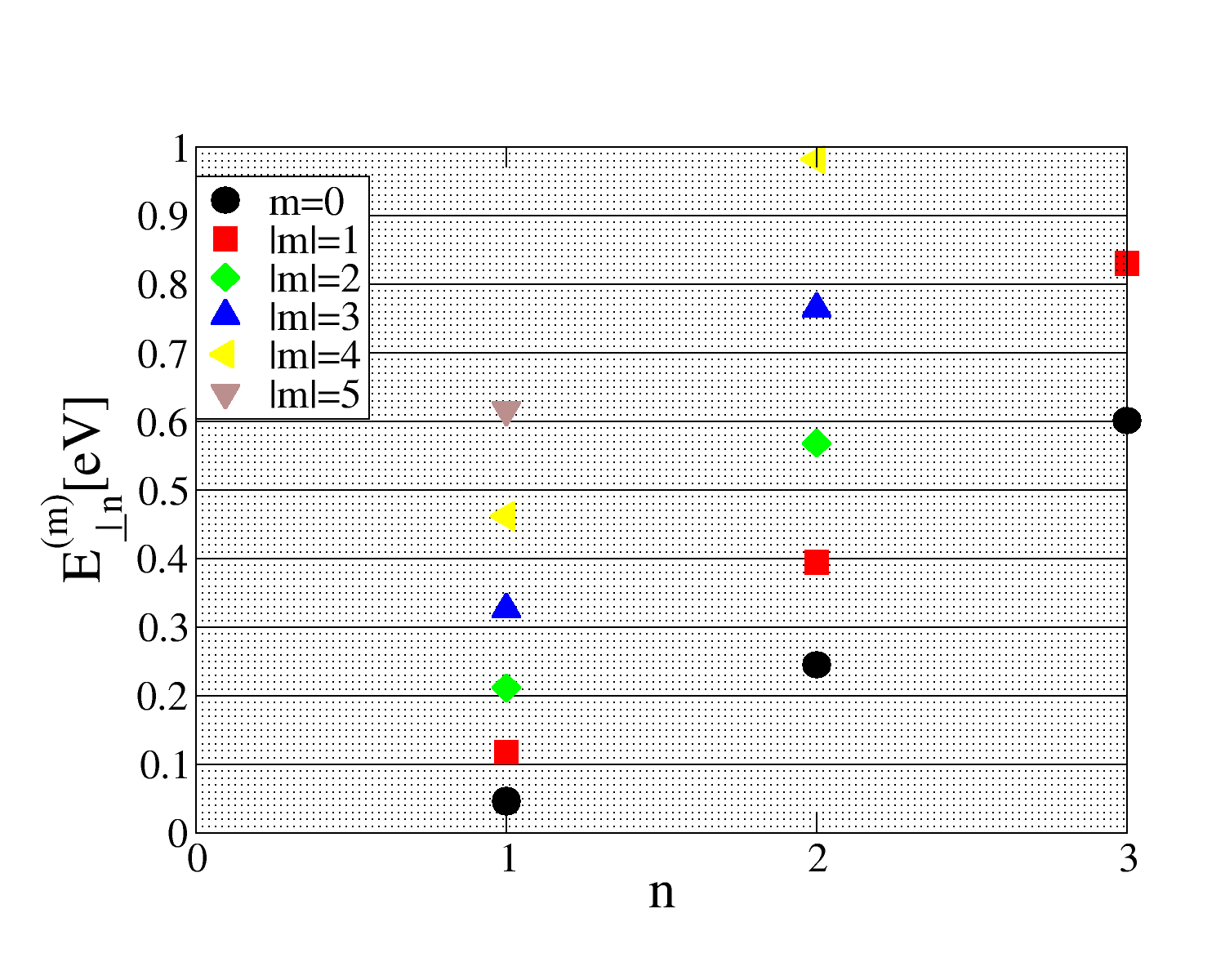
Figure 2: (color online) Energies $E^{(m)}_{\perp,n}$ of the transversal modes for a cylinder with $R=5$nm and $\mu=0.19m_{0}$.

In Fig. 2 are plotted the energies of the transversal modes $E^{(m)}_{\perp,n}$ until $1eV$, for different magnetic quantum numbers $m$, according to (12). The difference between two successive energies of the transversal modes is $m$-dependent, due to the roots $x_{mn}$ of the Bessel functions $J_{m}$.

III.1 Quantum dot embedded into the nanocylinder

III.1.1 Same radius as the host cylinder

In Fig. 3 is sketched a cylindrical quantum dot embedded into a cylindrical nanowire with the same radius. This kind of structures and even compositionally modulated, called also ”nanowire superlattice” Gudiksen et al. (2002), are already realized technologically on different materials basis, as is summarized in a recent review article Shen et al. (2008).

Depending on the band-offsets between the dot material and the host material the potential produced by the dot can be repulsive, yielding a quantum barrier, or attractive, yielding a quantum well. As it is mentioned in Ref. [Gudiksen et al., 2002] the interfaces between the dot and the host material may be considered sharp for nanowires with diameter less than $20$nm. We consider here that the dot yields an attractive potential $V(r,z)$, represented in Fig. 3 by a rectangular quantum well of depth $W_{b}=-0.5eV$ and width $w=8$nm.

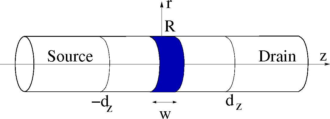
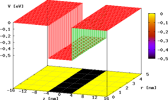
Figure 3: (color online) (a) Sketch of a cylindrical quantum dot embedded into a nanowire with the same radius. We consider that the dot yields an attractive potential $V(r,z)$, represented in (b) by a rectangular quantum well of depth $W_{b}=-0.5eV$ and width $w=8$nm.

The total tunneling coefficient $T^{(1)}$ versus the incident energy $E$ is plotted in Fig. 4, for different magnetic quantum numbers $m$ and different quantum well depths $W_{b}$.

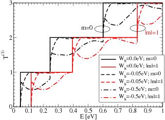
Figure 4: (color online) Total tunneling coefficient as a function of incident energy $E$ for the scattering potential represented in Fig. 3, for different magnetic quantum numbers $m$ and various values of the well depth $W_{b}=0.0eV$ (continuous line), $W_{b}=0.05eV$ (dashed line), and $W_{b}=0.5eV$ (dot-dashed line).

In the absence of the quantum well, $W_{b}=0.0eV$, one can recognize the abrupt stepsvan Wees et al. (1988) in the tunneling coefficient. The transmission increases with a unity, every time a new channel $E^{(m)}_{\perp,n}$ becomes available for transport, i.e. becomes open. The length of the plateaus is given by the difference between two successive transversal mode energies, which differ for different $m$ values. Due to the almost square dependence of the transverse energy levels on the channel number, the length of the plateaus increases. Increasing the depth of the well, deviations from the step-like transmission appear. There are no effects due to the influence of the evanescent channelsGudmundsson et al. (2005), because the scattering potential for this configuration remains furthermore separable in the confinement and the transport direction, $V(r,z)=U(r)+W(z)$.

The spectral representation of the 2D Hamiltonian in this situation is a superposition of the spectrum of each channel, without being perturbed by channel mixing. Considering an attractive potential in $z$-direction, there is always at least one bound state Simon (1976); Klaus (1977) below the continuum spectrum for every channel $n$, see Fig. 7(a)(a). In turn, the bound states of the higher channels $n$ get embedded in the continuous part of the lower channels, forming bound states in continuum (BIC). Since the potential is separable, there is no mix of states, and the BIC states can not be seen as scattering states.

III.1.2 Surrounded by host material

Further we study a cylindrical dot embedded into the nanocylinder, but whose radius $R^{\prime}$ is smaller than the cylinder radius $R$, so that the dot gets surrounded by the host material, see Fig. 5. We consider here again the case that the dot yields an attractive potential, i.e. a rectangular quantum well, plotted in Fig. 5.

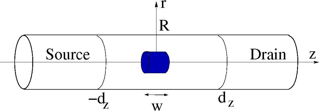
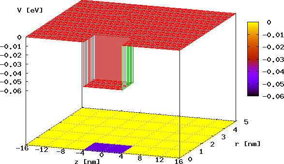
Figure 5: (color online) a) Sketch of a cylindrical quantum dot embedded into the nanocylinder and surrounded by the host material. We consider that the dot yields an attractive potential $V(r,z)$, represented in b) by a rectangular quantum well of depth $W_{b}=-0.05eV$ and width $w=8$nm. The radius of the dot is $R^{\prime}=1$nm.

Even we have chosen a small value for the depth of the quantum well, $W_{b}=-0.05eV$, there are significant deviations in the tunneling coefficient from the step like characteristic, see Fig. 6. Just before a new channel gets open, below $E^{(m)}_{\perp,n}$, there is a dip, i.e. sharp drop, in the tunneling coefficient. These dips are owing to modification of the tunneling coefficient due to the evanescent (closed) channelsBagwell (1990). This is a multichannel effect that was until now studied only in Cartesian coordinates for quantum wires tailored in two-dimensional electron gas Bagwell (1990); Gurvitz and Levinson (1993); Nöckel and Stone (1994); Bardarson et al. (2004); Gudmundsson et al. (2005).

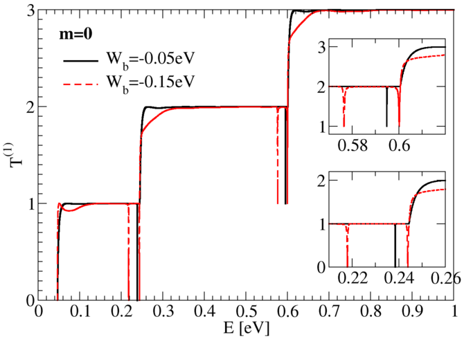
(a) $m=0$

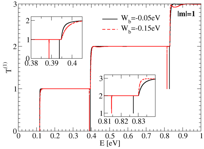
(b) $|m|=1$

Figure 6: (color online) Total tunneling coefficient as a function of total incident energy $E$ for different magnetic quantum numbers $m$ for a cylindrical dot surrounded by the host material as in Fig. 5. A detailed view around the channel minima is presented in the insets.

The dips can be understood considering the simple couple mode model Bagwell (1990); Gurvitz and Levinson (1993); Nöckel and Stone (1994).

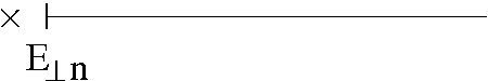
(a) For a channel $n$

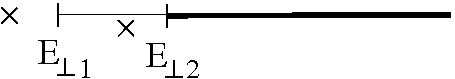
(b) For 2D Hamiltonian, for the first two channels

Figure 7: Sketch of the energy spectrum.

For a dot surrounded by host material, the scattering potential $V(r,z)$ is not anymore separable, so that the scattering mixes the channels Bagwell (1990); Gurvitz and Levinson (1993); Nöckel and Stone (1994). As soon as the scattering potential is attractive, the diagonal coupling matrix element

$$V_{nn}(z)=\int_{0}^{R}\phi_{n}(r)V(r,z)\phi_{n}(r)rdr<0$$ (39)

acts for every channel $n$ as an effective one-dimensional (1D) attractive potential Gurvitz and Levinson (1993), which always allows for at least one bound state Simon (1976); Klaus (1977) below the threshold of the continuum spectrum. We have sketched in Fig. 7(a) the energy spectrum of a channel $n$: the continuous part represented by continuous line is real and starts at $E^{(m)}_{\perp,n}$; the bound state represented by a cross (we consider for simplicity only one), is also real but just below the threshold. By mixing the channels, this bound state becomes a quasi-bound state or resonance, i.e with complex energy, whose real part gets embedded into continuum spectrum of the lower channel, and the imaginary part describes the width of the resonance. The spectrum of the 2D scattering problem is a superposition of the above discussed spectra and is sketched in Fig. 7(b) for spectra corresponding to channels $1$ and $2$. These resonances can be seen now as dips in the tunneling coefficient. The energy difference between the position of the dips and the next subband minima $E^{(m)}_{\perp,n}$ gives the quasi-bound state energy. The positions of the dips, i.e. the quasi-bound state energy, depend on the channel number $n$ and on the magnetic quantum number $m$ and, of course, on the detailed system parameters. In Cartesian coordinates the specific symmetry of the channels (odd and even) do not allow for dips in the first plateauBardarson et al. (2004). In the cylindrical geometry this symmetry is broken, so that we obtain a dip in front of every plateau. Our numerical method allows for high energy resolution in computing the tunneling coefficient, so that we were able to find the dips also in front of higher-order plateaus.

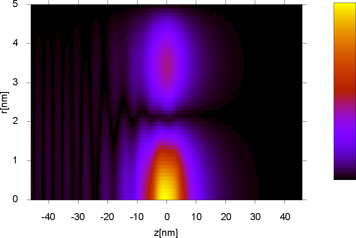
(a) $E=0.238eV$, $n=1$

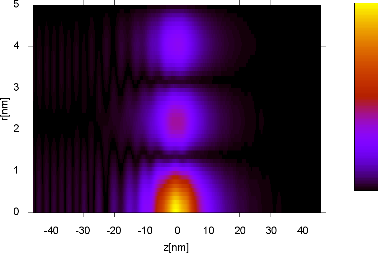
(b) $E=0.594eV$, $n=2$

Figure 8: (color online) Localization probability density, $|\psi^{(1)}_{n}(E,r,z)|^{2}$, for an electron with $m=0$, incident from reservoir $s=1$ into channel $n$ and with total energy $E$, both indicated in the captions. The energies are the dips in Fig. 6(a).

Further insight about the quasi-bound states of the evanescent channels can be gained looking at the wave functions, whose square absolute value $|\psi^{(s)}_{n}(E,r,z)|^{2}$ gives the localization probability density. Considering that the scattering states are orthonormalized in the general sense, the more appropriate quantity to analize would be the local density of states

$$g(E,r)=|\psi^{(s)}_{n}(E,r,z)|^{2}g_{snm}(E),$$ (40)

which differs from the localization probability density just by 1D density of states. For this reason we plot the localization probability density in arbitrary units.

Our numerical implementation based on the R-matrix formalism allows us to produce high resolution maps of the wave functions inside the scattering region, see Eq. (23). In Figs. 8, 9 is represented the localization probability density $|\psi^{(1)}_{n}(E,r,z)|^{2}$ of an electron, incident from source ($s=1$) and has a total energy corresponding to the dips in Fig. 6. The total energy $E$ and the channel $n$, on which the electron is incident, are specified at every plot. Let discuss Fig. 8(a). The total energy $E=0.238eV$ is less than the energy of the second transversal mode, $E_{\perp,2}^{(0)}=0.244eV$, so that only first channel is open, thus the incident wave from the source contact is node-less in $r$-direction. But, as it can be seen in Fig. 8(a), the scattering wave function inside the scattering region has a node in the $r$-direction, i.e. position in $r$ where the wave function is zero. This means that the wave function corresponds to the quasi-bound state splitting off from the second transversal mode, which is an evanescent one. The quasi-bound state is reachable now in a scattering formulation due to channel mixing. The wave function has a pronounced peak around the scattering potential, i.e. $z\in[-4,4]$nm, which decreases exponentially to the left and to the right. To the left of the scattering potential one observes the interference pattern produced by the incident wave and the reflected one, while to the right only the transmitted part exists.

The wave function considered in Fig. 8(b) has the energy less than the third transversal channel, $E^{(0)}_{\perp,3}=0.6006eV$, so that the incident part of the scattering state on the second mode $n=2$ has one node in $r$-direction. But the scattering function shows inside the scattering region two nodes in the $r$-direction, so it corresponds to a quasi-bound state splitting off from the above evanescent channel, the third one.

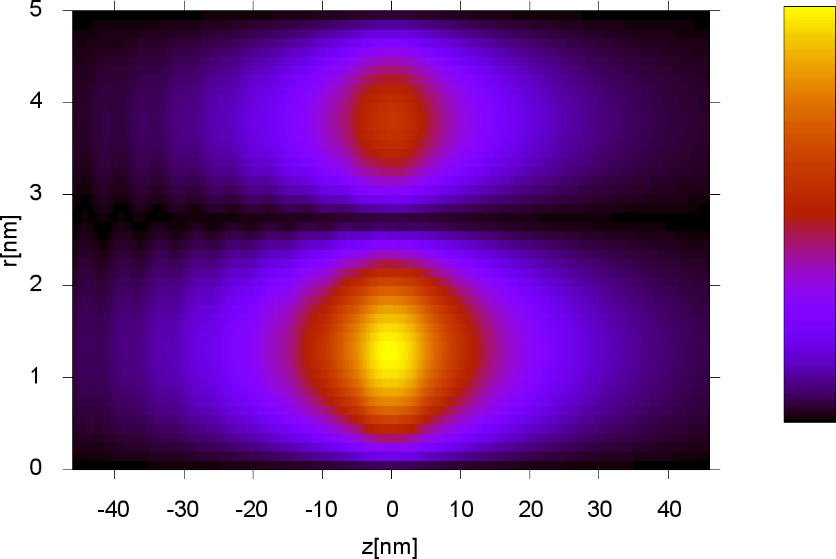
(a) $E=0.393eV$, $n=1$

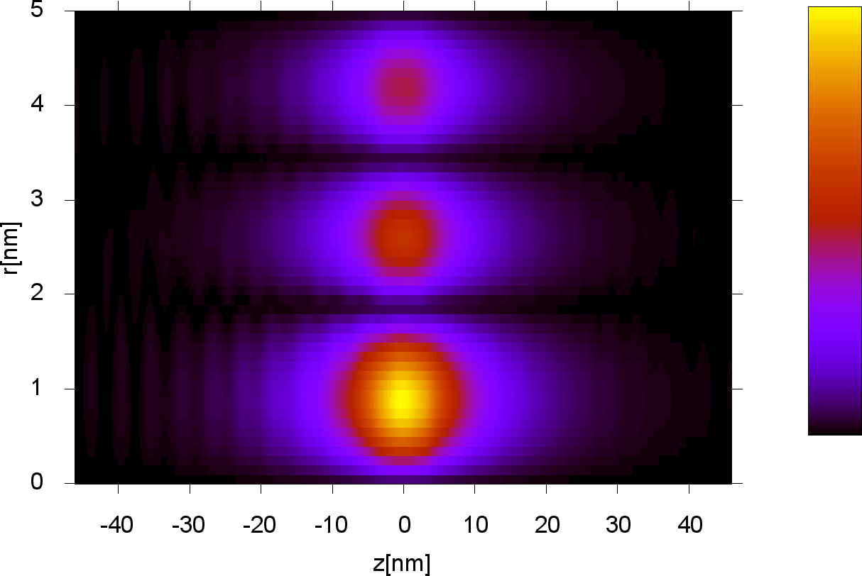
(b) $E=0.827eV$, $n=2$

Figure 9: (color online) Localization probability density $|\psi^{(1)}_{nm}(E,r,z)|^{2}$ for an electron, with $|m|=1$, incident from reservoir $s=1$ into channel $(nm)$ and with total energy $E$, indicated in the captions. The energies are the dips in Fig. 6(b) for $W_{b}=-0.05eV$.

One gets similar pictures for all $m$-values, with the difference that for $m\not=0$ the wave functions are zero for $r=0$, like it is shown in Fig. 9 for the case $|m|=1$. In Figs. 8 and 9 one can observe that the transmitted part of the scattering wave function is zero, in agreement with the resonant backscattering specific to the quasi-bound states of the evanescent channels Bagwell (1990); Gurvitz and Levinson (1993).

The extension of the quasi-bound state of an evanescent channel is given outside the scattering region by the exponential decaying functions $\exp[\kappa_{1nm}(z+d_{z})]$ for $z>-d_{z}$ and $\exp[-\kappa_{2nm}(z-d_{z})]$ for $z<d_{z}$, where $\kappa_{snm}=i|k_{snm}|$ and $k_{snm}$ is defined in (14). This means, the closer the resonance to the threshold of the evanescent channel $E^{(m)}_{\perp,n}$, the slower the exponential function decreases, yielding long exponential tails into the leads. This can be clearly seen for the quasi-bound state represented in Fig. 9(a), whose quasi-bound state is just $0.92meV$ below the subband minimum $E^{(1)}_{\perp,2}=0.394eV$, see Fig. 6(b). Since the localization probability density enters the quantum calculation of the charge distribution one gets difficulties in setting the correct boundaries for the Hartree calculations, i.e. Schrödinger-Poisson system. This has to be studied in a future work.

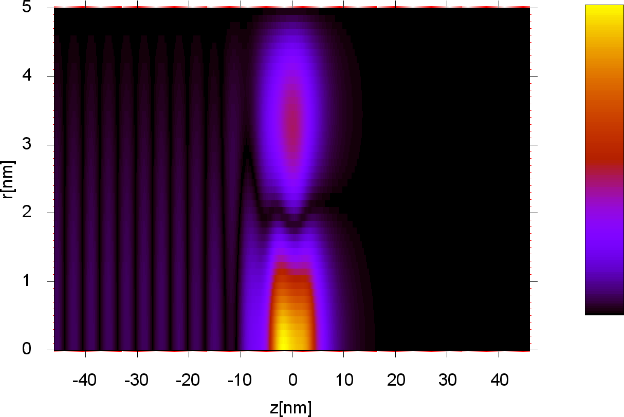
(a) $E=0.217eV$, $n=1$

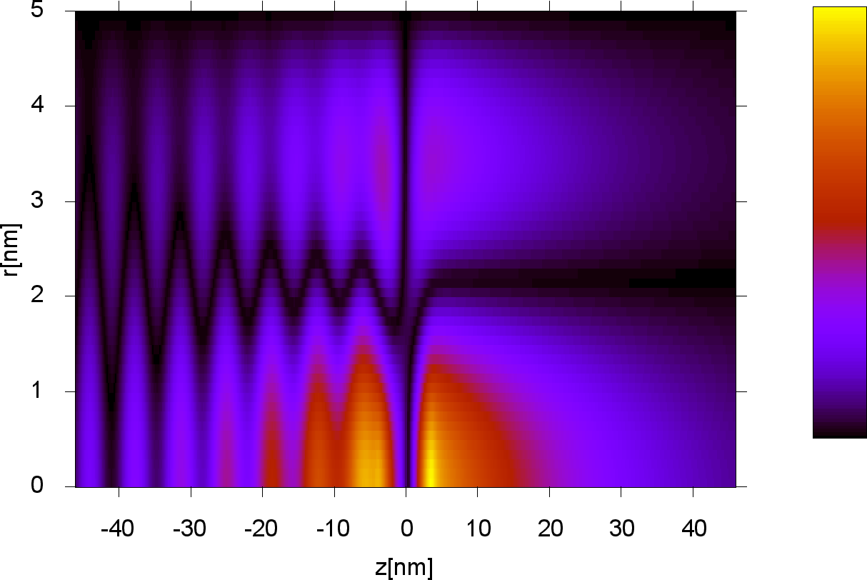
(b) $E=0.243eV$, $n=1$

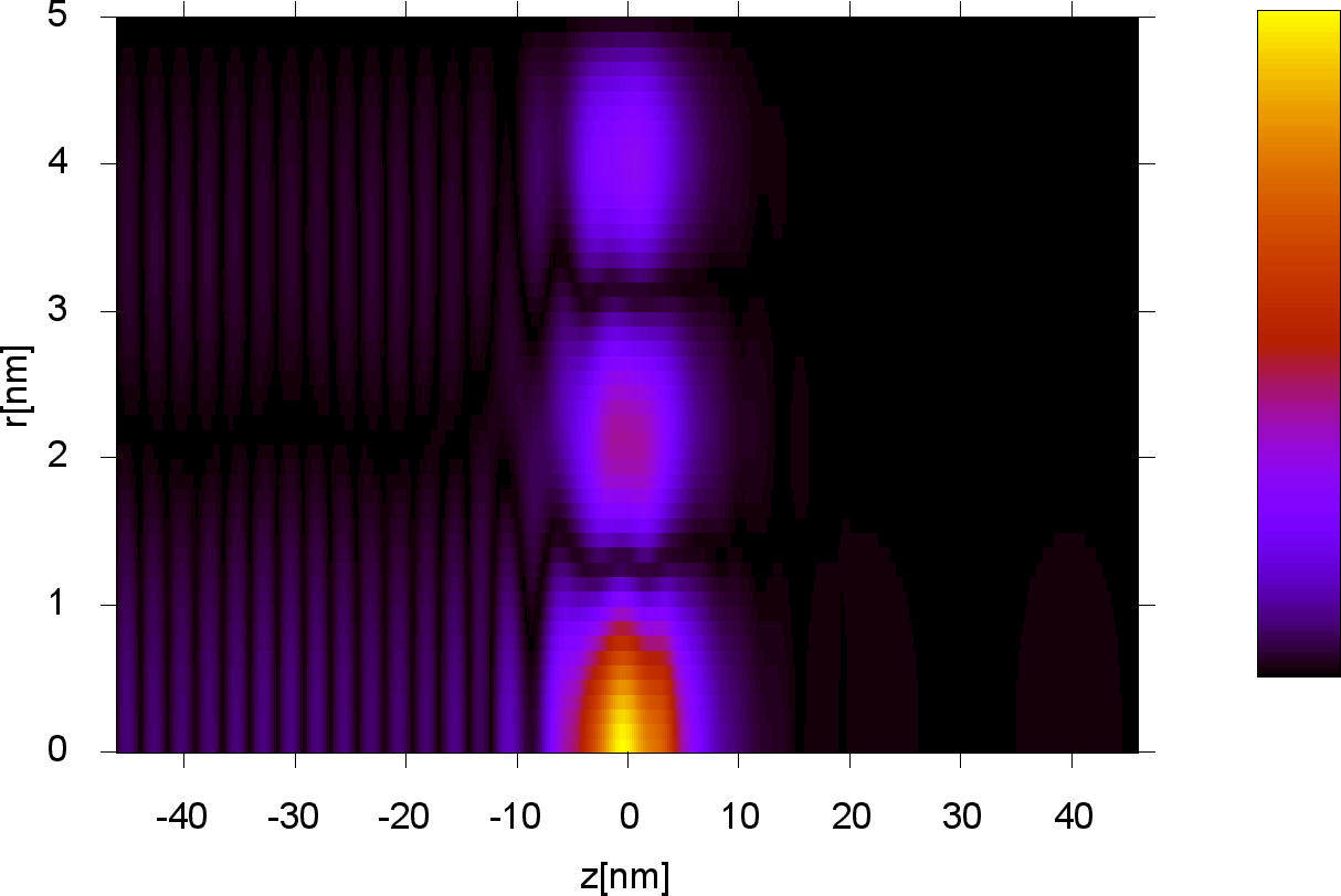
(c) $E=0.576eV$, $n=2$

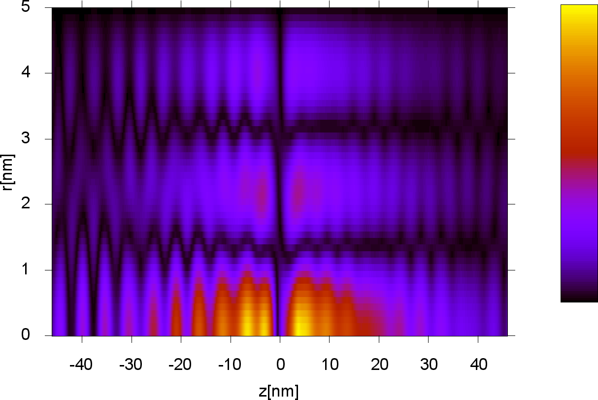
(d) $E=0.600eV$, $n=2$

Figure 10: (color online) Localization probability density $|\psi^{(1)}_{nm}(E,r,z)|^{2}$ for an electron with $m=0$, incident from reservoir $s=1$ into channel $n$ and with energy $E$, both indicated in the captions. The energies correspond to the dips in Fig. 6 for $W_{b}=-0.15eV$.

Increasing the strength of the attractive potential to $W_{b}=-0.15eV$ one can see more dipsBardarson et al. (2004) in the tunneling coefficient in Fig. 6. Interesting is that there are two dips in the first and second plateau for $m=0$, while for $|m|=1$ there is only one dip in every plateau. This can be easily understood if one thinks at the effective attractive potential $V_{nn}$, Eq. (39), created for every subband $n$. In the case of $m\not=0$, the transversal modes $\phi^{(m)}_{n}(r)$ are zero on the cylinder axis, $r=0$, so that the effective potential for every subband is weakened. To confirm that the dips correspond to higher-order quasi-bound states, we plot in Fig. 10 the probability density of the scattering states at the energies corresponding to the two dips in every plateau for $m=0$. For the dips on the first plateau, Figs. 10(a) and 10(b), both scattering wave functions have a node in $r$-direction corresponding to the transversal channel $n=2$. For the dips on the second plateau, Figs. 10(c) and 10(d), the wave functions have two nodes in $r$-direction corresponding to the transversal channel $n=3$. But looking in the $z$-direction, the scattering state for the lower energy dip in every plateau is node-less, while the one for higher-energy dip in every plateau has a node at $z=0$, which is evidence of the second quasi-bound states of the next evanescent channel.

III.2 Core/shell quantum ring

Now, consider the same rectangular quantum well but off-centered. This would corespond to a quantum ring embedded into the nanocylinder, as sketched in Fig. 11 and could be realised in a core-shell heterostructure with suplimentar structuring along the nanowire.

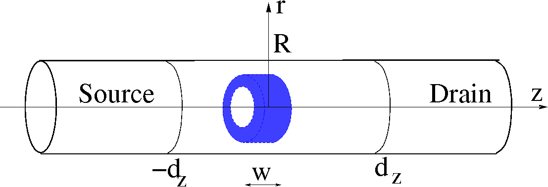
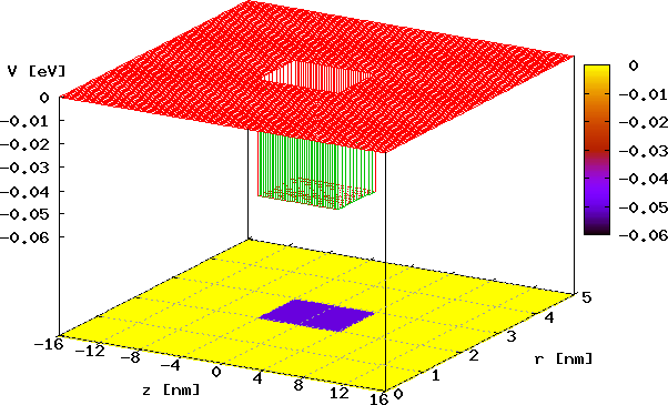
Figure 11: (color onine) a) Sketch of a quantum ring surrounded by the host material. We consider that the ring yields and attractive potential $V(r,z)$ represented in b) by an off-centered rectangular quantum well of depth $W_{b}=-0.05eV$. The thickness of the ring is 1nm, between $R_{1}=2$nm and $R_{2}=3$nm, and the width of the ring is $8$nm. The radius of the cylinder is $R=5$nm.

The tunneling coefficient $T^{(1)}(E)$ for $m=0$ is plotted in Fig. 12, showing the characteristic dips due to the quasi-bound states of the evanescent channels.

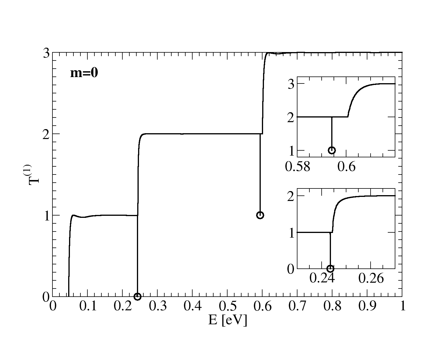
Figure 12: Total tunneling coefficient as function of incident energy $E$ for magnetic quantum numbers $m=0$ for a ring surrounded by the host material. The structure parameters are as in Fig. 11. The symbols show the energies, at which the wave functions are analyzed in the next graphs.

The localization probability density for the energies marked with symbols in Fig. 12 are plotted in Fig. 13.

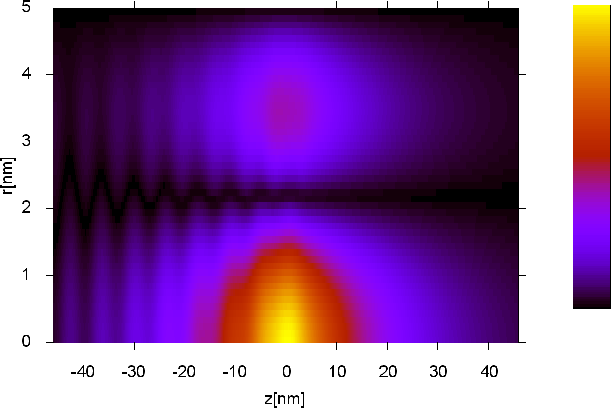
(a) $E=0.243eV$, $n=1$

(b) $E=0.594eV$, $n=2$

Figure 13: (color online) Localization probability density $|\psi^{(1)}_{nm}(E,r,z)|^{2}$ for an electron with $m=0$, incident from reservoir $s=1$ into channel $n$ and with energy $E$ indicated in the captions. The energies correspond to the symbols in Fig. 12.

By shifting the potential from the cylinder axis and keeping the same parameters as for the quantum dot surrounded by the host material, one can recognize the same behavior of the wave functions corresponding to the quasi-bound states as in the previous case. This means that the quasi-bound states of an evanescent channel extend over the whole width of the nanowire, independent where the scattering potential is located in the lateral direction. Similar results hold for $m\not=0$.

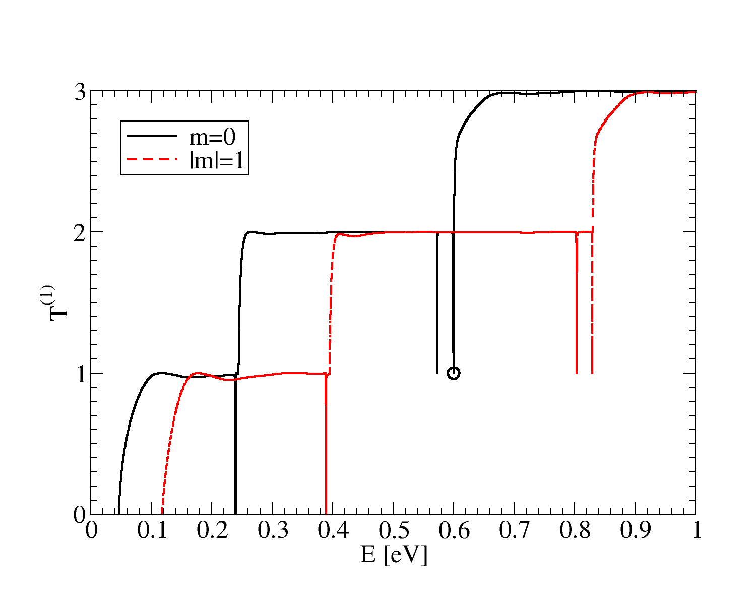
Figure 14: (color online) The tunneling coefficient $T^{(1)}$ for different magnetic quantum numbers $m$ for a ring surrounded by the host material. The parameters are as in Fig. 11, but $W_{b}=-0.15eV$. The symbols show the energies, at which the wave functions are analyzed in the next graphs.

Considering a deeper quantum well one is surprised to see in Fig. 14 that for $m=0$ only one dip appears in the first plateau but two dips in the second plateau. This can be understood considering that if the transversal channels $\phi^{(m)}_{n}(r)$ has a node at the off-centered position of the scattering potential, then $V_{nn}$, Eq. (39), is being weakened allowing for less quasi-bound states.

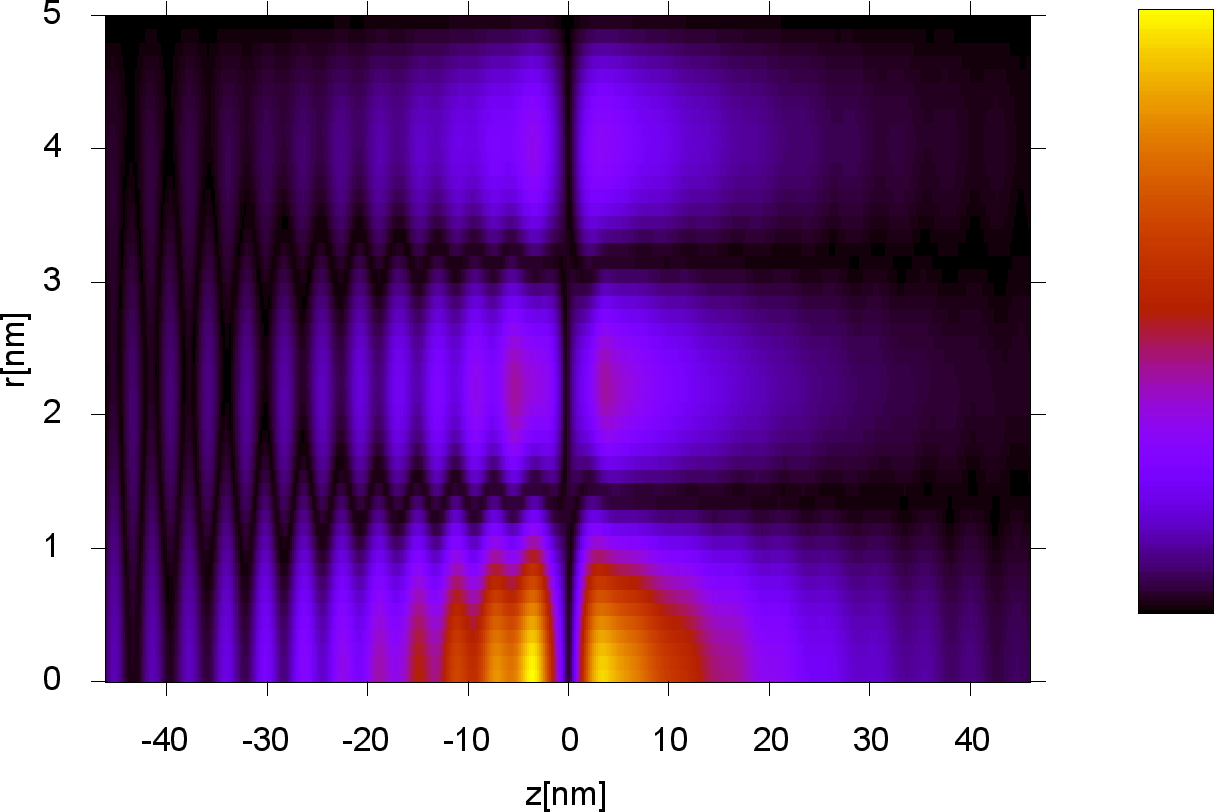
(a) $E=0.599eV$, $n=1$

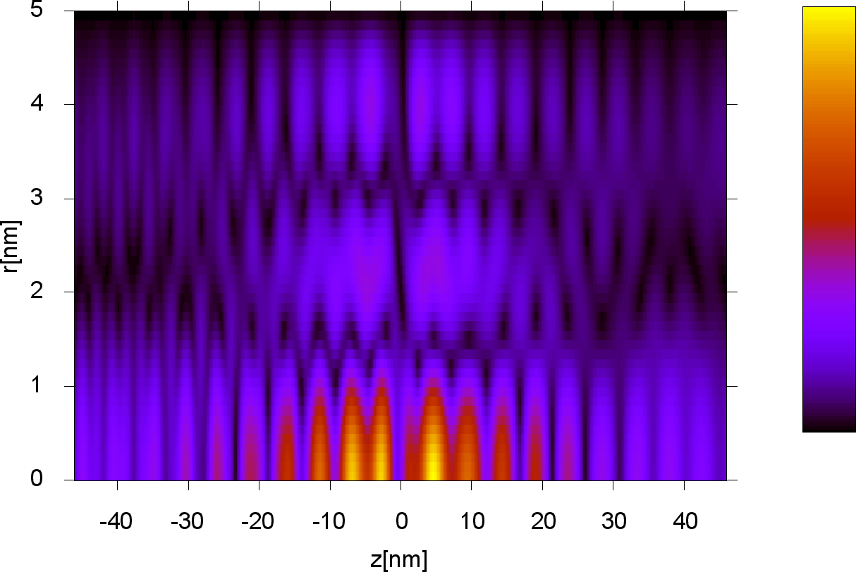
(b) $E=0.599eV$, $n=2$

Figure 15: (color online) Localization probability density $|\psi^{(1)}_{n}(E,r,z)|^{2}$ for an electron with $m=0$, incident from left into both open channels $n=1$ (a) and $n=2$ (b) and with energy $E$ corresponding to the second quasi-bound state on the second plateau in Fig. 14.

Interesting is to take a closer look at the scattering states corresponding to the second quasi-bound state on the second plateau, marked with a symbol in Fig. 14. For this energy, there are two open channels, and we have represented in Fig. 15 the localization probability density for both of them. One can recognize immediately the structure of the wave function with two nodes in $r$-direction corresponding to the third evanescent channel and one node in $z$-direction specific to the second quasi-bound state. Specific for the quasi-bound states of an evanescent channel is also the exponential decaying far from the scattering potential. But the interference patterns on the left and on the right of the scattering potential are quite different for these two scattering wave functions. This can be explained by looking at intrasubband and intersubband transmission probabilities represented in Fig. 16, and which give detailed information about channel mixing.

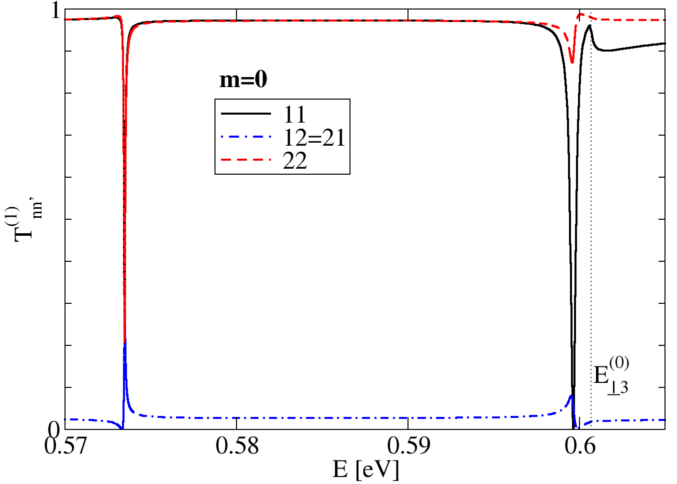
Figure 16: (color online) Intrasubband and intersubband transmission probabilities for a quantum ring (Fig. 11) with $W_{b}=-0.15eV$ and for $m=0$. The curves for $T^{(1)}_{12}$ and $T^{(1)}_{21}$ coincide. The vertical doted line shows the third subband minimum $E^{(0)}_{\perp 3}$.

The intrasubband transmission $T^{(1)}_{11}$ is stronger influenced by channel mixing, showing two pronounced dips, while the intrasubband transmission $T^{(1)}_{22}$ shows only one dip and a second asymmetric Fano line Nöckel and Stone (1994); Racec and Wulf (2001). Both intersubband transmission probabilities $T^{(1)}_{12}$ and $T^{(1)}_{21}$ coincide and show asymmetric Fano lines with zero minima. Now it is clear that there is no interference pattern to the right of the quantum ring in Fig. 15(a) because both transmission probabilities $T^{(1)}_{11}$ and $T^{(1)}_{12}$ are zero for the second quasi-bound state. One recognizes in Fig. 15(a) for the first channel strong interference pattern between the incident part and the reflected part. For the scattering wave function incident on the second channel $T^{(1)}_{22}$ has values close to $1$, and also $T^{(1)}_{21}$ has a maximum. In such a way one sees in Fig. 15(b) right to the scatterer an interference pattern between the transmitted wave in the first channel and the one transmitted in the second channel. One can recognize far from the scattering potential the structure of the second channel with a node in the $r$-direction.

III.3 Double-barrier heterostructure along the nanowire

In Fig. 17 is sketched a double-barrier heterostructure along the cylindrical nanowire. Such systems with sharp interfaces between the layers are realized experimentally based on InAs/InP M.T.Bjork et al. (2002) or on GaAs/AlGaAs Wensorra et al. (2005). We consider rectangular barriers of height $V_{b}=0.5eV$, widths $b=4$nm, and the width of the rectangular quantum well $w=8$nm, as is plotted in Fig. 17.

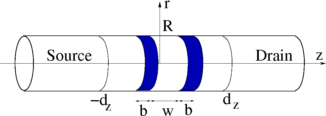
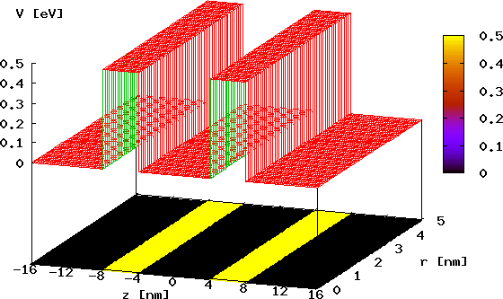
Figure 17: (color online) a) The sketch of a double-barrier heterostructure along the nanowire and b) the scattering potential $V(r,z)$. The height of the barriers is $V_{b}=0.5eV$, the widths of the barriers is $b=4$nm, the width of the quantum well is $w=8$nm and the radius of the nanowire is $R=5$nm.

The total tunneling coefficient $T^{(1)}(E)$ for $m=0$ is plotted in Fig. 18(a) in linear scale. The barriers supprese the transmission, except for a series of sharp peaks due to the quasi-bound states between the barriers. With vertical dashed lines we have represented the energies of the first three transversal channels $E^{(0)}_{\perp,n}$, $n=1,2,3$. One can observe that the tunneling coefficient can reach values higher than 1, if there are more channels open.

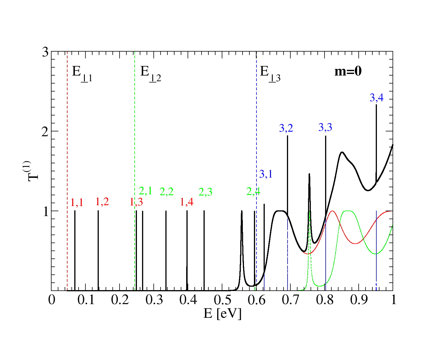
(a) linear scale

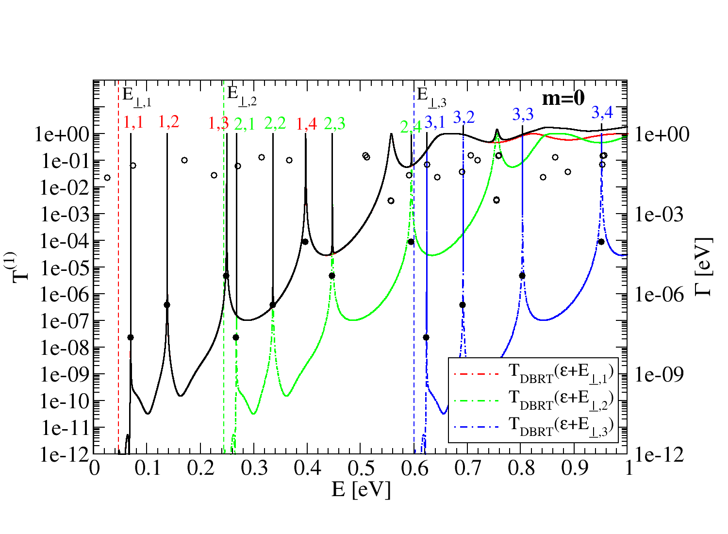
(b) logarithmic scale

Figure 18: (color online) Total tunneling coefficient in linear scale (a) and logarithmic scale (b), as function of incident energy $E$ for a double-barrier heterostructure along the nanowire, as depicted in Fig. 17. The symbols represents the poles: their real part on x-axis and the imaginary part on right y-axis. The peaks are indexed by $(n,i)$, where $n$ denotes the incident channel and $i$ denotes the resonance between the barriers. The same indexes are used in Table 1.

In case of no applied bias between source and drain contact, the scattering potential is separable and has variations only in $z$-direction $V(r,z)=V(z)$, where $V(z)$ describes an 1D double-barrier potential. The scattering does not mix the channels, so that the total tunneling coefficient is given by summation of the intrasubband transmission probabilities for every open channel $T^{(1)}(E)=\sum_{n}T^{(1)}_{nn}(E)$. The intrasubband transmission probability on every open channel is the transmission through a double-barrier structure, but shifted with the transversal energy of the channel $E^{(m)}_{\perp,n}$. So that it can be also computed as for a double-barrier resonant tunneling (DBRT) diode, $T^{(1)}_{nn}(E)=T_{DBRT}(\epsilon+E^{(m)}_{\perp,n})$.

This identity can be used as a verification of the numerical implementation of our method, because the first quantity is computed with the 2D code, while the second quantity is computed with the 1D codeRacec et al. (2002). This is explicitly illustrated in a logarithmic plot of the tunneling coefficient in Fig. 18(b). We represent here by vertical dashed lines the positions of the first three transversal channels $E^{(0)}_{\perp,n}$, $n=1,2,3$. By dot-dashed lines we have represented the tunneling coefficient through the DBRT, but the energies are shifted with the transversal channel energy, as is written in the legend. The curve for the first channel (red dotted line) is just under the total transmission curve (black continuous line). One can observe that the 1D double-barrier potential allows for four resonances (quasi-bound states) between the barriers, i.e. every dashed curve has four peaks below the barrier height.

On the same plot we have plotted with symbols the poles of the current scattering matrix $\tilde{\mathbf{S}}$, computed using the method presented in Ref. [Racec and Wulf, 2001] recently developed for 2D geometries Racec et al. . The real part is on the axis of abscissae, while the imaginary part is on the right axis of ordinates. One can see that among the poles there exist resonant ones, marked by filled symbols, with very low widths, i.e. $\Gamma<10^{-4}eV$, and which are very well separated from the others. Using the same axis of abscissae for the real part and for the tunneling coefficient, one can directly see that to every resonant pole corresponds a transmission peak. Increasing the energy, but keeping the same channel, the widths of the poles increase, and so the widths of the transmission peaks.

This physical interpretation of the tunneling coefficient peaks allows us to label them in Fig. 18 by a pair of numbers $(n,i)$, where $n$ describes the incident channel and $i$ describes the resonance (quasi-bound state) between the barriers.

(n,i)	i=1	i=2	i=3	i=4
n=1
n=2
n=3

Table 1: Localization probability density $|\psi^{(1)}_{n}(E_{res,i},r,z)|^{2}$ for an electron with $m=0$ incident from reservoir $s=1$ into channel $n$ and corresponding to the resonance $i$ between the barriers. The axis of abscissae is $z\in[-8,8]$nm, and the axis of ordinates is $r\in[0,5]$nm for all plots.

In Table 1 are represented the localization probability densities $|\psi^{(1)}_{n}(E_{res,i},r,z)|^{2}$ for the double-barriers region, $z\in[-8,8]$nm and $r\in[0,5]$nm, for every indexed peak in Fig. 18. One can observe that the wave functions have pronounced maxima between the barriers and decrease very quickly inside the barriers. They are localized between the barriers, corresponding, indeed, to resonances (quasi-bound states) between barriers and not to quasi-bound states of evanescent channels. Furthermore, the order $i$ of the resonance between the barriers gives the number of nodes in the $z$-direction, namely $i-1$, while the channel number $n$ gives the number of nodes in the $r$-direction, namely $n-1$. This provides a picture of the orbitals of the ”artificial atom”, which represents this quantum structure Kouwenhoven et al. (2001).

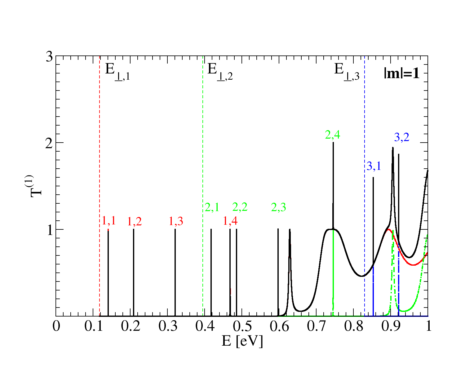
Figure 19: (color online) Transmission coefficient $T^{(1)}$ for $|m|=1$ vs. total energy $E$ for a double-barrier heterostructure along the nanowire as depicted in Fig. 17. The peaks are indexed by $(n,i)$, where $n$ denotes the incident channel and $i$ denotes the resonance between the barriers. The same indexes are used in Table 2.

(n,i)	i=1	i=2	i=3	i=4
n=1
n=2
n=3

Table 2: (color online) Localization probability density $|\psi^{(1)}_{n}(E_{res,i},r,z)|^{2}$ for an electron with $|m|=1$ incident from reservoir $s=1$ into channel $n$ and corresponding to the resonance $i$ between the barriers. The axis of abscissae is $z\in[-8,8]$nm, and the axis of ordinates is $r\in[0,5]$nm for all plots.

Similar behavior is observed for higher magnetic quantum numbers $m$. In Fig. 19 is represented the total tunneling coefficient and in Table 2 the localization probability densities for the indexed peaks for the case $|m|=1$. The positions of the transmission peaks vary for different $m$-values due to the dependence on $m$ of the transversal energy channels $E^{(m)}_{\perp,n}$. The scattering wave functions at resonances for different $m$-values have different positions of nodes in the $r$-direction, and for any $m\not=0$ they are zero on the cylinder axis.

IV Summary and discussion

We have presented a general theory for computing the scattering matrix and the scattering wave functions for a general finite-range extended scattering potential inside a cylindrical nanowire. This formalism was applied to a variety of model systems, like a quantum dot, a quantum ring and a double-barrier heterostructure embedded into the nanocylinder. We have recovered the features for a nonseparable attractive scattering potential in a multi-channel two-probe nanowire taylored in the two-dimensional electron gas. The difference to the Cartesian geometry is that every magnetic quantum number defines a two-dimensional scattering problem with different structure of dips for the same scattering potential. How many of these problems have to be solved depends on the further physical quantity calculation. Furthermore, the cylindrical symmetry does not yield the same ”selection rules” for tunneling coefficient as the Cartesian symmetry, so that dips could be observed in every subband. For stronger attractive potential more than one dip can appear due to the higher-order quasi-bound states of the next evanescent channel. For quasi-bound states localized between barriers, it was possible to compute the poles of the scattering matrix, which provide a quantitative characterization of the resonances. Furthermore, the peaks of resonant tunneling can be indexed by channel number and resonance index. Detailed maps of localization probability density sustain the physical interpretation of the resonances (dips and peaks) found in the studied nanowire heterostructures.

It will be the subject of next works to see, how the buildup of charge around the scattering nonseparable attractive potential influences the overall electrical characteristics of the nanowire-based devices.