On the Solution Space of Differentially Rotating Neutron Stars in General Relativity

Abstract

A highly accurate, multi-domain spectral code is used in order to construct sequences of general relativistic, differentially rotating neutron stars in axisymmetry and stationarity. For bodies with a spheroidal topology and a homogeneous or an $N=1$ polytropic equation of state, we investigate the solution space corresponding to broad ranges of degree of differential rotation and stellar densities. In particular, starting from static and spherical configurations, we analyse the changes of the corresponding surface shapes as the rate of rotation is increased. For a sufficiently weak degree of differential rotation, the sequences terminate at a mass-shedding limit, while for moderate and strong rates of differential rotation, they exhibit a continuous parametric transition to a regime of toroidal fluid bodies. In this article, we concentrate on the appearance of this transition, analyse in detail its occurrence and show its relevance for the calculation of astrophysical sequences. Moreover, we find that the solution space contains various types of spheroidal configurations, which were not considered in previous work, mainly due to numerical limitations.

1 Introduction

Rotating relativistic stars are among the most promising sources of gravitational waves (see Sathyaprakash and Schutz 2009 for a review), especially when they are newly born, be it as proto-neutron stars resulting from a gravitational core collapse or as compact remnants of neutron stars binary mergers. Yet, their study is a complicated task, involving the solution of Einstein’s equations in a dynamical regime while, at the same time, many microphysical phenomena need to be taken into account. Therefore, one of the first compulsory steps in their modelling is the analysis of axisymmetric and stationary configurations of rotating self-gravitating perfect fluids. However, even when a constant rotation profile is assumed, the solution space of this academic problem is known to possess a complex structure (see Ansorg et al. 2004; Meinel et al. 2008), which implies that robust and precise numerical codes are needed before one can proceed with the astrophysical investigation.

A well-studied example is the solution space of homogeneous, uniformly rotating bodies to which, in Newtonian gravity, the famous Maclaurin spheroids belong. For given mass density, this family depends, but for a scaling factor, on only one parameter, for which reason we may refer to it as the Maclaurin sequence. However, the full solution space is much richer as it contains infinitely many Newtonian sequences that branch off from the Maclaurin sequence (see Ansorg et al. 2003b ). Taking these configurations into the realm of general relativity, one recognizes the entire complexity of the solution space which turns out to consist of infinitely many disjoint solution classes (see Ansorg et al. Ansorgetal04 (2004)). Within these classes (which are two-dimensional subsets of the solution space), specific sections of the above Newtonian sequences form particular limiting curves.

One consequence of this class structure is that any continuous sequence of relativistic solutions starting at a static and spherical body and running through the associated spheroidal class, is not connected to the regime of configurations with toroidal shape. Instead, such a sequence eventually leads either to mass shedding limit or to a limit of infinite central pressure.

In a slightly more realistic model of a star, which one obtains by taking polytropic matter, a picture similar to the one depicted above for homogeneous bodies emerges (Meinel et al. Meineletal08 (2008)). As one considers polytropes with increasing polytropic index $N$ (with $N=0$ describing the homogeneous bodies), one finds that the different classes drift apart from one another, implying an even clearer separation between them.

However, apart from the equation of state (EOS), actual stars differ from the model of simple homogeneous rigidly rotating fluids through their presumable differential rotation, which is expected to occur in proto-neutron stars born from a gravitational collapse or from the merger of binary neutron stars. Hence, a natural question that arises is that of the influence of the rotation profile on the main characteristics of a stationary, relativistic star, such as its maximal mass and angular momentum, but also its actual geometrical surface shape. The evolution of the latter one possibly leads to various types of instabilities and corresponding signals (e.g. electromagnetic or gravitational waves, neutrinos). Due to its importance for estimating the delay between a neutron stars binary merger and the collapse to a black hole, this issue was already the topic of various studies, be it for cold or warm equations of state (see Stergioulas S (2003) for a review on rotating stars in relativity). However, in the case of differentially rotating stars, most of the work done up to now seemed to suffer from numerical limitations when the rotation profile started to be too sharp. Moreover, none of those studies really dealt with the changes undergone by the solution space due to the rotation law.

In this article, we focus on the influence of differential rotation on the parameter space of rotating relativistic stars. In particular, we only consider star-like bodies, i.e. configurations with spheroidal topology (simply connected ones), and use two basic EOSs (homogeneous and polytropes with $N=1$) as well as one specific type of rotation law. The latter one is the most classical in general relativity, introduced by Komatsu et al. KEH (1989), in which a parameter $A$ appears that measures the degree by which the rotation is differential. This allows us to go from rigid rotation to configurations with a strong gradient in the rotation profile. As will be described below, in this situation some critical values of $A$ arise, at which a merging of typical classes is exhibited. This result shows that the introduction of several disjoint classes, initially done in order to characterize the solution space corresponding to uniform rotation, only makes sense for sufficiently weak differential rotation.

The paper is organized as follows. First, we clarify the distinction between the so-called spheroidal class and the toroidal class of rotating stars, a notation that should not be confused with the star’s topology, see discussion below. Then, in Section 3, we introduce the Lewis-Papapetrou line element that describes stationary and axisymmetric spacetimes. At the end of that Section we discuss the Komatsu law of differential rotation, to be used in this paper, as well as the resulting general relativistic field equations. In Section 4 we briefly describe particular features of our pseudo-spectral code, used to obtain highly accurate numerical solutions and present numerical results. We introduce four specific types of sequences of differentially rotating relativistic stars, which describe the solution space in question independently of the EOS being chosen. Finally Section 5 provides a summary and a discussion of our results.

2 Spheroidal and toroidal classes

In the following we shall concentrate on two specific classes, which we call spheroidal and toroidal. For rigidly rotating stars, the first one has already been mentioned in the Introduction and contains continuous parametric sequences that start at a static and spherical body. The shapes of these bodies possess spheroidal topology throughout the entire class. Any such sequence eventually leads either to a mass-shedding limit or to a limit of infinite central pressure. For this reason it makes sense to identify extremal values for certain physical quantities, such as the maximal baryon mass, within the spheroidal class.

For the introduction of the toroidal class we consider the so-called Dyson ring sequence, which is the Newtonian sequence of rigidly rotating homogeneous bodies branching off from the Maclaurin sequence at the branch point, at which the Maclaurin spheroids become secularly unstable with respect to the first axisymmetric perturbation (Chandrasekhar chand67 (1967), Bardeen B71 (1971)). One branch of the Dyson ring sequence terminates at a mass-shedding limit, while another one leads to the regime of figures with toroidal topology and finally to arbitrarily thin rings. Taking the Dyson ring solutions into the relativistic regime and choosing again homogeneous matter, we find an associated toroidal class of solutions which is disjoint with respect to the spheroidal class. In contrast to the spheroidal class, it possesses continuous sequences of relativistic solutions leading to infinitely thin tori. Moreover, the solutions of the toroidal class do not possess maximal possible values of the baryon and gravitational masses. Instead, those quantities increase to arbitrarily high values as the relativistic tori become thinner and thinner (see Ansorg et al. 2003c and Fischer et al. Fischeretal05 (2005)).

As explained in the Introduction, the solution space of rigidly rotating $N=1$ polytropes is quite similar, except that even in the Newtonian limit there is already a clear gap between the spheroidal and toroidal sequences. This gap grows further as polytropes with increasing index $N$ are considered.

As an important remark, note that in the above definition of spheroidal and toroidal classes, the existence of continuous transitions, either to spheres or to infinitely thin tori, is considered. This does not determine a priori the geometrical topology of the configurations which form the sequence. This is to say that a body with spheroidal topology (i.e. which is simply connected and has no hole) may in fact belong to the toroidal class, provided that a continuous parameter transition to the regime of infinitely thin tori can be identified.

In this article we focus, for the purpose of simplicity, on stars with spheroidal topology and find that the situation becomes more complicated for differentially rotating bodies. In particular, a merging of the spheroidal and toroidal classes is exhibited, meaning that from some critical rate of differential rotation on the classification does not make sense. However, as we shall see below, a discussion of the corresponding solution space is possible in terms of four different types (A,B,C and D) of one-dimensional parameter sequences.

3 Differentially Rotating Spheroidal Stars in General Relativity

3.1 Line element

Using Lewis-Papapetrou coordinates $(\varrho,z,\varphi,t)$, the line element for a stationary, axially symmetric spacetime corresponding to a rotating perfect fluid configuration can be written in the form (see e.g. Stephani et al. Stephani_etal (2003))

$$\mathrm{d}s^{2}={\rm e}^{2\mu}(\mathrm{d}\varrho^{2}+\mathrm{d}z^{2})+W^{2}{\rm e}^{-2\nu}(\mathrm{d}\varphi-\omega\,\mathrm{d}t)^{2}-{\rm e}^{2\nu}\,\mathrm{d}t^{2},$$ (1)

where the metric functions $\mu$, $W$, $\nu$ and $\omega$ are functions of $\varrho$ and $z$ alone. Note that

$$W=0\qquad\mbox{on the rotation axis $\varrho=0$.}$$ (2)

The coordinates $(\varrho,z,\varphi,t)$ are uniquely defined by the requirement that the metric coefficients and their first derivatives be continuous everywhere, in particular at the surface of the rotating body.

3.2 Equation of state and Rotation law

For a barotropic perfect fluid, the energy-momentum tensor reads

$$T^{ik}=[\epsilon(p)+p]u^{i}u^{k}+pg^{ik}\,,$$ (3)

where $u^{i}$ is the fluid’s 4-velocity. The total mass-energy density $\epsilon$ as a function of the pressure $p$ is given via an equation of state.

In this paper we consider neutron stars described by polytropic or homogeneous EOSs. The polytropic equation of state is given by

$$\epsilon\,(p)=p+\sqrt{p/K}$$ (4)

where $K$ is the polytropic constant. The polytropic index $N$ is chosen to be unity as this value fits well most of the realistic EOSs for neutron stars (see Lattimer & Prakash LattimerP2001 (2006)). Since this is no longer true for strange stars (e.g. Limousin et al. LimousinGG2005 (2005)), whose properties can be much better reproduced using a homogeneous model (see Gondek-Rosińska et al. GondekGH2003 (2003), Amsterdamski et al. Amster2002 (2002)), we also use such an EOS with

$$\epsilon(p)=\epsilon_{0}=\mbox{constant.}$$ (5)

.

The stationary and circular motion of the fluid particles implies a 4-velocity of the form:

$$u^{i}={\rm e}^{-V}(\xi^{i}+\Omega\eta^{i})$$ (6)

where $\xi^{i}$ and $\eta^{i}$ are the Killing vectors with respect to stationarity and axisymmetry respectively. The coefficient $\Omega=u^{t}/u^{\varphi}$ denotes the angular velocity of the fluid and depends on $\varrho$ and $z$. The integrability conditions of the Einstein equations, i.e. the Euler equations

$$T^{ik}_{\;\;\;\;;k}=0$$ (7)

restrict the possible form that the angular velocity can take. They imply

$$-\frac{\mathrm{d}p}{\epsilon+p}=\mathrm{d}V+u^{t}u_{\varphi}\mathrm{d}\Omega$$ (8)

from which it follows that the product $u^{t}u_{\varphi}$ is a function depending on $\Omega$ only,

$$u^{t}u_{\varphi}=F(\Omega),$$ (9)

and that the specific enthalpy

$$h=\frac{\epsilon+p}{\epsilon_{B}}$$ (10)

(where $\epsilon_{B}$ denotes the baryon mass density) with

$$\frac{\mathrm{d}h}{h}=\frac{\mathrm{d}p}{\epsilon+p}$$ (11)

is related to the metric quantities as follows:

$$h=h_{0}\exp\left(V_{0}-V-\int_{\Omega_{c}}^{\Omega}F(\tilde{\Omega})d\tilde{\Omega}\right).$$ (12)

Here, the constant $\Omega_{c}$ denotes the central angular velocity, while $V_{0}$, i.e. the value of the function $V$ at the fluid’s north pole ($\varrho=0,\;z=r_{\mathrm{p}}$), is a relativistic parameter characterizing the rotating fluid body. It is related to the relative redshift $z_{0}$ of photons emitted from the north pole and received at infinity via

$$z_{0}={\rm e}^{-V_{0}}-1.$$

Note that from $u^{i}u_{i}=-1$ we have

$$V=\frac{1}{2}\log\left[{\rm e}^{2\nu}-W^{2}{\rm e}^{-2\nu}(\Omega-\omega)^{2}\right]$$ (13)

and

$$u^{t}u_{\varphi}=\frac{W^{2}(\Omega-\omega)}{{\rm e}^{4\nu}-W^{2}(\Omega-\omega)^{2}}.$$ (14)

Hence, by virtue of (9) we obtain $\Omega$ in terms of the metric coefficients as the solution of the implicit equation

$$F(\Omega)=\frac{W^{2}(\Omega-\omega)}{{\rm e}^{4\nu}-W^{2}(\Omega-\omega)^{2}}.$$ (15)

It follows from (2) and (15) that (i) $F(\Omega_{c})=0$ and (ii) $\Omega=\Omega_{c}$ on the rotation axis.

The enthalpy $h_{0}$ at vanishing pressure takes, for ordinary matter (such as the ones considered here), the value $h_{0}=1$.

The function $F$ can be chosen freely, being only subject to the condition $F(\Omega_{c})=0$. In this paper we use the simplest form which goes beyond uniform rotation, i.e. we take a linear ansatz

$$F(\Omega)\,=\,A^{2}\,(\Omega_{c}\,-\,\Omega)\,,$$ (16)

with the constant $A$ describing the rate of differential rotation. This particular rotation law, originally introduced by Komatsu et al. KEH (1989), has been considered by various authors (including Cook et al. CST (1992), Bonazzola et al. BGSM (1993), Goussard et al. GHZ (1998), Baumgarte et al. Bau00 (2000), Lyford et al. LBS (2003), Morrison et al. MBS (2004), and Villain et al. VPCG (2004)). Since the typical scale of length of the problem is the radius of the star and since the rotation profile becomes uniform in the limit $A\to\infty$, we shall not use $A$ directly, but following Baumgarte et al. Bau00 (2000), we parameterize the sequences and the degree of differential rotation using the parameter

$$\tilde{A}=\hat{A}^{-1}=r_{\mathrm{e}}/A\,,$$ (17)

where $r_{\mathrm{e}}$ is the star’s equatorial coordinate radius. Without entering more into the detail of the law (16) [see Stergioulas S (2003) for further information], we note that it verifies Rayleigh’s criterion for stability against axisymmetric perturbations (Komatsu et al. KEH (1989)) and that, in the Newtonian limit, it reduces to

$$\Omega\,=\,\frac{\Omega_{c}A^{2}}{A^{2}+\varrho^{2}}\,,$$ (18)

which can be shown to be in reasonable agreement with configurations of newly born neutron stars resulting from core collapse (see Section 4 of Villain et al. VPCG (2004)) or from dynamical merger simulations (see Lyford et al. LBS (2003)).

3.3 Einstein equations and the free boundary value problem

The set of equations, following from Einstein’s field equations $R_{ik}-\frac{1}{2}Rg_{ik}=8\pi T_{ik}$ for the metric in the form (1), with (3) and (6), can be written as follows (see e.g. Bardeen & Wagoner BW71 (1971)):

$$\nabla\cdot(B\nabla\nu)-\frac{1}{2}\varrho^{2}B^{3}{\rm e}^{-4\nu}(\nabla\omega)^{2}=$$

$$\hskip 56.9055pt4\pi{\rm e}^{2\mu}B\left[(\epsilon+p)\frac{1+v^{2}}{1-v^{2}}+2p\right],$$ (19a)

$$\nabla\cdot(\varrho^{2}B^{3}{\rm e}^{-4\nu}\nabla\omega)=-16\pi\varrho B^{2}{\rm e}^{2\mu-2\nu}\,(\epsilon+p)\,\frac{v}{1-v^{2}},$$ (19b)

$$\nabla\cdot(\varrho\nabla B)=16\pi\varrho B{\rm e}^{2\mu}p$$ (19c)

$$\mu_{,\varrho\varrho}+\mu_{,\zeta\zeta}-\frac{1}{\varrho}\nu_{,\varrho}+\nabla\nu\left(\nabla\nu-B^{-1}\nabla B\right)=$$

$$\hskip 56.9055pt\frac{1}{4}\varrho^{2}B^{2}{\rm e}^{-4\nu}(\nabla\omega)^{2}-4\pi{\rm e}^{2\mu}(\epsilon+p),$$ (19d)

with [cf. (2)]

$$B:=W/\varrho\quad\text{and}\quad v:=W{\rm e}^{-2\nu}(\Omega-\omega).$$ (19e)

Here the operator $\nabla$ has the same meaning as in a Euclidean three-space in which $\varrho$, $z$ and $\varphi$ are cylindrical coordinates.

The equations (11 - 16) allow us to express $p,\epsilon$ and $\Omega$ and hence all source terms in (19) with respect to the metric potentials and the three constants $\Omega_{c},A$ and $V_{0}$. Thus we obtain a complete set of elliptic equations for the four metric coefficients $\mu$, $B$, $\nu$ and $\omega$.

Note that the fluid’s surface shape is unknown and must be determined in the context of the numerical solution scheme. Its definition is given through vanishing pressure (i.e. through $h=h_{0}$), which leads by virtue of (12) to the surface condition:

$$V=V_{0}-\int_{\Omega_{c}}^{\Omega}F(\tilde{\Omega})d\tilde{\Omega}$$ (20)

The asymptotic conditions at infinity:

$$\mu=\nu=\omega=0,\qquad B=1,$$ (21)

complete the free boundary value problem to be solved. For a given EOS, the corresponding solutions depend on the three parameters $\Omega_{c},A$ and $V_{0}$.

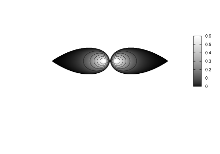
Figure 1: Example of a differentially rotating polytropic body (with polytropic index $N=1$) close to the transition of spheroidal to toroidal topology. The parameters of this configurations are given by $\tilde{A}=0.9,\log h_{\mathrm{max}}=0.6$ and $r_{\mathrm{p}}/r_{\mathrm{e}}=0.005$. In the corresponding diagram in fig. 3 this body belongs to the sequence which terminates in a mass-shedding limit ($\tilde{\beta}=0$) at $r_{\mathrm{p}}/r_{\mathrm{e}}\approx 0.25$. The plot shows isocontours of $\log h$ in a meridional cross section. The strongly pronounced cusp at the equatorial edge indicates that this configuration rotates almost at the mass-shedding limit.

4 Numerical results

4.1 Numerical scheme and parameter prescriptions

We use a pseudo-spectral double-domain method to compute highly accurate numerical solutions corresponding to rotating relativistic stars. This technique has been described in detail in Ansorg et al. Ansorgetal02 (2002); 2003a , see also Meinel et al. Meineletal08 (2008). Here we develop the scheme further to include the calculation of differentially rotating stars. In particular, strongly pinched objects can be computed (for an example see fig. 1).

As a special feature, the code permits the prescription of three independent parameters which may be chosen for convenience. For example, it is possible to prescribe the parameter triple $(h_{\mathrm{max}},r_{\mathrm{p}}/r_{\mathrm{e}},\tilde{A})$ where $h_{\mathrm{max}}$ denotes the maximal enthalpy of the star. Note that this maximal value need not be assumed in the coordinate origin $\varrho=z=0$ but can, for stars sufficiently close to the toroidal regime, be located at $(\varrho_{h},z=0)$ with $\varrho_{h}>0$, see e.g. fig. 1. The dotted line on each diagram of figures 3 and 5 separates configurations with the maximal enthalpy located in the stellar center (on the right side) from those having $h_{\mathrm{max}}$ outside the coordinate origin. This curve is defined by the vanishing of the enthalpy’s second derivative with respect to $\varrho$ at the origin, i.e. through $(\mathrm{d}^{2}h/\mathrm{d}\varrho^{2})_{c}=0$. We determine such a configuration through the prescription of the triples $(h_{\mathrm{max}},r_{\mathrm{p}}/r_{\mathrm{e}},(\mathrm{d}^{2}h/\mathrm{d}\varrho^{2})_{c})$ or $(h_{\mathrm{max}},\tilde{A},(\mathrm{d}^{2}h/\mathrm{d}\varrho^{2})_{c})$.

Another possible parameter prescription is the triple $(h_{\mathrm{max}},r_{\mathrm{p}}/r_{\mathrm{e}},\beta)$ where the shedding parameter $\beta$ is defined as in Ansorg et al. 2003a ,

$$\beta=\left.-\frac{r_{\mathrm{e}}^{2}}{r_{\mathrm{p}}^{2}}\;\frac{\mathrm{d}(z_{b}^{2})}{\mathrm{d}(\varrho^{2})}\right|_{\varrho=r_{\mathrm{e}}}$$ (22)

with $z=z_{b}(\varrho)$ describing the star’s surface. This parameter is chosen such that $\beta=0$ in the mass-shedding limit and $\beta=1$ for (Maclaurin) spheroids. If a sequence exhibits the transition to the toroidal regime (i.e. $r_{\mathrm{p}}/r_{\mathrm{e}}\to 0$), $\beta$ tends to infinity as this transition is encountered. For this reason we prefer to consider the rescaled shedding parameter

$$\tilde{\beta}=\frac{\beta}{1+\beta}$$ (23)

which tends to 0 in the mass-shedding limit, to $\frac{1}{2}$ for the Maclaurin spheroids as well as in the spherical non-rotating limit and to 1 at the transition point to the toroidal regime.

For the exact calculation of the critical rotation law parameter $\tilde{A}_{\mathrm{crit}}$, marking the onset of a continuous parametric transition of non-rotating spherical stars to toroidal configurations, the parameter triple $(h_{\mathrm{max}},r_{\mathrm{p}}/r_{\mathrm{e}},\tilde{\beta})$ proves to be particularly useful. At fixed value $h_{\mathrm{max}}$, the parameter $\tilde{A}$ can be interpreted as a function of the two variables $r_{\mathrm{p}}/r_{\mathrm{e}}$ and $\tilde{\beta}$. As will be discussed below, this function possesses a saddle point with the value $\tilde{A}=\tilde{A}_{\mathrm{crit}}$. Hence it can be found by solving the equations

$$\left(\frac{\partial\tilde{A}}{\partial(r_{\mathrm{p}}/r_{\mathrm{e}})}\right)_{h_{\mathrm{max}}}=0=\left(\frac{\partial\tilde{A}}{\partial\tilde{\beta}}\right)_{h_{\mathrm{max}}}$$ (24)

for the corresponding parameters $(r_{\mathrm{p}}/r_{\mathrm{e}})_{\mathrm{crit}}$ and $\tilde{\beta}_{\mathrm{crit}}$. The associated $\tilde{A}$ assumed for the parameter triple $(h_{\mathrm{max}},(r_{\mathrm{p}}/r_{\mathrm{e}})_{\mathrm{crit}},\tilde{\beta}_{\mathrm{crit}})$ is the critical value $\tilde{A}_{\mathrm{crit}}$ in question. In order to determine $\tilde{A}_{\mathrm{crit}}$ accurately, we compute the function $\tilde{A}=\tilde{A}(r_{\mathrm{p}}/r_{\mathrm{e}},\tilde{\beta})$ in a vicinity of the critical point and perform a numerical differentiation with respect to the two variables. We then solve the system (24) by means of a Newton-Raphson scheme. Note that again a pseudo-spectral treatment ensures a high accuracy of the value $\tilde{A}_{\mathrm{crit}}$ obtained in this manner.

4.2 Polytropic bodies

Figure 2: Type A-, B-, C- and D-sequences of differentially rotating polytropic fluid bodies (polytropic index $N=1$) with prescribed maximal enthalpy $\log h_{\mathrm{max}}=0.2$. Shown is the dependency between the shed parameter $\tilde{\beta}$ and the ratio $r_{\mathrm{p}}/r_{\mathrm{e}}$ of polar to equatorial coordinate radius for several values of the rotation law parameter $\tilde{A}$. The bold curve corresponds to the separatrix sequence with $\tilde{A}=\tilde{A}_{\mathrm{crit}}=0.75904$.

In order to illustrate the evolution of the solution space as the rate $\tilde{A}$ of differential rotation is increased, we consider at first fairly weak relativistic polytropic solutions (with polytropic index $N=1$) with a fixed maximal enthalpy, $\log h_{\mathrm{max}}=0.2$.

For rigid rotation, i.e. $\tilde{A}=0$, the sequence starting from static and spherical bodies with $r_{\mathrm{p}}/r_{\mathrm{e}}=1$ runs through the spheroidal class and terminates in a mass-shedding limit characterized by $\tilde{\beta}=0$, see fig. 2. We assign type A to sequences of this kind and note that the spheroidal class is made up of such sequences.

Associated with the sequence of type A with $\tilde{A}=0$, there is a sequence that contains only configurations with toroidal shape and belongs to the toroidal class. It runs within class II in figure 3.29 of Meinel et al. Meineletal08 (2008) from the mass-shed curve to the extreme Kerr limit. Since in fig. 2 only sequences with spheroidal topology (i.e. $r_{\mathrm{p}}>0$) are displayed, this sequence does not appear here.

However, as we move to $\tilde{A}=0.4$ we now find this sequence in the left part of the figure. It is clearly separated from the corresponding sequence of type A which runs through the spheroidal class (in the right part of the figure). This means that, for $\tilde{A}=0.4$, the sequence belonging to the toroidal class stretches into the regime of bodies with spheroidal topology, i.e. the toroidal class contains configurations with spheroidal topology. We assign type B to sequences of this kind, that appear for $\tilde{A}$ greater than some threshold value to be studied in a forthcoming article. In the corresponding situation for $\tilde{A}=0.7$, the two sequences of types A and B still coexist, but they have moved towards one another. The merging of the two sequences appears at the critical value $\tilde{A}_{\mathrm{crit}}=0.75904$. The further increase of $\tilde{A}$ leads again to two separate sequences of types C and D. The type C sequences show a continuous transition from the regime of spherical (with $r_{\mathrm{p}}/r_{\mathrm{e}}=1$) to that of toroidal bodies (at $r_{\mathrm{p}}/r_{\mathrm{e}}=0$). The type D sequences possess mass-shedding limits (with $\tilde{\beta}=0$) at both ends. As these two ends tend towards one another as $\tilde{A}$ is increased, this type of sequence exists only for a small range of values of the parameter $\tilde{A}$. This range has the lower bound $\tilde{A}_{\mathrm{crit}}$ and another threshold value as an upper bound (to be studied elsewhere). At this upper bound the sequence of type D degenerates to a single point describing a particular mass-shedding fluid body. By contrast, the type C sequences exist for all values $\tilde{A}>\tilde{A}_{\mathrm{crit}}$.

The qualitative behaviour for $\log h_{\mathrm{max}}=0.2$ is typical for the entire solution space. In fig. 3 we show sequences for $\tilde{A}\in\{0,0.1,0.2,\ldots,1.5\}$ and $\log h_{\mathrm{max}}\in\{0,0.2,0.4,0.6\}$, $\log h_{\mathrm{max}}=0$ meaning the Newtonian limit. The lowermost curves on the right part of the diagrams always correspond to rigid rotation $\tilde{A}=0$, while the uppermost ones represent the configurations with the highest rotation parameter considered, $\tilde{A}=1.5$. Also shown (in bold) are the separation sequences corresponding to the values $\tilde{A}_{\mathrm{crit}}$. From fig. 2 it becomes apparent that at the separation point the function $\tilde{A}=\tilde{A}(r_{\mathrm{p}}/r_{\mathrm{e}},\tilde{\beta})$ has a maximum with respect to the variable $r_{\mathrm{p}}/r_{\mathrm{e}}$ and a minimum with respect to the variable $\tilde{\beta}$, i.e. a saddle point at which (24) holds. Moreover the curves described by $(\mathrm{d}^{2}h/\mathrm{d}\varrho^{2})_{c}=0$ are plot (dotted lines), which indicate that, for configurations to the left of this curve, the maximal enthalpy is assumed outside the coordinate origin.

Note that for $\log h_{\mathrm{max}}=0.6$ two branches of the separatrix sequence (for which $\tilde{A}_{\mathrm{crit}}=0.77804$) run into the regime of toroidal figures, as opposed to only one such branch for $\log h_{\mathrm{max}}\in\{0,0.2,0.4\}$. As a consequence, the neighbouring sequences with shedding ends (i.e. in the diagram for $\log h_{\mathrm{max}}=0.6$, type D curves with $\tilde{A}=0.8$ and $\tilde{A}=0.9$) possess a branch running into the toroidal regime. However, the type D sequence for $\tilde{A}=1$ is still solely formed of figures with spheroidal topology.

The evolution of the parameter $\tilde{A}_{\mathrm{crit}}$ as a function of $\log h_{\mathrm{max}}$ is displayed in fig. 4. From this figure it can be seen that for a sufficiently large rate of differential rotation, $\tilde{A}>\tilde{A}^{\mathrm{N=1}}_{\mathrm{min}}=0.71085$, the spheroidal and toroidal classes merge and hence a continuous parametric transition of spherical to toroidal differentially rotating stars is exhibited. The merging of the classes occurs for $\tilde{A}=\tilde{A}^{\mathrm{N=1}}_{\mathrm{min}}$ at $\log h_{\mathrm{max}}=0.3845$.

4.3 Homogeneous bodies

Figure 3: Sequences of differentially rotating polytropic fluid bodies (polytropic index $N=1$) with prescribed maximal enthalpies $\log h_{\mathrm{max}}$ for $\tilde{A}\in\{0,0.1,0.2,\ldots,1.5\}$. Uppermost and lowermost curves on the right part of the diagrams correspond to rotation parameters $\tilde{A}=1.5$ and $\tilde{A}=0$ (rigid rotation) respectively. The solid bold curves represent the separatrix sequences with $\tilde{A}=\tilde{A}_{\mathrm{crit}}$, and the dotted curves defined by $(\mathrm{d}^{2}h/\mathrm{d}\varrho^{2})_{c}=0$ indicate that, for configurations to the left of these curves, the maximal enthalpy is assumed outside the coordinate origin. Note that the diagram for $\log h_{\mathrm{max}}=0$ displays Newtonian sequences.

For homogeneous and rigidly rotating fluid bodies in General Relativity, the Newtonian limiting sequences have been found to be the separatrix sequences that separate the general-relativistic solution classes from one another, see Ansorg et al. Ansorgetal04 (2004), figs 4 and 5 therein. Specifically, the Maclaurin spheroids with $r_{\mathrm{p}}/r_{\mathrm{e}}\in[0.17126,1]$ form one branch of the separatrix dividing the spheroidal from the toroidal class. Other branches of this particular separatrix are formed by the Maclaurin spheroids with $r_{\mathrm{p}}/r_{\mathrm{e}}\in[0.11160,0.17126]$ and the (non-relativistic) Dyson ring sequence (marked by $A_{1}^{\pm}$ in fig. 4 of Ansorg et al. Ansorgetal04 (2004)).

In the diagram for $\log h_{\mathrm{max}}=0$, fig. 5, we find the same sequences to be the branches of the separatrix which divides particular sequences of differentially rotating Newtonian bodies from one another. We mark this separatrix by a bold curve. The Maclaurin spheroids are characterized by $\tilde{\beta}=\frac{1}{2}$, and the two branches discussed above can easily be identified. The Dyson ring sequence leads from a mass-shedding end $\tilde{\beta}=0$ across the Maclaurin sequence to the regime of toroidal bodies (at $r_{\mathrm{p}}/r_{\mathrm{e}}=0$). The remaining piece of the separatrix is given by the sequence $A_{2}^{+}$ in fig. 4 of Ansorg et al. 2003b and leads also from the mass-shedding limit $\tilde{\beta}=0$ to the Maclaurin sequence.

The separatrix composed of these segments looks qualitatively similar to its polytropic counterpart in fig. 3. For differential rotation $\tilde{A}>0$ we find sequences of type C in the upper right and of type D in the lower left part of the panel, but neither type A nor type B. Note that the only type D curve displayed ‘inside’ the lower separatrix branches corresponds to $\tilde{A}=0.1$, just as the type C curve located opposite and next to the separation crossing point $(r_{\mathrm{p}}/r_{\mathrm{e}}=0.17126,\tilde{\beta}=\frac{1}{2})$.

The curves printed in chain lines belong to the Maclaurin sequence with $r_{\mathrm{p}}/r_{\mathrm{e}}<0.11160,\tilde{\beta}=\frac{1}{2}$ as well as to the sequence $A_{2}^{-}$ in fig. 4 of Ansorg et al. 2003b , i.e. to branches of separatrices dividing ‘higher’ solution classes from one another.

In the remaining diagrams of fig. 5 we display sequences for $\tilde{A}\in\{0,0.1,0.2,\ldots,1.5\}$ and $\log h_{\mathrm{max}}\in\{0.2,0.4,0.6\}$. As in fig. 3, the lowermost curves on the right part of the diagrams always correspond to rigid rotation $\tilde{A}=0$, while the uppermost ones represent the configurations with the highest rotation parameter considered, $\tilde{A}=1.5$. Again, bold lines describe the separatrix sequences, and the dotted lines in all diagrams of fig. 5 are sequences with $(\mathrm{d}^{2}h/\mathrm{d}\varrho^{2})_{c}=0$.

For a given value $\log h_{\mathrm{max}}$ the qualitative picture for homogeneous bodies is similar to that for polytropes, i. e. we can identify sequences of types A and B for $\tilde{A}<\tilde{A}_{\mathrm{crit}}$ and those of types C and D for $\tilde{A}>\tilde{A}_{\mathrm{crit}}$. However, the onset of the spheroidal-toroidal transition as a function of $\log h_{\mathrm{max}}$ is very different, see fig. 6. If one restricts oneself to differential rotation parameters $\tilde{A}<\tilde{A}^{\mathrm{N=1}}_{\mathrm{min}}$, then any sequence of polytropic bodies starting at the spherical limit $r_{\mathrm{p}}/r_{\mathrm{e}}=1$ ends in a mass-shedding limit $\tilde{\beta}=0$ with some value $r_{\mathrm{p}}/r_{\mathrm{e}}>0$ (and consequently is of type A). This means that in this range of differential rotation we have a clear gap between the spheroidal and the toroidal class. The distinction between the classes only disappears for $\tilde{A}>\tilde{A}^{\mathrm{N=1}}_{\mathrm{min}}$ in which case all four types of sequences can be found. In contrast, the solution space of differentially rotating homogeneous bodies with $\tilde{A}>0$ does not allow at all a classification with respect to spheroidal and toroidal classes. All four types of sequences can be identified in the small range $0<\tilde{A}<\tilde{A}^{\mathrm{hom}}_{\mathrm{max}}=0.29646$, and for $\tilde{A}>\tilde{A}^{\mathrm{hom}}_{\mathrm{max}}$ we find only type C and D sequences. That is to say that then any sequence starting at the spherical limit $r_{\mathrm{p}}/r_{\mathrm{e}}=1$ leads to the transition to the toroidal regime (and hence is of type C).

Figure 4: For polytropic bodies (polytropic index $N=1$), the critical rotation parameter $\tilde{A}_{\mathrm{crit}}$ is plot against the maximal enthalpy, $\log h_{\mathrm{max}}$. For parameters below this curve, each sequence starting at the spherical and static limit terminates at a mass-shedding limit $\tilde{\beta}=0$. On the other hand, such sequences lead to the transition to the toroidal regime if the parameters chosen are located above the curve.

Figure 5: Sequences of differentially rotating homogeneous fluid bodies with prescribed maximal enthalpies $\log h_{\mathrm{max}}$ for $\tilde{A}\in\{0,0.1,0.2,\ldots,1.5\}$. Uppermost and lowermost curves on the right part of the diagrams correspond to rotation parameters $\tilde{A}=1.5$ and $\tilde{A}=0$ (rigid rotation) respectively. As in fig. 3, the solid bold curves represent the separatrix sequences with $\tilde{A}=\tilde{A}_{\mathrm{crit}}$ and the dotted curves are defined by $(\mathrm{d}^{2}h/\mathrm{d}\varrho^{2})_{c}=0$. Note that the diagram for $\log h_{\mathrm{max}}=0$ displays Newtonian sequences, some of which divide ’higher’ solution classes from one another. See the text for more detail.

Figure 6: For homogeneous bodies, the critical rotation parameter $\tilde{A}_{\mathrm{crit}}$ is plot against the maximal enthalpy, $\log h_{\mathrm{max}}$. As in fig. 4, parameters below or above this curve describe sequences starting at the spherical and static limit and leading to a mass-shedding limit or to the toroidal regime respectively.

5 Summary and discussion

In this paper, we have constructed relativistic models of differentially rotating neutron stars with spheroidal topology (no hole) for broad ranges of degree of differential rotation $\tilde{A}\in\{0,0.1,0.2,\ldots,1.5\}$ and for maximal enthalpies $\log h_{\mathrm{max}}\in\{0,0.2,0.4,0.6\}$. We have considered homogeneous and polytropic configurations (with polytropic index $N=1$) and adopted the rotation law introduced by Komatsu et al. KEH (1989).

From the results obtained we may conclude that the structure of disjoint classes in the solution space of relativistic configurations is a special feature of the sub-space corresponding to rigid rotation. It turned out that this concept does not survive in the entire solution space of differentially rotating stars. Instead we find that from a critical rate of differential rotation on, a classification cannot be introduced. For differential rotation larger than this critical rate, the previously disjoint classes have merged and we find continuous transitions from non-rotating and spherical to toroidal objects.

The critical rotation rate depends strongly on the equation of state being chosen. While the space of sufficiently weakly differentially rotating polytropes still permits the class structure in question, there is no non-vanishing rate of differential rotation for which such a classification makes sense in the case of homogeneous bodies.

We have described properties of the general structure of the solution space in terms of four types of one-dimensional parameter sequences:

• Sequences of type A exist for $\tilde{A}<\tilde{A}_{\mathrm{crit}}$ and consist solely of spheroidal configurations. These sequences start at a static and spherical body and end at the mass shedding limit. Most of these configurations have the maximum enthalpy located in the stellar center, but not all of them (for exceptions see e.g. fig. 3, panel for $\log h_{\mathrm{max}}=0.6$, type A sequences in the vicinity of the separatrix curve).

• Sequences of type B also exist for $\tilde{A}<\tilde{A}_{\mathrm{crit}}$. They start at the mass shedding limit and have a continuous parametric transition to a regime of bodies with toroidal topology. The branch with spheroidal topology configurations exists only for $\tilde{A}$ larger than a threshold value.

• Sequences of type C exist for $\tilde{A}>\tilde{A}_{\mathrm{crit}}$. They start at a static and spherical body and possess a transition to arbitrarily thin rings. Consequently, type C sequences contain configurations with spheroidal and toroidal topology.

• Sequences of type D also exist for $\tilde{A}>\tilde{A}_{\mathrm{crit}}$, but only in a narrow range of values of $\tilde{A}$. Their two extremities are configurations at the mass shedding limit.

In the solution space, the type A- and B-sequences are clearly separated from the type C- and D-sequences by specific separatrix curves which we determined in a rigorous numerical procedure. These separatrix curves, emphasized through bold solid lines in the figures 2, 3 and 5, have in most cases considered three branches that end in the regime of spheroidal bodies and one branch that leads to toroidal bodies. Note that in fig. 3, in the diagram for $\log h_{\mathrm{max}}=0.6$, an exception can be seen, namely two branches leading to toroidal topology.

The fact that the classification in classes fails in the realm of differentially rotating bodies means that a new interpretation of the criterion of the maximal mass for the distinction between a black hole and a rotating neutron star (see e.g. reasoning in Baumgarte et al. Bau00 (2000)) becomes necessary. While Baumgarte et al. Bau00 (2000) discussed an increase of the maximum mass of differentially rotating stars, we find here that the family of sufficiently strongly differentially rotating bodies does not possess a maximum at all for the stars’ (baryon and gravitational) masses. Evidently, one can always define one maximal value, restricting the calculation to simply connected bodies, as we did in this study, but that is not physically relevant since as the full family contains arbitrarily thin toroidal figures, the mass values may become arbitrarily large (see Ansorg et al. 2003c and Fischer et al. Fischeretal05 (2005)). In a forthcoming article, we shall come back to this mass criterion and its application to differentially rotating fluids.

In this article the complexity of the full solution space of differentially rotating fluid bodies was demonstrated, which could only be revealed by means of a precise and flexible code that can provide predictions which are relevant from the astrophysical point of view. Indeed, it should be noticed that the critical values obtained for $\tilde{A}$ ($\sim 0.7$) are associated with a degree of differential rotation that is quite similar to what was obtained in dynamical simulations of merging binary neutron stars based on such EOSs (see Shibata & Uryu SU (2000)). This means that for the study of properties of stationary configurations, considered as mimics of a specific phase before the collapse to a black hole, the existence of multiple possible configurations has to be kept in mind during the numerical calculations, in order to determine properly an actual sequence and not one built from configurations belonging to different types.

References

- (1) Amsterdamski, P., Bulik, T., Gondek-Rosińska, D., Kluźniak, W.,2002 ,A&A, 381, L21
- (2) Ansorg, M., Kleinwächter, A., & Meinel, M., 2002, A&A, 381, L49
- (3) Ansorg, M., Kleinwächter, A., & Meinel, R. 2003a, A&A, 405, 711
- (4) Ansorg, M., Kleinwächter, A. ,& Meinel, R. 2003b, MNRAS, 339, 515
- (5) Ansorg, M., Kleinwächter, A., & Meinel, R. 2003c, ApJ, 582, L87
- (6) Ansorg, M., Fischer, T., Kleinwächter, A., Meinel, M., Petroff, D., & Schöbel, K. 2004, MNRAS, 335, 682
- (7) Bardeen, J.M. 1971, ApJ, 167, 425
- (8) Bardeen, J.M. & Wagoner, R. V. 1971, ApJ, 167, 359
- (9) Baumgarte, T.W., Shapiro, S.L., & Shibata, M. 2000, ApJ, 528, L29
- (10) Bonazzola, S., Gourgoulhon, E., Salgado M., & Marck J.-A. 1993, A&A 278, 421
- (11) Chandrasekhar, S. 1967, ApJ, 147, 334
- (12) Cook, G.B., Shapiro, S.L., & Teukolsky, S.A. 1992, ApJ, 398, 203
- (13) Fischer, T., Horatschek, S. & Ansorg, M. 2005, MNRAS, 364, 943
- (14) Gondek-Rosińska, D., Gourgoulhon, E., Haensel, P.,2003, A&A, 412, 777
- (15) Gourgoulhon, E., Haensel, P., Livine, R., Paluch, E., Bonazzola, S., & Marck, J.-A. 1999, A&A, 349, 851
- (16) Goussard, J.O., Haensel, P., & Zdunik, J.L. 1998, A&A, 330, 1005
- (17) Komatsu, H., Eriguchi, Y., & Hachisu, I. 1989, MNRAS, 237, 355
- (18) Lattimer, J.M., Prakash, M. 2006, ApJ, 550, 426
- (19) Limousin, F., Gondek-Rosińska, D., Gourgoulhon, E., 2005, Phys. Rev. D, 71, 064012
- (20) Lorimer, D.R., ”Binary and Millisecond Pulsars”, Living Rev. Relativity 8, (2005), 7. URL (cited on September 2007): http://www.livingreviews.org/lrr-2005-7
- (21) Lyford, N. D., Baumgarte, T. W., & Shapiro, S. L. 2003, ApJ, 583, 410
- (22) Meinel, R., Ansorg, M., Kleinwächter, A., Neugebauer, G. & Petroff, D. 2008 , Relativistic Figures of Equilibrium, Cambridge University Press, New York
- (23) Morrison, I.A., Baumgarte, T.W., & Shapiro, S.L. 2004, ApJ, 610, 941
- (24) Piran, T. 2005, Rev. Mod. Phys., 76, 1143
- (25) Sathyaprakash, B.S., Schutz, B.F., ”Physics, Astrophysics and Cosmology with Gravitational Waves”, Living Rev. Relativity 12, (2009), 2. URL (cited on 2009/03/10): http://www.livingreviews.org/lrr-2009-2
- (26) Shibata, M., Uryu, K. 2000, Phys. Rev. D, 61, 064001
- (27) Stephani, H., Kramer, D., MacCallum, M. A. H., Hoenselaers, C., & Herlt, E. 2003, Exact Solutions of Einstein’s Field Equations, Cambridge University Press
- (28) Stergioulas, N. 2003, Living Rev. Relativity 6, URL (cited on 07-2007): http://www.livingreviews.org/lrr-2003-3
- (29) Villain, L., Pons, J.A., Cerda-Duran, P., & Gourgoulhon, E. 2004, A&A, 418, 283