Possible treatment of the Ghost states in the Lee-Wick Standard Model

Abstract

Very recently, the Lee-Wick standard model has been introduced as a non-SUSY extension of the Standard model which solves the Hierarchy problem. In this model, each field kinetic term attains a higher derivative term. Like any Lee-Wick theory, this model suffers from existence of Ghost states. In this work, we consider a prototype scalar field theory with its kinetic term has a higher derivative term, which mimics the scalar sector in the Lee-Wick Standard model. We introduced an imaginary auxiliary field to have an equivalent non-Hermitian two-field scalar field theory. We were able to calculate the positive definite metric operator $\eta$ in quantum mechanical and quantum field versions of the theory in a closed form. While the Hamiltonian is non-Hermitian in a Hilbert space with the Dirac sense inner product, it is Hermitian in a Hilbert space endowed by the inner product $\langle n|\eta|m\rangle$ as well as having a correct-sign propagator (no Lee-Wick fields). Besides, the obtained metric operator also diagonalizes the Hamiltonian in the two fields ( no mixing). Moreover, the Hermiticity of $\eta$ constrained the two Higgs masses to be related as $M>2m$, which has been obtained in another work using a very different regime and thus supports our calculation. Also, an equivalent Hermitian (in the Dirac sense) Hamiltonian is obtained which has no Ghost states at all, which is a forward step to make the Lee-Wick theories more popular among the Physicists.

One of the greatest puzzles in Particle Physics is the Hierarchy problem DJOUADI . SUSY was invented to solve this problem susy . However, very recently and on the guidance of a previous work of Lee and Wick lee1 ; lee2 , a Lee-Wick (LW) extension of the standard model has been introduced and investigated lee-wick ; caron ; LHD ; neutrino . While the LW QED is a finite theory, the non-Abealian LW gauge theory is not finite. Although it is not finite, it has been shown that it solves the Hierarchy problem too.

The main idea of any Lee-Wick model is that the regulator in Pauli-Villars corresponds to a physical degree of freedom. However, a  QED with a Photon propagator with the regulator term is a theory with higher derivative. A great puzzle that makes such trends in the theory of particle physics not popular is that they include exotic fields called the Lee-Wick fields. For instance, in the LW extension of standard model every field of the conventional standard model has a higher derivative kinetic term and it has been shown that the theory can be converted into an equivalent one with more fields but some of them has a propagator with wrong sign (exotic).

In a very different kind of studies, Carl Bender and Philip D Mannheim have shown that a quantum mechanical theory with higher derivatives which apparently suffers from negative norm problem can be converted into an equivalent one with the ghost states are disappeared noghost . In showing that, they stressed a higher derivative Pais-Uhlenbeck model. In fact, the regime of $\mathcal{PT}$ -symmetric theories has been used successfully in some other works abophi41p1 ; abophi61p1 ; bendr . In this letter, we show that the ideas can successfully applied to the different sectors in the LW Standard model introduced very recently. For that, we shall stress a type of scalar field theory very similar to that employed in the Lee-Wick standard model. We show that the theory is free from ghost states which then leads to the enhancement of the popularity of the Lee-Wick standard model as a possible theory free from ghosts as well as does not suffer from the Hierarchy puzzle.

A prototype scalar field Lagrangian introduced in the Lee-Wick standard model is lee-wick ;

$$\mathcal{L}=\frac{1}{2}\partial_{\mu}\phi\partial^{\mu}\phi-\frac{1}{2M^{2}}\left(\partial^{2}\phi\right)^{2}-\frac{1}{2}m^{2}\phi^{2}.$$ (1)

Fellowing the work in Ref. lee-wick , one can introduce an auxiliary field $\phi_{2}$ to get rid of the higher derivative in the theory such that;

$$\mathcal{L}=\frac{1}{2}\partial_{\mu}\phi\partial^{\mu}\phi-\frac{1}{2}m^{2}\phi^{2}-\phi_{2}\partial^{2}\phi+\frac{1}{2}M^{2}\phi_{2}^{2},$$ (2)

From the equation of motion of $\phi_{2}$ we get;

$$\frac{\partial\mathcal{L}}{\partial\left(\partial_{\mu}\phi_{2}\right)}=0,\text{ \ \ \ \ \ }\frac{\partial\mathcal{L}}{\partial\phi_{2}}=\phi_{2}M^{2}-\partial^{2}\phi.\text{\ }$$

Then, the auxiliary field $\phi_{2}$ is given by the relation

$$\phi_{2}=\frac{1}{M^{2}}\partial^{2}\phi.$$

Let us define

$$\phi=\phi_{1}-\phi_{2},$$

Then;

$$\mathcal{L} =\frac{1}{2}\partial_{\mu}\left(\phi_{1}-\phi_{2}\right)\partial^{\mu}\left(\phi_{1}-\phi_{2}\right)-\frac{1}{2}m^{2}\left(\phi_{1}-\phi_{2}\right)^{2}-\phi_{2}\partial^{2}\left(\phi_{1}-\phi_{2}\right)+\frac{1}{2}M^{2}\phi_{2}^{2},$$

$$=\frac{1}{2}\partial_{\mu}\phi_{1}\partial^{\mu}\phi_{1}+\frac{1}{2}\partial_{\mu}\phi_{2}\partial^{\mu}\phi_{2}-\partial_{\mu}\phi_{2}\partial^{\mu}\phi_{1}-\phi_{2}\partial^{2}\phi_{1}+\phi_{2}\partial^{2}\phi_{2}$$ (3)

$$-\frac{1}{2}m^{2}\left(\phi_{1}-\phi_{2}\right)^{2}+\frac{1}{2}M^{2}\phi_{2}^{2},$$

$$=\frac{1}{2}\partial_{\mu}\phi_{1}\partial^{\mu}\phi_{1}-\frac{1}{2}\partial_{\mu}\phi_{2}\partial^{\mu}\phi_{2}-\frac{1}{2}m^{2}\phi_{1}^{2}+\frac{1}{2}\left(M^{2}-m^{2}\right)\phi_{2}^{2}\allowbreak+m^{2}\phi_{2}\phi_{1}.$$

The Hamiltonian corresponding to the Lagrangian in Eq.(3) can be obtained as;

$$H=\frac{\pi_{1}^{2}}{2}+\frac{1}{2}\left(\nabla\phi_{1}\right)^{2}+\frac{1}{2}m^{2}\phi_{1}^{2}-\frac{\pi_{2}^{2}}{2}-\frac{1}{2}\left(\nabla\phi_{2}\right)^{2}-\frac{1}{2}\left(M^{2}-m^{2}\right)\phi_{2}^{2}-m^{2}\phi_{1}\phi_{2}$$ (4)

Now, let us apply the canonical transformation $\phi_{2}\rightarrow i\phi_{2},\pi_{2}\rightarrow-i\pi_{2}$ which preserve the commutation relation noghost ;

$$\left[\phi_{2}\left(x\right),\pi_{2}\left(y\right)\right]=\left[i\phi_{2}\left(x\right),-i\pi_{2}\left(y\right)\right]=i\delta^{3}\left(x-y\right).$$ (5)

Then the transformed Hamiltonian will take the form;

$$H=\frac{\pi_{1}^{2}}{2}+\frac{1}{2}\left(\nabla\phi_{1}\right)^{2}+\frac{1}{2}m^{2}\phi_{1}^{2}+\frac{\pi_{2}^{2}}{2}+\frac{1}{2}\left(\nabla\phi_{2}\right)^{2}+\frac{1}{2}\left(M^{2}-m^{2}\right)\phi_{2}^{2}-im^{2}\phi_{1}\phi_{2}$$ (6)

In other words, the negative norm manifested in the work of Ref.lee-wick by a negative kinetic term of the LW field ($\phi_{2}$) is manifested here by the non-Hermiticity of the theory represented by the Lagrangian in Eq. (3). By assuming that $\phi_{2}$ is a pseudo scalar, the Hamiltonian obtained from Eq. (3) is $\mathcal{PT}$-symmetric too. Indeed, non-Hermitian $\mathcal{PT}$-symmetric theories are suffering from the existence of ghost states however there exists known algorithms to recover such problemsspect ; spect ; noghost . In fact, though the Hamiltonian in Eq.(6) is non-Hermitian in the Dirac sense, it is not only Hermitian in a Hilbert space endowed by the inner product $\langle n|\eta|m\rangle$ spect ; spect1 , where $\eta$ is a positive definite metric operator, but also the kinetic terms have the correct form.

To start the algorithm of curing the ghost states problem in the theory, for simplicity, let us investigate, first, the theory in $0+1$ dimensions (Quantum mechanics). Since the Hamiltonian in Eq.(6) is pseudo-Hermitian, one can seek a positive definite metric operator of the form;

$$\eta=\exp\left(2\left(\omega_{1}\pi_{1}\phi_{2}+\omega_{2}\pi_{2}\phi_{1}\right)\right),$$

where $\omega_{1}$ and $\omega_{2}$ are two real parameters to be obtained later in terms of the mass parameters $m$ and $M$. Note that $\eta$ is Hermitian and has the property spect ; spect1

$$\eta H\eta^{-1}=H^{\dagger}.$$ (7)

Also, $\rho=\sqrt{\eta}$ has the property

$$\rho H\rho^{-1}=h,$$ (8)

where $h$ is a Hermitian (in the Dirac sense) as well as positive normed Hamiltonian equivalent to $H$.

To determine the parameters $\omega_{1}$ and $\omega_{2}$, we consider the transformations of the different fields in the Hamiltonian under the effect of $\rho$ as follows;

$$\rho\phi_{1}\rho^{-1} =\phi_{1}-i\omega_{1}\phi_{2},$$

$$\rho\pi_{1}\rho^{-1} =\pi_{1}+i\omega_{2}\pi_{2},$$

$$\rho\phi_{2}\rho^{-1} =\phi_{2}-i\omega_{2}\phi_{1},$$

$$\rho\pi_{2}\rho^{-1} =\pi_{2}+i\omega_{1}\pi_{1}.$$

Accordingly;

$$h =\frac{\left(\pi_{1}+i\omega_{2}\pi_{2}\right)^{2}}{2}+\frac{1}{2}m^{2}\left(\phi_{1}-i\omega_{1}\phi_{2}\right)^{2}+\frac{\left(\pi_{2}+i\omega_{1}\pi_{1}\right)^{2}}{2}$$

$$+\frac{1}{2}\left(M^{2}-m^{2}\right)\left(\phi_{2}-i\omega_{2}\phi_{1}\right)^{2}-im^{2}\left(\phi_{1}-i\omega_{1}\phi_{2}\right)\left(\phi_{2}-i\omega_{2}\phi_{1}\right),$$

or

$$h =\frac{1}{2}\pi_{1}^{2}+i\pi_{1}\omega_{2}\pi_{2}-\frac{1}{2}\omega_{2}^{2}\pi_{2}^{2}+\frac{1}{2}m^{2}\phi_{1}^{2}-\frac{1}{2}m^{2}\omega_{1}^{2}\phi_{2}^{2}+\frac{1}{2}\pi_{2}^{2}+i\pi_{2}\omega_{1}\pi_{1}$$

$$-\frac{1}{2}\omega_{1}^{2}\pi_{1}^{2}\frac{1}{2}\left(M^{2}-m^{2}\right)\left(\phi_{2}^{2}-\omega_{2}^{2}\phi_{1}^{2}\right)-m^{2}\omega_{2}\phi_{1}^{2}-m^{2}\omega_{1}\phi_{2}^{2}-im^{2}\phi_{1}\phi_{2}$$ (9)

$$+im^{2}\omega_{1}\allowbreak\phi_{2}\omega_{2}\phi_{1}-i\phi_{2}\omega_{2}\phi_{1}M^{2}+i\phi_{2}\omega_{2}\phi_{1}m^{2}-im^{2}\phi_{1}\omega_{1}\phi_{2}.$$

For $h$ to be Hermitian, one has to put the constraints

$$i\omega_{2}+i\omega_{1} =0,$$

$$\left(-m^{2}+m^{2}\omega_{1}\omega_{2}-\omega_{2}M^{2}+\omega_{2}m^{2}-m^{2}\omega_{1}\right) =0,$$ (10)

on the introduced parameters $\omega_{1}$ and $\omega_{2}$. Equivalently, we have the relations

$$\omega_{1} =-\omega_{2},$$

$$-m^{2}-m^{2}\omega_{1}^{2}+\omega_{1}M^{2}-2m^{2}\omega_{1} =0.$$ (11)

In terms of the mass parameters, $\omega_{1}$ can be obtained as

$$\omega_{1}=\frac{1}{2m^{2}}\left(M^{2}-2m^{2}\pm\sqrt{M^{4}-4M^{2}m^{2}}\right).$$ (12)

Also, due to the reality of $\omega_{1}$, the two Higgs masses are related by;

$$M^{2}\geqslant 4m^{2},$$

which agrees with the results in Ref.lee-wick

Then the Hermitian Hamiltonian $h$ has the form;

$$h =\frac{1}{2}\pi_{1}^{2}\left(1-\omega_{1}^{2}\right)+\frac{1}{2}m^{2}\phi_{1}^{2}+\frac{1}{2}\left(1-\omega_{1}^{2}\right)\pi_{2}^{2}-\frac{1}{2}m^{2}\omega_{1}^{2}\phi_{2}^{2}$$

$$+\frac{1}{2}\left(M^{2}-m^{2}\right)\left(\phi_{2}^{2}-\omega_{1}^{2}\phi_{1}^{2}\right)+m^{2}\omega_{1}\phi_{1}^{2}-m^{2}\omega_{1}\phi_{2}^{2},$$

$$=\frac{1}{2}\pi_{1}^{2}\left(1-\omega_{1}^{2}\right)+\frac{1}{2}m^{2}\phi_{1}^{2}+\frac{1}{2}\left(1-\omega_{1}^{2}\right)\pi_{2}^{2}$$

$$+\left(\frac{1}{2}m^{2}\omega_{1}^{2}+m^{2}\omega_{1}-\frac{1}{2}M^{2}\omega_{1}^{2}\right)\phi_{1}^{2}$$

$$+\left(-\frac{1}{2}m^{2}\omega_{1}^{2}+\frac{1}{2}M^{2}-m^{2}\omega_{1}-\frac{1}{2}m^{2}\right)\phi_{2}^{2}.$$

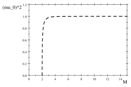
Figure 1: The factor $\mu_{0}^{2}=(1-\omega^{2})$ plotted against the mass parameter $M$ for $m=1$. One can realize that the factor is positive for the available range of $M$.

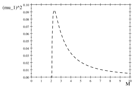
Figure 2: A contribution to the mass parameter squared of the field $\phi_{1}$ of the form $\mu_{1}^{2}=\left(\frac{1}{2}m^{2}\omega_{1}^{2}+m^{2}\omega_{1}-\frac{1}{2}M^{2}\omega_{1}^{2}\right)$ in the Hermitian Hamiltonian $h$, plotted against the mass parameter $M$ for $m=1$. Since the other contribution is $m^{2}$ and from the plot $\mu_{1}^{2}$ is always positive the mass squared as a whole is positive.

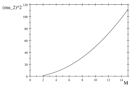
Figure 3: The mass parameter squared of the field $\phi_{2}$ given by $\mu_{2}^{2}=-\frac{1}{2}m^{2}\omega_{1}^{2}+\frac{1}{2}M^{2}-m^{2}\omega_{1}-\frac{1}{2}m^{2}$ in the Hermitian Hamiltonian $h$, plotted against the mass parameter $M$ for $m=1$, which is again a positive quantity.

To make sure that the negative norm problem has been lifted, we plotted the propagator-sign governing factors of the form $\mu_{0}^{2}=\left(1-\omega_{1}^{2}\right)$, $\ \mu_{1}^{2}=\left(\frac{1}{2}m^{2}\omega_{1}^{2}+m^{2}\omega_{1}-\frac{1}{2}M^{2}\omega_{1}^{2}\right)$ and $\mu_{2}^{2}=\left(-\frac{1}{2}m^{2}\omega_{1}^{2}+\frac{1}{2}M^{2}-m^{2}\omega_{1}-\frac{1}{2}m^{2}\right)$ as a function of $M$ for $m=1$,  in Fig.1., Fig.2. and Fig.3, respectively. In these plots, we have taken the root $\omega_{1}=\frac{1}{2m^{2}}\left(M^{2}-2m^{2}-\sqrt{M^{4}-4M^{2}m^{2}}\right)$, while the other root represents a theory of indefinite norm. One can realize that all these factors are positive for the available range of $M$ which assures the remedy of the wrong sign in the propagator of the LW field.

In higher dimensions (Quantum field theory), one needs to deal with operator densities and thus the metric operator will take the from;

$$\eta=\int d^{3}z\exp\left(2\left(\omega_{1}\pi_{1}\left(z\right)\phi_{2}\left(z\right)+\omega_{2}\pi_{2}\left(z\right)\phi_{1}\left(z\right)\right)\right).$$

Accordingly, we have the relations

$$\rho\phi_{1}\left(x\right)\rho^{-1} =\phi_{1}\left(x\right)-i\omega_{1}\int d^{3}z\phi_{2}\left(z\right)\delta^{3}(x-z),$$

$$\rho\pi_{1}\rho^{-1} =\pi_{1}+i\omega_{2}\int d^{3}z\pi_{2}\left(z\right)\delta^{3}(x-z),$$

$$\rho\phi_{2}^{-1}\rho^{-1} =\phi_{2}-i\omega_{2}\int d^{3}z\phi_{1}\left(z\right)\delta^{3}(x-z),$$

$$\rho\pi_{2}^{-1}\rho^{-1} =\pi_{2}+i\omega_{1}\int d^{3}z\pi_{1}\left(z\right)\delta^{3}(x-z).$$

And thus

$$\rho\phi_{1}^{-1}\rho^{-1} =\phi_{1}-i\omega_{1}\phi_{2},$$

$$\rho\pi_{1}^{-1}\rho^{-1} =\pi_{1}+i\omega_{2}\pi_{2},$$

$$\rho\phi_{2}^{-1}\rho^{-1} =\phi_{2}-i\omega_{2}\phi_{1},$$

$$\rho\pi_{2}^{-1}\rho^{-1} =\pi_{2}+i\omega_{1}\pi_{1}.$$

Also, note that

$$\rho\frac{1}{2}\left(\nabla\phi_{1}(x)\right)^{2}\rho^{-1} =\frac{1}{2}\left(\nabla\phi_{1}(x)\right)^{2}-i\omega_{1}\nabla_{x}\phi_{1}(x)\nabla_{x}\phi_{2}(x)-\frac{\omega_{1}^{2}}{2}\left(\nabla_{x}\phi_{2}(x)\right)^{2},$$

$$\rho\frac{1}{2}\left(\nabla\phi_{2}(x)\right)^{2}\rho^{-1} =\frac{1}{2}\left(\nabla\phi_{2}(x)\right)^{2}-i\omega_{2}\nabla_{x}\phi_{1}(x)\nabla_{x}\phi_{2}(x)-\frac{\omega_{2}^{2}}{2}\left(\nabla_{x}\phi_{1}(x)\right)^{2}.$$ (13)

Again, with the choice $\omega_{1}=-\omega_{2}=\omega$, one gets;

$$\rho\left(\frac{1}{2}\left(\nabla\phi_{1}(x)\right)^{2}+\frac{1}{2}\left(\nabla\phi_{2}(x)\right)^{2}\right)\rho^{-1}=\frac{1}{2}\left(1-\omega^{2}\right)\left(\nabla\phi_{1}(x)\right)^{2}+\left(\nabla\phi_{2}(x)\right)^{2},$$ (14)

and the quantum field Hermitian Hamiltonian takes the form;

$$h =\frac{1}{2}\pi_{1}^{2}\left(1-\omega^{2}\right)+\frac{1}{2}\left(1-\omega^{2}\right)\left(\nabla\phi_{1}(x)\right)^{2}+\frac{1}{2}m^{2}\phi_{1}^{2}$$

$$+\frac{1}{2}\left(1-\omega^{2}\right)\pi_{2}^{2}+\frac{1}{2}\left(1-\omega^{2}\right)\left(\nabla\phi_{2}(x)\right)^{2}+\frac{1}{2}M^{2}\phi_{2}^{2}$$

$$+\left(\frac{1}{2}m^{2}\omega^{2}+m^{2}\omega-\frac{1}{2}M^{2}\omega_{1}^{2}\right)\phi_{1}^{2}$$ (15)

$$+\left(-\frac{1}{2}m^{2}\omega_{1}^{2}-m^{2}\omega_{1}-\frac{1}{2}m^{2}\right)\phi_{2}^{2}.$$

One can easily realize that the governing factors are all positive for the available range of the mass parameter $M$ relative to the mass parameter $m$. Accordingly, the problem of wrong sign propagator has been recovered. Another benefit of the transformation mapping $H\rightarrow h$, is that there exists no mixing terms in $h$ ($h$ is diagonal in the fields $\phi_{1}$ and $\phi_{2}$) .

To make sure that the Hermitian equivalent Hamiltonian in Eq.(15) still bears the feature of quadratic divergence cancellation we rewrite it in the form;

$$h =h_{1}+h_{2},$$

$$h_{1} =\frac{1}{2}\left(\pi_{1}^{2}+\left(\nabla\phi_{1}\right)^{2}\right)+\frac{1}{2}m^{2}\left(1+\omega_{1}\right)^{2}\phi_{1}^{2}$$

$$+\frac{1}{2}\left(-\omega_{1}^{2}\right)\left(\pi_{2}^{2}+\left(\nabla\phi_{2}\right)^{2}\right)+\frac{1}{2}\left(-m^{2}\left(1+\omega_{1}\right)^{2}\right)\phi_{2}^{2},$$

$$h_{2} =\frac{1}{2}\left(\pi_{2}^{2}+\left(\nabla\phi_{2}\right)^{2}\right)+\frac{1}{2}M^{2}\phi_{2}^{2}+\frac{1}{2}\left(-\omega_{1}^{2}\right)\left(\pi_{1}^{2}+\left(\nabla\phi_{1}\right)^{2}\right)$$

$$+\frac{1}{2}\left(-M^{2}\omega_{1}^{2}\right)\phi_{1}^{2},$$

which shows that although $h$ is Hermitian and positive normed it can be decomposed into two terms each of which has the from of a normal and a Lee-Wick fields.

Conclusions

We considered a higher derivative scalar field theory of the form used in the Lee-Wick standard model. We were able to obtain a non-Hermitian but $\mathcal{PT}$-symmetric two-field equivalent Hamiltonian. Using the tools applied to pseudo Hermitian Hamiltonians, we were able to obtain the positive definite metric operator both on the quantum mechanical and quantum field versions of the theory in a closed form. The so obtained equivalent Hermitian Hamiltonian has propagators of correct sign which mean that the Ghost problem has been cured. Moreover, the Hermitian Hamiltonian is diagonal in the fields. Note that, we discarded the potential term as it is used to break the symmetry and has no effect of the negative norm of the auxiliary field and thus one can add it at the end to the equivalent Hermitian Hamiltonian we obtained. We assert that the work presented here is fully new as it is the first time to obtain the exact metric operator for a realistic quantum field theory. Also, the idea here can be applied to all the sectors in the Lee-wick standard model and thus obtain a theory which is non-SUSY, has no Ghosts, as well as solves the Hierarchy problem. A note to be mentioned is that the mass of the auxiliary field is greater than the normal Higgs which means that it is out of any experimental tests carried out. We aim that in proving the non-existence of Ghosts in a Lee-Wick theory we make those theories attract the attentions of researchers as they introduce finite Quantum Electrodynamics theory as well as showing up a standard model free from the Hierarchy problem.

References

• (1) Abdelhak DJOUADI, The Anatomy of Electro–Weak Symmetry Breaking, arXiv:hep-ph/0503172.
• (2) J. Wess and B. Zumino, Nucl. Phys. B 70 (1974) 39.
• (3) T. D. Lee and G. C. Wick, Nucl. Phys. B 9, 209 (1969).
• (4) T. D. Lee and G. C. Wick, Phys. Rev. D 2, 1033 (1970).
• (5) BenjamΓ­n Grinstein, Donal O’Connell, and Mark B. Wise, Phys.Rev.D77:025012 (2008).
• (6) C.Β D.Β Carone and R.Β F.Β Lebed, Phys.Β Lett.Β B 668, 221 (2008).
• (7) Thomas G. Rizzo, JHEP0706:070 (2007).
• (8) JosΓ© RamΓ³n Espinosa, BenjamΓ­n Grinstein, Donal O’Connell
and Mark B. Wise, Phys.Rev.D77:085002 (2008).
• (9) Carl M. Bender and Philip D. Mannheim, Phys.Rev.Lett.100:110402(2008).
• (10) Carl Bender and Stefan Boettcher, Phys.Rev.Lett.80:5243-5246 (1998).
• (11) Abouzeid shalaby, Phys.Rev.D76:041702 (2007 ).
• (12) Abouzeid shalaby, Eur.Phys.J.C50:999-1006 (2007).
• (13) A. Mostafazadeh, J. Math. Phys., 43, 3944 (2002).
• (14) A. Mostafazadeh, J. Math. Phys. 43, 205 (2002).
Refer to caption