Unusual features of coarsening with detachment rates decreasing with cluster mass

Abstract

We study conserved one-dimensional models of particle diffusion, attachment and detachment from clusters, where the detachment rates decrease with increasing cluster size as $\gamma(m)\sim m^{-k}$, $k>0$. Heuristic scaling arguments based on random walk properties show that the typical cluster size scales as ${\left(t/\ln{t}\right)}^{z}$, with $z=1/\left(k+2\right)$. The coarsening of neighboring clusters is characterized by initial symmetric flux of particles between them followed by an effectively assymmetric flux due to the unbalanced detachement rates, which leads to the above logarithmic corrections. Small clusters have densities of order $t^{-mz\left(1\right)}$, with $z\left(1\right)=k/\left(k+2\right)$. Thus, for $k<1$, the small clusters (mass of order unity) are statistically dominant and the average cluster size does not scale as the size of typically large clusters does. We also solve the Master equation of the model under an independent interval approximation, which yields cluster distributions and exponent relations and gives the correct dominant coarsening exponent after suitable changes to incorporate effects of correlations. The coarsening of typical large clusters is described by the distribution $P_{t}\left(m\right)\sim 1/t^{y}f\left(m/t^{z}\right)$, with $y=2z$. All results are confirmed by simulation, which also illustrates the unusual features of cluster size distributions, with a power law decay for small masses and a negatively skewed peak in the scaling region. The detachment rates considered here can apply in the presence of strong attractive interactions, and recent applications suggest that even more rapid rate decays are also physically realistic.

I Introduction

Domain growth in far from equilibrium conditions is observed in phase separation of mixtures, dynamics of glasses and island coarsening during or after deposition of a thin film, among other systems bray94 ; ritort ; mevansreview ; robin . This motivated the proposal of many statistical models which exhibit growth laws for the typical domain size in the form $l\sim t^{z}$, where $z$ is a coarsening exponent mevansreview . For instance, when a system is quenched from an homogeneous phase into a broken-symmetry phase, two universality classes are frequently found, one of them of curvature driven (or diffusive) growth allen ; ohta , with $z=1/2$, and the other of conserved scalar order parameter slyozov ; huse , with $z=1/3$. However, many model dynamics do not obey detailed balance and may lead to domain growth with other power law forms or with anomalous coarsening, in which with $l$ grows slower than any power of time. A continuous range of coarsening exponents may be obtained by tuning a single parameter in models with relatively simple physical mechanisms, e. g. single particle exchange between clusters bennaim ; igloi . On the other hand, anomalous coarsening is found in certain models that mimic glassy behavior or phase separation east ; kafri (such behaviour is also present in models with detailed balance under certain conditions shore ). A range of coarsening behaviors is also obtained experimentally, e. g. in recent works on shaken granular systems (${\left(\log{t}\right)}^{1/2}$) granular , separation of mixtures of milk protein and amylopectin ($0.04\leq z\leq 0.2$) bont and air bubbles in foams ($0.2\leq z\leq 0.5$) schmitt . Despite the variety of possible scenarios which were already shown in the literature, the study of simple models with normal or anomalous coarsening is still important because it may reveal the basic microscopic mechanisms that lead to certain macroscopic behavior. Such basic studies may also help the development of more realistic models for a wide range of processes, such as those in Ref. mccoy .

A class of models in which islands grow via particle diffusion, attachment and detachment (Ostwald ripening) is very important in surface science because they can explain many features of submonolayer or multilayer growth cv ; biehl ; etb . Even the one-dimensional models are important in this field, both as a first step to understand realistic two-dimensional systems and as models for growth of elongated islands gambardella ; tokar ; coarsen1 . These one-dimensional models may usually be mapped onto zero-range processes (ZRP), whose universal and non-univeral properties were intensively studied in the last years evanshanney ; spitzer . Here, we will analyze the coarsening process in a class of conserved one-dimensional models with those mechanisms, as illustrated in Fig. 1a. The mapping to a column problem, which is a ZRP, is shown in Fig. 1b. Isolated adatoms diffuse with unit rate and attachment occurs immediately after a particle reaches the border of a cluster. We study here the case in which the rate of detachment from a cluster decreases with increasing cluster size as an inverse power law of the form

$$\gamma\left(m\right)=\gamma_{0}/m^{k},$$ (1)

with $k>0$. We consider a very large lattice (infinite for practical purposes), where a non-trivial, continuous coarsening process is observed if the system begins in a completely random configuration.

This form of detachment rate could apply with some type of long-range attraction between the particles in a cluster ammi . This mechanism may not be generic for usual surface science applications, but the form may nevertheless be a reasonable approximation for a range of cluster sizes. Moreover, it may find applications in other fields, such as granular systems, where rates with much faster decay ($\gamma\sim\exp{\left(-m^{2}\right)}$) were already used to model real systems granular . This is an important motivation for this study, and additional support to this claim is provided by some of its unusual features. First, cluster growth shows features that resemble other ZRP with biased diffusion godreche ; grobkinsky because there is a preferential flux from the small to the large clusters, despite the model rules being completely symmetric. The coarsening exponent is $z=1/(k+2)$, but there is a logarithmic correction to the dominant power-law coarsening. Thus, as $k\to 0$, we obtain $z\to 1/2$, instead of the value $z=1/3$ obtained with symmetric rules in Ref. coarsen1 (constant $\gamma$) and Refs. godreche ; grobkinsky (decreasing $\gamma$, but $\gamma(m)\to 1$ as $m\to\infty$). On the other hand, the logarithmic correction represents the crossover from symmetric to effectively assymmetric particle flux which occurs during the exchange of particles between neighboring clusters. Another interesting feature is the difference between the scaling of the average cluster size (all clusters) and the scaling of the typical size of large clusters for $k<1$, due to the presence of high densities of small clusters dominating that average. This contrasts to related models, including those with deposition and/or fragmentation, whose relevant cluster sizes are described by a single scaling relation. These features are accompanied by cluster size distribution with non-usual features, including a high negative skewness near the typical growing size.

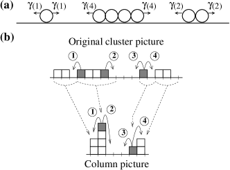
Figure 1: (a) Illustration of the diffusion ($m=1$) and detachment ($m>1$) processes of the model, with the associated rates $\gamma(m)$. (b) Examples of detachment processes (1,2) and diffusion processes (3,4) of shaded particles, in the original cluster picture and in the corresponding column picture. Dashed lines show the correspondence between cluster+vacancy and a column in the two pictures.

At this point, it is also important to recall the differences from previously studied models with similar mechanisms. The case of constant detachment rate (more precisely, $k=0$ and $\gamma_{0}\ll 1$) was considered in Refs. coarsen1 ; chamereis , and shows a coarsening with exponent $z=1/3$ up to a characteristic time of order ${\gamma_{0}}^{-5/2}$. Models with $\gamma(m)$ increasing with $m$ were also analyzed in previous work gama and have prospective application to island formation in heteroepitaxy, particularly due to the possibility of changing the shape of the island size distributions (from monotonic to peaked ones) by tuning temperature or coverage. In those cases, steady states could be attained in infinitely large lattices, but the present model (decreasing $\gamma(m)$) shows a steady state only in a finite lattice. The properties of this steady state can be exactly predicted from a mapping onto a ZRP: for any rate of the form in Eq.(1), there is condensation into a single cluster whose density tends to $1$ as the lattice size increases evanshanney .

Our results for the average cluster sizes, including the logarithmic corrections to the dominant behavior, will be derived from a scaling theory presented in Sec. II and will be confirmed by simulation data. In Sec. IV, we will write the Master equation of the process in an independent interval approximation (IIA), and obtain some exponent relations. However, because of its neglect of important correlations, some results of this IIA do not agree with the scaling ones. But, after some adjustment it is able to predict the correct dominant coarsening exponent. The simulation results for cluster size distributions are shown in Sec. V, which qualitatively confirm the assymmetry predicted by the IIA and the proposed scaling relations for small and for typically large clusters. Finally, in Sec. VI, we present our conclusions.

II Scaling theory

II.1 Basic definitions and coarsening with constant detachment rates

Here we review the heuristic scaling approach based on random walk properties used to predict the time evolution of the typical cluster size. We consider the model with small mass-independent detachment rates, i. e. $\gamma(m)=\gamma_{0}\ll 1$ for $m\geq 2$, while $\gamma(1)=1$ (free particle diffusion). These arguments were formerly presented in Ref. coarsen1 and follow similar lines of those applied to other ZRP in Refs. grobkinsky ; evanshanney . We denote the typical cluster size as $M$, which must be understood as an average over the largest (time-increasing) sizes which are statistically relevant. This average excludes, for instance, clusters with size of order $1$, even if their statistical weights are large.

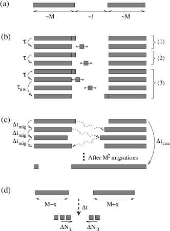
Figure 2: (a) Configuration of two neighboring large clusters with typical size $M$, separated by an empty region of size $l$. (b) Scheme with a sequence of configurations during the migration of a particle from the left to the right cluster. (c) Scheme with successive migrations of particles from one cluster to the other, until the right cluster doubles its mass at the expense of the left one. (d) Scheme with the number of particles ${\Delta N}_{L}$ and ${\Delta N}_{R}$ detached from neighboring clusters during a time interval $\Delta t$. From the model rules, the smaller cluster (left) loses more particles than the larger one (right).

Fig. 2a shows two neighboring clusters of size $M$ separated by a gap of size $l=rM$, where $r$ is related to the particle density (coverage) $\theta$ by

$$r\equiv\frac{\theta}{1-\theta}.$$ (2)

A characteristic time ${\Delta t}_{coa}$ is that in which such clusters exchange so many particles that one of them approximately doubles its mass at the expense of the other. This time is estimated below.

The time for detachment of a single particle from the edge of a cluster is of order $\tau\sim 1/\gamma_{0}$. However, after detachment it is much more probable for this particle to reattach to that cluster than to diffuse to the other cluster. The probability of traveling a distance $l$ before going back to the original cluster is $1/l$, as determined by the solution of ”the gambler’s ruin problem” feller - see also Refs. coarsen1 ; grobkinsky . This means that the particle will detach and reattach to the original cluster a number of times of order $l$ before migrating to the neighboring cluster. This is illustrated in Fig. 2b, where for simplicity only two unsucessful detachments (i. e. detachment-reattachment), labeled (1) and (2), were shown. Consequently, successful migration of a single particle from one cluster to the other takes place after a time ${\Delta t}_{mig}$ given by

$${\Delta t}_{mig}\sim\tau l\sim rM/\gamma_{0}.$$ (3)

The additional time for random walk of the free particle, $\tau_{RW}$, is negligible during coarsening.

The above reasoning implies that single particle exchange does not depend on the current size of each cluster, but only on their separation $l$, which is kept fixed during the process. This symmetric random exchange is illustrated in Fig. 2c. After the migration time $\tau_{mig}$, the size of each cluster increases or decreases by one unit with equal probability. Thus, in order for the size of one of the clusters to increase from $M$ to $2M$ (and the size of the other cluster to decrease from $M$ to zero), the exchange of nearly $M^{2}$ particles is necessary. Thus, the coarsening time is

$${\Delta t}_{coa}\sim M^{2}{\Delta t}_{mig}\sim rM^{3}/\gamma_{0}.$$ (4)

This gives a scaling equation

$$\frac{dM}{dt}\sim\frac{M}{{\Delta t}_{coa}},$$ (5)

from which we obtain

$$M\sim{\left(\frac{\gamma_{0}}{r}t\right)}^{1/3}.$$ (6)

Notice that the random walk of the free particle between the neighboring clusters takes a time of order

$$\tau_{RW}\sim l^{2}\sim{\left(rM\right)}^{2}.$$ (7)

If $\tau_{RW}\ll\tau$, then during the successful migration time there will be only one free particle between the clusters, as assumed above. Otherwise, if $\tau_{RW}\sim\tau$, it is probable that two free particles meet, which leads to the formation of an intermediate cluster with those particles. Since the time necessary for the small intermediate cluster to break is of the same order as the detachment rates from the big clusters ($\tau\sim 1/\gamma_{0}$), the coarsening process ends. In this situation, we have $M\sim\frac{1}{r{\gamma_{0}}^{1/2}}$ for the average cluster size coarsen1 .

II.2 Coarsening with decreasing detachment rates

Here we extend the previous approach to the case of decreasing detachment rates (Eq. 1). In this case, the characteristic time for single particle detachment from a typical cluster of size $M$ is

$$\tau(M)\sim\frac{1}{\gamma\left(M\right)}\sim\frac{M^{k}}{\gamma_{0}},$$ (8)

where we used $\gamma_{0}\sim 1$.

In contrast to the model with constant detachment rates (Sec. II.1), here we observe that coarsening will not end in an infinitely large lattice because, during the exchange of particles between neighboring clusters, the time necessary to break the intermediate cluster is of order $1$, which is much smaller than the detachment time. In a finite lattice, this leads to condensation of a finite fraction of the particles into a single cluster (with the present rates, this fraction tends to $1$ as the size increases) evanshanney .

The time for successful migration from one cluster to the neighboring one is

$${\Delta t}_{mig}\sim\tau l\sim rM^{k+1}/\gamma_{0},$$ (9)

which now depends explicitly on the mass of the cluster from which it detached. Detachment from large clusters is slower, thus there is a preferential flux of particles from small to large neighboring clusters. Eq. (4) is no longer valid because the number of single particle exchanges necessary for two clusters to coarsen is much smaller than $M^{2}$. When the neighboring clusters have nearly the same size, random exchange of particles takes place, but as soon as the sizes are unbalanced the net flux becomes asymmetric.

The next step is to calculate the number of exchanged particles within a time interval $\Delta t$ if the mass is unbalanced by an amount $x$, as shown in Fig. 2d. The numbers of detached particles from the left and the right clusters during that time are, respectively,

$${\Delta N}_{L} \sim \frac{\Delta t}{{\Delta t}_{mig}^{(LEFT)}}\sim\gamma\left(M-x\right)\Delta t/\left(rM\right),$$

$${\Delta N}_{R} \sim \frac{\Delta t}{{\Delta t}_{mig}^{(RIGHT)}}\sim\gamma\left(M+x\right)\Delta t/\left(rM\right).$$ (10)

Consequently, the mass difference $x$ increases by

$$\Delta x={\Delta N}_{L}-{\Delta N}_{R}\sim\frac{\gamma_{0}}{rM^{k+1}}\left[{\left(1-\frac{x}{M}\right)}^{-k}-{\left(1+\frac{x}{M}\right)}^{-k}\right]{\Delta t}$$ (11)

within time $\Delta t$.

The time for a net flux of a fixed mass $\Delta x$ decreases as $x$ increases, which means slow coarsening for clusters of nearly the same size and rapid coarsening with one big and one small cluster. Transfer of unit mass ($\Delta x=1$) takes place in a time of order

$${\Delta t}_{1}\sim\frac{rM^{k+1}}{\gamma_{0}}{\left[{\left(1-\frac{x}{M}\right)}^{-k}-{\left(1+\frac{x}{M}\right)}^{-k}\right]}^{-1}$$ (12)

and the coarsening time is

$${\Delta t}_{coa}=\sum_{x=1}^{x=M}{{\Delta t}_{1}}\sim\frac{rM^{k+2}}{\gamma_{0}}\int_{1/M}^{1}{\frac{du}{{\left(1-u\right)}^{-k}-{\left(1+u\right)}^{-k}}}$$ (13)

For typical masses $M\gg 1$, the integral in Eq. (13) is dominated by $u\ll 1$, where ${\left(1-u\right)}^{-k}-{\left(1+u\right)}^{-k}\approx 2ku+{\cal O}\left(u^{3}\right)$. Since we consider $k\sim 1$, we obtain

$${\Delta t}_{coa}\sim\frac{r}{\gamma_{0}}M^{k+2}\ln{M}.$$ (14)

Notice that $u\ll 1$ in Eq. (13), which leads to the logarithmic correction in Eq. (14), physically corresponds to the regime of symmetric particle exchange, i. e. neighboring clusters with approximately the same size. Similar arguments were used to calculate coarsening times in Ref. torok . Since $k>0$, we observe that ${\Delta t}_{coa}$ is always larger than the time for random walk between the clusters, given by Eq. (7), thus particle detachment is always the leading contribution to the coarsening time of large clusters.

Substituting Eq. (14) in the scaling equation (5), we obtain

$$M\sim{\left[\frac{\gamma_{0}}{r}\frac{t}{\ln{t}}\right]}^{z},\qquad z=\frac{1}{k+2}.$$ (15)

In order to test these predictions, we performed numerical simulations of the model for several values of $k$ in the range $[0.25,3]$, with coverages $\theta=0.8$, in lattices of sizes from $L=8192$ to $L=32768$, so that finite-size effects are negligible. Simulations for some smaller coverages were also performed, but the coarsening process usually takes place at much longer times. The average cluster size ${\langle m\rangle}$ was obtained from at least 100 configurations for each $K$, up to times of order $t={10}^{6}$.

Estimates of the exponent $z$ are usually obtained from extrapolation of effective exponents calculated from ${\langle m\rangle}\left(t\right)$. Without accounting for logarithmic corrections in Eq. (15), we define the effective exponents as

$$z_{eff,1}=\frac{\ln{\left[\langle m\rangle\left(t\right)/\langle m\rangle\left(t-\delta t\right)\right]}}{\ln{\left[t/\left(t-\delta t\right)\right]}},$$ (16)

with fixed $\delta t$. On the other hand, in order to account for the logarithmic corrections in Eq. (15), the effective exponents must be defined as

$$z_{eff,2}=\frac{\ln{\left[\langle m\rangle\left(t\right)/\langle m\rangle\left(t-\delta t\right)\right]}}{\ln{\left[\left(t/\ln{t}\right)/\left(\left(t-\delta t\right)/\ln{\left(t-\delta t\right)}\right)\right]}}.$$ (17)

$z_{eff,1}$ is plotted in Fig. 3a as a function of $1/t$ for $k=3$, $k=2$, $k=1$ and $k=0.25$, and $z_{eff,2}$ is plotted in Fig. 3b for the same values of $k$. Predicted asymptotic values $z=1/\left(k+2\right)$ (Eq. 15) are $0.2$, $0.25$, $0.333$ and $0.444$, respectively. For all $k\geq 1$, we observe that convergence to the asymptotic $z$ (as $1/t\to 0$) is faster with $z_{eff,2}$. This justifies the theoretically predicted logarithmic corrections.

However, for $k=0.25$ we observe that both $z_{eff,1}$ and $z_{eff,2}$ converge to $z\approx 0.12$, which is very far from the predicted value of Eq. (15). In Sec. II.3, we will show that for $k<1$ the coarsening exponent for ${\langle m\rangle}$ is actually different from $z=1/(k+2)$ due to the large density of isolated particles. Thus ${\langle m\rangle}$ is very different from $M$, which represents the typical size of large, increasing clusters. However, we will show that $M$ still coarsens with the exponent given by Eq. (15).

Figure 3: (Color online) Effective exponents $z_{eff,1}$ (a) and $z_{eff,2}$ (b) of the average cluster size (average over all clusters) as a function of inverse time, with coverage $\theta=0.8$: $k=3$ (squares), $k=2$ (up triangles), $k=1$ (crosses), and $k=0.25$ (down triangles).

II.3 The role of isolated particles

The successful detachment of a particle from a cluster, which allows the migration to the neighboring one, takes place after a time interval given by Eq. (9). However, this time measures the average residence time of the particle attached to the original cluster. The total time of migration of a single particle has to include the random walk time between the neighboring clusters, which is given by Eq. (7).

If $t_{mig}>\tau_{RW}$, then the random walk is rapid, thus it is very rare to observe a single free particle between any pair of clusters and even rarer to observe two. This condition is satisfied when $k>1$. Fig. 4a shows some snapshots of the simulation for $k=2$, which confirm this behavior. Thus, the large clusters with mass of order $M$ are statistically dominant, i. e. $M$ actually represents the average cluster mass among all clusters, which we denote by $\langle m\rangle$.

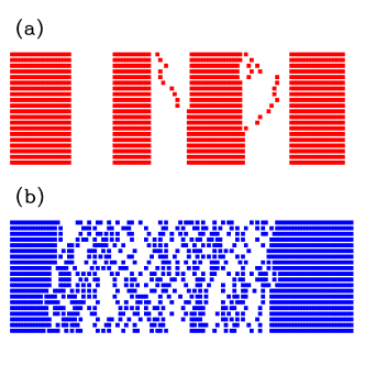
Figure 4: (Color online) Sequences of configurations (from top to bottom) of a certain region of the lattice for (a) $k=2$ and (b) $k=0.5$. In both cases, the coverage is $\theta=0.6$ and snapshots are separated by a time interval $10$ (simulation times are of order ${10}^{4}$).

On the other hand, if $k<1$, a large time is spent in the random walk between neighboring clusters. During this time, the successful detachment of other particles is possible (we recall that intermediate small clusters rapidly break for $\gamma_{0}\sim 1$). This is illustrated for $k=1/2$ in the snapshots of Fig. 4b. The number of free particles during $\tau_{RW}$ in the region between two large clusters is of order

$$N_{1}\sim\tau_{RW}/t_{mig}\sim M^{1-k}$$ (18)

and the corresponding density of free particles is

$$\rho_{1}\sim N_{1}/M\sim M^{-k}.$$ (19)

However, the density of large clusters, whose typical mass is $M$, varies as

$$\rho_{large}\sim 1/M.$$ (20)

This means that the free particles (or small clusters formed by their attachment) are statistically dominant for $k<1$. In this situation, $M$ represents the average size of large clusters, but not the average size among all clusters, which is $\langle m\rangle$.

For $k>1$, Eq. (19) is also valid as a density averaged in space and time (during most of the time, there is no free particle between the neighboring clusters), thus large clusters of size $M$ are statistically dominant and $\langle m\rangle\approx M$.

These results do not invalidate the arguments of Sec. II.1 for the scaling of $M$, which is still expected to follow Eq. (15) for $k<1$. The average cluster size calculated among all clusters, including free particles, is obtained from an average in the region between two large clusters:

$$\langle m\rangle\sim\frac{1\cdot N_{1}+M\cdot 1}{N_{1}+1}\sim\frac{M}{1+M^{1-k}}.$$ (21)

With $k<1$, this global average scales as

$$\langle m\rangle\sim M^{k}\sim{\left(\frac{t}{\ln{t}}\right)}^{z_{G}},\qquad z_{G}=\frac{k}{k+2}\qquad(k<1).$$ (22)

This explains the discrepancies in the numerical estimates of coarsening exponents for $k<1$ (Sec. II.2). For instance, for $k=0.25$, Eq. (22) predicts $z_{G}=0.111$, which is consistent with the trend of the data in Figs. 3a and 3b.

In order to test the predicted scaling of $M(t)$, we calculated numerically average cluster sizes from contributions of large clusters only (masses $m>12$ for $k=0.5$, $m>25$ for $k=0.25$). Corresponding effective exponents are defined as

$$z_{eff,3}=\frac{\ln{\left[M\left(t\right)/M\left(t-\delta t\right)\right]}}{\ln{\left[\left(t/\ln{t}\right)/\left(\left(t-\delta t\right)/\ln{\left(t-\delta t\right)}\right)\right]}}.$$ (23)

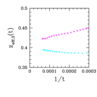
Figure 5: (Color online) Effective exponents $z_{eff,3}$ for average cluster sizes excluding small clusters, with coverage $\theta=0.8$: $k=0.5$ (asterisks) and $k=0.25$ (down triangles).

$z_{eff,3}$ is shown in Fig. 5 as a function of $1/t$ for $k=0.25$ and $k=0.5$. Good agreement with the predicted asymptotic value $z=0.4$ for $k=0.5$ is obtained. For $k=0.25$, the trend of $z_{eff,3}$ as $1/t\to 0$ is not consistent with the predicted value $0.444$, which is probably due to corrections to scaling. In both cases, effective exponents not accounting for the logarithmic corrections (similarly to $z_{eff,1}$ - Eq. 16) show larger discrepancies from the theoretically predicted values of $z$.

Additional support to our theoretical predictions is provided by the numerical study of the scaling of the density of free particles. From Eqs. (15) and (18), we obtain

$$\rho_{1}\sim{\left(\frac{t}{\ln{t}}\right)}^{-z\left(1\right)},$$ (24)

with

$$z\left(1\right)=\frac{k}{k+2}.$$ (25)

(i. e. $z\left(1\right)=z_{G}$ for $k<1$). In Fig. 6 we show ${\left[t/\ln{\left(t\right)}\right]}^{z\left(1\right)}\rho_{1}$ versus $1/t$ for $k=2$, $k=1$ and $k=1/2$, using the exponents $z(1)$ given by Eq. (25). The convergence of that ratio to finite non-zero values as $t\to\infty$ confirms the expected scaling.

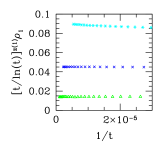
Figure 6: (Color online) Simulation results for the scaled density of isolated particles as a function of inverse time, with coverage $\theta=0.8$: $k=2$ (triangles), $k=1$ (crosses) and $k=0.5$ (asterisks).

The densities of other small clusters can be obtained from $\rho_{1}$ by observing that they have high detachement rates and, consequently, they may be viewed as a set of nearly free particles at consecutive lattice sites. This reasoning gives the density of clusters of size $m$, for $m\sim 1$ as

$$\rho_{m}\sim{\left(\rho_{1}\right)}^{m}\sim{\left(\frac{t}{\ln{t}}\right)}^{-z\left(m\right)},$$ (26)

with

$$z\left(m\right)=mz\left(1\right).$$ (27)

Simulations also confirm this result for small clusters, such as $m=2$ and $m=3$, for several values of $k$.

III Relation to other models

Our model may be mapped onto a column problem which clearly shows that it is a ZRP. A cluster of length $m$ in the original problem and the vacant site at its right side is represented by a column of mass $m$ in this new picture. The mapping is illustrated in Fig. 1b. Sets of $n$ consecutive vacancies in the original problem are represented by $n-1$ vacant columns in the new picture. The detachment and diffusion processes correspond to hopping of a particle from a column to the neighboring one. The mass-dependence of detachment rates is translated into mass-dependent hopping rates $\gamma(m)=2\epsilon(m)$ in order to account for the detachment in two edges of each cluster, each one with rate $\epsilon(m)$.

In a finite lattice, condensation of a finite fraction of the mass in a single cluster is expected for all densities if $\gamma(m)\to 0$ for $m\to\infty$. Moreover, the density of particles out of the condensate decreases as $L\to\infty$, as explained in Ref. evanshanney . This is the case of our model, and our simulations in small lattices confirm those steady state features.

However, while steady state properties of ZRP can be analytically calculated, the coarsening process in infinitely large lattices is much more difficult to predict. That is the reason why we use scaling approaches, simulation and analytical tools based on suitable approximations (Sec. IV) to study coarsening of our model.

Comparison with related models is interesting at this point. Godréche godreche and Gro$\beta$kinsky et al grobkinsky analyzed the ZRP with hopping rates $\gamma(m)=1+b/m$ using heuristic arguments similar to ours (see also review in Ref. evanshanney ). They considered the cases of symmetric and asymmetric hopping rates, which lead to average cluster size scaling as $\langle m\rangle\sim t^{1/3}$ and $\langle m\rangle\sim t^{1/2}$, respectively. The symmetric case is somehow equivalent to our model with mass-independent detachment rates (Sec. II.1), since both have constant and nonzero $\gamma(m)$ for $m\to\infty$ (very large clusters).

However, it is important to notice that our model with $k\to 0$, i. e. with very weak mass-dependence of hopping rates, has $z\to 1/2$, in contrast to $z=1/3$ which characterizes constant detachment rates. Both models consider symmetric hopping rates, but the asymmetric flux of mass between the neighboring clusters in our model is always present and is responsible for the faster coarsening, even if $k$ is very small. In other words, coarsening in the model with $k\to 0$ is very different from that with $k=0$.

On the other hand, we note that $z=1/3$ is obtained in our model for $k=1$. In this case, the detachment rates decreasing with cluster size tend to make the coarsening slower, and balances the effect of the asymmetric particle flux between clusters, which favors faster coarsening. For $k>1$, mechanisms favoring slow coarsening are stronger, thus $z<1/3$. For $k<1$, mechanisms favoring fast coarsening are stronger, thus $z>1/3$. However, both mechanisms are absent in the model with constant $\gamma$ and in the model of Gro$\beta$kinsky et al grobkinsky , both having $z=1/3$.

The above discussion leads to the the conclusion that the same exponents may be obtained with different microscopic dynamics, while apparently similar dynamics may lead to very different coarsening exponents. It is important that such features are considered if one aims to model real systems by ZRP or similar models.

IV Independent interval approximation

IV.1 General formulation

The full analytic description of systems with stochastic processes such as those of our model is provided by the Master equation, which is most easily written in the column picture of Fig. 1b. Previously, this approach was used to study the (exact) steady states of related models which correspond to ZRP coarsen1 ; gama and the coarsening in models with increasing number of particles due to deposition processes coarsen2 .

The description of the present model is simplified by the fact that the process conserves the total particle numbers $N$. Thus, using periodic boundary conditions and a total number of sites $L$ (lattice length in the original cluster picture), and denoting by $N_{t}(m)$ the total number of clusters of size $m$ ($\geq 1$) at time $t$, it follows that (i) $N=\sum_{m=1}^{\infty}{mN_{t}(m)}$, (ii) the number of spacers in the column picture is $\sum_{m=1}^{\infty}{N_{t}(m)}$, and (iii) $N_{t}(m)$ equals the number of columns of size $m$, for $m>0$. Hence, denoting by $N_{t}(0)$ the number of columns of size zero, we have $\sum_{m=0}^{\infty}{N_{t}(m)}=L-N\equiv L(1-\theta)$ (the last step defining the coverage $\theta$ in the original picture). Thus the total number of columns (including those of size zero) is a constant $L_{c}=L-N$. The density in the column picture is $\rho_{c}\equiv N/L_{c}=r$ (Eq. 2).

The system configuration can be specified by the ordered set of numbers of particles in each of the columns in succession: $\left(m_{1},m_{2}\dots m_{L_{c}}\right)=\{m_{i}\}$. The probability $P_{t}\{m_{i}\}$ at time $t$ of the configuration $\{m_{i}\}$ changes by in and out processes. Collecting the effects of all such processes in a time step $t\to t+1$ (see e. g. Refs. coarsen1 ; gama ) gives the full Master equation

$$P_{t+1}\{m_{i}\}-P_{t}\{m_{i}\}=$$

$$\sum_{l=1}^{L}[\gamma\left(m_{l-1}+1\right)P_{t}\left(\dots m_{l-1}+1,m_{l}-1\dots\right)$$

$$+\gamma\left(m_{l+1}+1\right)P_{t}\left(\dots m_{l}-1,m_{l+1}+1\dots\right)$$

$$-2\gamma\left(m_{l}\right)P_{t}\{m_{i}\}]\theta\left(m_{l}\right).$$ (28)

The theta function above (zero for $m\leq 0$, otherwise unity) is actually redundant as $P_{t}\left(\dots m-1\dots\right)$ and $\gamma(m)$ vanish for $m\leq 0$.

The Independent Interval Approximation (IIA) assumes that the configuration probability $P_{t}\{m_{i}\}$ can be factorised as $\prod_{l=1}^{L-N}{P_{t,l}\left(m_{l}\right)}$. That leads to a reduced form of the Master equation in which cluster-cluster correlations are neglected:

$$P_{t+1,l}\left(m\right)-P_{t,l}\left(m\right)={\cal A}_{t}\left(m+1,l\right)-{\cal A}_{t}\left(m,l\right),$$ (29)

where

$${\cal A}_{t}\left(m,l\right) \equiv P_{t,l}\left(m\right)\gamma\left(m\right)\Theta\left(m-1\right)+\delta_{m,1}\gamma\left(1\right)P_{t,l}\left(1\right)$$ (30)

$$-\left[P_{t,l}\left(m-1\right)\Theta\left(m-1\right)+\delta_{m,1}P_{t,l}\left(0\right)\right]{\cal J}\left(l\right)$$

$$= \Theta\left(m\right)A_{t}\left(m,l\right),$$

with

$$A_{t}\left(m,l\right)=P_{t,l}\left(m\right)\gamma\left(m\right)-P_{t,l}\left(m-1\right){\cal J}\left(l\right),$$ (31)

and

$${\cal J}\left(l\right)\equiv\sum_{m=1}^{\infty}{\frac{1}{2}\gamma\left(m\right)\left[P_{t,l-1}\left(m\right)+P_{t,l+1}\left(m\right)\right]}.$$ (32)

In Eq. (30), the Theta function $\Theta(m)$ is zero for $m\leq 0$, otherwise it is unity. A further reduction results from neglecting dependences on the column label $l$, so $P_{tl}\left(m\right)$ becomes $P_{t}\left(m\right)$. This form of IIA gives

$$P_{t+1}\left(m\right)-P_{t}\left(m\right)=A_{t}\left(m+1\right)-A_{t}\left(m\right)\Theta\left(m\right),$$ (33)

where

$$A_{t}\left(m\right)=P_{t}\left(m\right)\gamma\left(m\right)-\Gamma_{t}P_{t}\left(m-1\right),m\geq 1,$$ (34)

and

$$\Gamma_{t}=\sum_{m-1}^{\infty}{\gamma\left(m\right)P_{t}\left(m\right)}.$$ (35)

A useful result from the IIA equation (33) for large masses $m$ is

$$\sum_{m^{\prime}=m}^{\infty}{P_{t}\left(m^{\prime}\right)-P_{t+1}\left(m^{\prime}\right)}=A_{t}\left(m\right).$$ (36)

Hereafter we consider the mass-dependent rates in Eq. (1) for $m\geq 1$. Unless otherwise stated, we will proceed with developments without dependence on column label $l$, i. e. starting from Eqs. (33), (34), (35) and (36), with $\sum_{m=0}^{\infty}{P_{t}\left(m\right)}=1$. Notice that $P_{t}\left(m\right)$ here differs from the density $\rho_{m}$ in Sec. (II) by a constant factor $1-\theta$ due to the different lattice lengths used to normalize probabilities in different pictures.

IV.2 Scaling characteristics

The late time coarsening of large characteristic masses is expected to be described by

$$P_{t}\left(m\right)\sim\frac{1}{t^{y}}f\left(\frac{m}{t^{z}}\right).$$ (37)

The exponents $y$ and $z$ depend on $k$, and $y$ need not equal $z$ because the large masses need not dominate the normalisation sums, as shown in Sec. II.3. The region of the cluster size distribution where the scaling equation (37) applies and masses are of order $t^{z}$ is hereafter called region S.

For small $m$, we have

$$P_{t}\left(m\right)\sim t^{-z\left(m\right)},m\ll t^{z},$$ (38)

where $z(m)$ is defined consistently with Eq. (26). This region is hereafter denoted as A.

Finally, $P_{t}\left(0\right)$ may strongly contribute to normalisation sums because, as coarsening continues and $P(m)$ at small $m$ decreases, $P_{t}(0)$ will approach $1$. So, at late times,

$$1-P_{t}\left(0\right)\sim t^{-z_{A}},$$ (39)

which defines $z_{A}$.

IV.3 Direct results for small clusters

The IIA equations and the above definitions and properties directly lead to some results for small $m$ and large times. This is a quasistatic situation in which probabilities slowly vary in time, thus the left hand side (LHS) of Eq. (33) is negligible. Since Eq. (33) is valid for all $m\geq 0$ this leads to $A_{t}(m)\sim 0$, and Eq. (34) leads to

$$P_{t}\left(m\right)\sim P_{t}\left(0\right){\Gamma_{t}}^{m}{\left(m!\right)}^{k}.$$ (40)

Since $P_{t}\left(0\right)\sim 1$, this yelds the form (38) and confirms the relation (27) among the coarsening exponents of small $m$ given that

$$\Gamma_{t}\propto t^{-z\left(1\right)}.$$ (41)

The sizes of the terms on the LHS and on the right hand side of Eq. (33) are respectively, for a given $m$, of order $(d/dt)\left[P_{t}\left(m\right)\right]\sim t^{-1-z\left(m\right)}=t^{-1-mz\left(1\right)}$ and $A_{t}\left(m+1\right)\sim t^{-z\left(m+1\right)}=t^{-\left(m+1\right)z\left(1\right)}$. The quasistatic assumption means that the former is negligible compared to the latter quantity at long times, thus

$$z\left(1\right)<1.$$ (42)

This result is also consistent with the scaling picture of Sec. II and simulation results.

The sum in Eq. (35) can then be separated into the contributions from the two regions, A and S. Eqs. (38) and (41) [with (27)] apply to A and Eq. (37) applies to S, thus

$$\Gamma_{t} \sim \sum_{m=1}^{m_{0}\left(t\right)}{\left[\dots t^{-mz\left(1\right)}\gamma\left(m\right)\right]}+\int_{m_{0}\left(t\right)}^{\infty}{m^{-k}t^{-y}f\left(\frac{m}{t^{z}}\right)dm}$$ (43)

$$\sim \dots t^{-z\left(1\right)}+\dots+t^{-\left[y+\left(k-1\right)z\right]},$$

with $1\ll m_{0}\left(t\right)\ll t^{z}$. Eq. (43) is consistent with (41) if

$$z\left(1\right)\leq y+\left(k-1\right)z.$$ (44)

Simulations strongly support Eqs. (41) and (43), as well as (44) as an inequality (which is also consistent with the scaling theory, as discussed below). This implies that the sum in $\Gamma_{t}$ is dominated by the small $m$ region (actually by just the $m=1$ term). The result (40), which implies $P_{t}\left(m\right)/{\left[P_{t}\left(1\right)\right]}^{m}={\left(m\right)}^{k}$, is also confirmed by simulation.

IV.4 Results for large clusters and exponents relations

Here we denote by $\sum_{A}$ and $\sum_{S}$ the summations with respect to $m$ over regions A and S, respectively.

Consider the sum giving the density in the column picture

$$\rho_{c} = \sum_{m=1}^{\infty}{mP_{t}\left(m\right)}=$$ (45)

$$\sum_{A}{mP_{t}\left(m\right)}+\sum_{S}{mP_{t}\left(m\right)}=$$

$$\dots t^{-z\left(1\right)}+\dots t^{-\left(y-2z\right)}$$

(the sums being carried out in same way as those giving Eq. 43). Since $\rho_{c}$ is constant in time, this is consistent with

$$y=2z.$$ (46)

Similarly, the density of clusters in the scaling region S is

$$\sum_{S}{P_{t}\left(m\right)}\propto t^{-\left(y-z\right)}\propto t^{-z},$$ (47)

where we used Eq. (46).

A further exponent relation follows from Eq. (39) and

$$1-P_{t}\left(0\right) = \sum_{A}{P_{t}\left(m\right)}+\sum_{S}{P_{t}\left(m\right)}=$$ (48)

$$\dots t^{-z\left(1\right)}+\dots t^{-z}=\dots t^{z_{A}},$$

which gives

$$z_{A}=min\{z\left(1\right),z\}.$$ (49)

It turns out that the minumum here is $z(1)$ for $k<1$ and $z$ for $k\geq 1$, where small and large clusters are respectively dominant (this was shown in Sec. II and will be confirmed in the context of the IIA below).

These considerations warns us that there are several average masses, including

$$\sum_{S}{mP_{t}\left(m\right)}/\sum_{S}{P_{t}\left(m\right)}\propto$$

$$t^{z}\sum_{m=1}^{\infty}{mP_{t}\left(m\right)}/\sum_{m=1}^{\infty}{P_{t}\left(m\right)}\propto t^{z_{A}},$$ (50)

with $z_{A}$ given by Eq. (49).

Now consider the IIA Master equation in the form Eq. (36), and the ansatz for the scaling regime, Eq. (37). Replacing the time difference by a derivative and the sum over $m$ by an integral, we have (also using Eqs. 1, 34 and 41)

$$\int_{m}^{\infty}{dm^{\prime}\frac{\partial}{\partial t}\left[t^{-y}f\left(\frac{m^{\prime}}{t^{z}}\right)\right]}=$$

$$\left[\dots m^{-k}-\dots t^{-z\left(1\right)}\left(1-\frac{\partial}{\partial m}\right)\right]t^{-y}f\left(\frac{m}{t^{z}}\right).$$ (51)

The leading order terms on the RHS cannot cancel, since they have different dependences on $m$, so we can ignore the subdominant $\frac{\partial}{\partial m}$ (which came from the $m-1$ argument). With $x\equiv m/t^{z}$ and $u=m^{\prime}/t^{z}$, the result is

$$-t^{z-y-1}\int_{x}^{\infty}{du\left[yf\left(u\right)+zuf^{\prime}\left(u\right)\right]}=$$

$$\left[\dots t^{-zk}x^{-k}-\dots t^{-z\left(1\right)}\right]t^{-y}f\left(x\right).$$ (52)

The quasi-static results for small $m$ came from achieving a cancellation on the RHS. For the large $m$ case, the different $x$-dependences preclude cancellation, but both terms on the RHS have the same dominant order if Eq. (25) is valid. As shown in Sec. II, this is consistent with our scaling theory and with simulation data.

However, the dominant $t$-dependences in the LHS and RHS of Eq. (52) give

$$z-y-1=-zk-y\qquad\Rightarrow\qquad z=\frac{1}{k+1}.$$ (53)

Comparison with $z=\frac{1}{k+2}$, given by Eq. (15) and confirmed by simulation, shows that this result is not correct. The origin of the discrepancy is an important correlation missed by the IIA, as will be discussed below.

IV.5 Inadequacy of the IIA and a heuristic adjustment

The temporal evolution at large $m$ is being misrepresented by the IIA because it associates a product weight $P_{t}\left(m\right)P_{t}\left(1\right)$ to the joint occurrence of a free particle and a cluster of mass $m$, not distinguishing between cases where the particle and the cluster are adjacent or well separated. These two cases are very different for large $m$ because of the small probability of detachment of a particle from a large cluster and the high probability of the subsequent random walk of the particle finishing with absorption at the originating cluster. In the full original Master equation [Eq. (28), with cluster/column labels and without factorisation of probabilities] it is easy to identify the random walk steps (through the $i$-labels, and since they occur with rate $\gamma(1)$). For comparison, we can also see them through $A_{t}\left(m,l\right)$ in the IIA version retaining column labels [Eqs. (29), (30), (31) and (32)], where here the inadequate factorisation has been made (which does not properly represent the distortion of the walk by the large cluster).

These problems can be adjusted as follows. The absorbing aspect of the random walk of a single particle near a large cluster reduces the effective rate of migration to another large cluster. Given that their average separation increases as their average size, $t^{z}$, the reduction is by an extra factor $t^{-z}$, to be introduced into the terms on the RHS of Eq. (51) (consequently, the RHS of Eq. 52 also changes by the extra factor $t^{-z}$). This is equivalent to the effect included in the scaling arguments of Sec. II. The consequence is that in place of Eq. (53), the power counting gives

$$z-y-1=-zk-y-z\qquad\Rightarrow\qquad z=\frac{1}{k+2}.$$ (54)

The extra factors $t^{-z}$ do not modify the quasi-static form for the distribution function $P_{t}(m)$ at small $m$, thus its introduction is still consistent with Eq. (25).

Thus, using these heuristic arguments we are able to predict the correct coarsening exponent and preserve several exponents relations. However, the changes are still unable to predict the logarithmic corrections shown in Sec. II.2, which are related to a crossover from symmetric to asymmetric particle exchange between neighboring clusters.

IV.6 Cluster size distributions

Using Eqs. (25) and (41), the quasistatic result (40) for small masses can be rewritten as

$$P_{t}\left(m\right)\sim{\left(\frac{m}{t^{z}}e\right)}^{mk}.$$ (55)

Comparing with $t^{-y}f\left(\frac{m}{t^{z}}\right)$ (Eq. 37), it can be estimated that the crossover between the forms for the region A and the scaling region S occurs at $m=m_{0}(t)$ where

$$m_{0}(t)\sim\frac{1}{e}t^{z}\left[1+{\cal O}\left(t^{-z}\ln{t}\right)\right].$$ (56)

The form (55) first decreases with $m$ (due to the increasing power of $t^{-z}$) but then turns over into an increasing function when $m$ exceeds ${\cal O}\left(t^{z}\right)$. The minimum is at $m=\overline{m}\left(t\right)$ such that $0=\frac{d}{dm}\left[\ln{P\left(m\right)}\right]\sim\frac{d}{dm}\left[mk\left(\ln{m}-z\ln{t}-1\right)\right]=k\left(\ln{m}-x\ln{t}\right)$, so

$$\overline{m}\left(t\right)=t^{z}.$$ (57)

Thus the minimum is near the crossover region. Simulations consistently show that the scaling starts just beyond the minimum and that the quasistatic results (40) and (55) work well up to just beyond the minimum.

Eqs. (15) and (57) imply that the position of the minimum decreaases with increasing $k$. This is also seen in simulations, and is consistent with small clusters having largely $m=1$ for $k>1$ and a greater spread for $k<1$.

The adjusted form of Eq. (52) for the scaling function (Sec. IV.5) is, using Eqs. (25) and (46),

$$-\int_{x}^{\infty}{du\left[2f\left(u\right)+uf^{\prime}\left(u\right)\right]}=\left(ax^{-k}-b\right)f\left(x\right)$$ (58)

where the factors of $t$ have consistently cancelled by using the correct coarsening exponent (Eq. 54), and $a$ and $b$ are constants associated with $\gamma(m)$ and $\Gamma$, respectively. Differentiating Eq. (58) with respect to $x$ gives $-\frac{d\ln{f\left(x\right)}}{dx}=\frac{2-akx^{-\left(k+1\right)}}{x+ax^{-k}-b}$, hence

$$f\left(x\right)\propto\exp\left[-\int{dx\frac{2-akx^{-\left(k+1\right)}}{x+ax^{-k}-b}}\right].$$ (59)

For small $x$, the integrand in the indefinite integral is dominated by $-kx^{-\left(k+1\right)}/x^{-k}$, which integrates to $\ln{x^{-k}}$, thus

$$f\left(x\right)\propto x^{k}.$$ (60)

For large $x$, the dominant part of the integrand is $2/x$, giving

$$f\left(x\right)\propto x^{-2}.$$ (61)

V Simulation results for cluster size distributions

Despite the problems of the IIA to predict the coarsening exponents and the absence of the logarithmic corrections in the time scaling, even after suitable adjustment (Sec. IV.5), it progresses beyond the previous scaling theory (Sec. II) by providing information on the cluster size distributions, which can now be compared to simulation data.

The unusual shape of the cluster size distribution in this problem is illustrated in Fig. 7 for $k=1$ ($t=5\times{10}^{5}$) and $k=0.5$ ($t={10}^{6}$). There is a rapid (power-law) decrease of $P(m)$ for small $m$, usually until $m$ of order $10$, and a peak appears at large $m$, i. e. in the range of typical large clusters. For $k>1$, the statistical weight of the small clusters decreases with time, i. e. the left side of the curve becomes smaller when compared to the peaked region. For $k<1$ the opposite occurs: as time increases, the weight of the small $m$ region increases and the peak becomes relatively smaller. Indeed, the curve for $k=1/2$ in Fig. 7 shows that the probability of isolated particles or dimers is $100$ to $1000$ times larger than the probability of sizes in the peaked region [for instance, $P(1)\approx 0.77$].

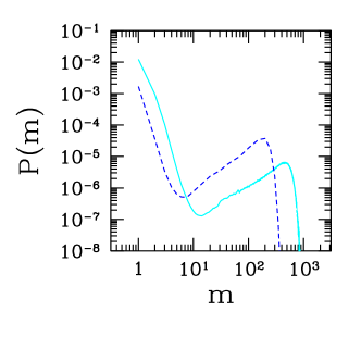
Figure 7: (Color online) Cluster size distributions for $k=1$ at $t=5\times{10}^{5}$ (dashed curve) and $k=0.5$ at $t={10}^{6}$ (solid curve).

The first important result of the IIA is Eq. (37) for the scaling region (the region of the peak in Fig. 7), with $y$ given by Eq. (46). Simulations show that this result is valid with $t$ replaced by $t_{l}=t/\ln{t}$, which is an expected correction. This is illustrated in Figs. 8a and 8b, where we show $\log{\left[t_{l}^{y}P_{t}\left(m\right)\right]}$ as a function of $m/{t_{l}}^{z}$ for $k=0.5$ and $k=2$, respectively, and three different times for each $k$. The good data collapse (particularly for the largest times) is obtained with $z=1/\left(k+2\right)$ and $y=2z$, as predicted by Eqs. (15) and (46).

A power-law in the left tail of the scaling function $f(x)$ is observed in our simulations, but the exponents are different from those predicted in Eq. (60) for small $k$. For instance, for $k=0.5$, the exponent is $1.07$. For larger $k$, the agreement is slightly better, e. g. exponent $2.05$ for $k=2$. Anyway, one interesting feature of the IIA results (60) and (61) is that the left tails of the distributions are heavier than their right tails for $k<2$. In other words, the distributions have negative skewness. This is clearly observed in Fig. 8a, for $k=0.5$, while for $k=2$ (Fig. 8b) the skewness is closer to zero (but still negative).

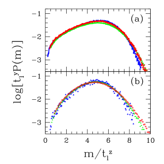
Figure 8: (Color online) Scaled cluster size distributions in the scaling region for: (a) $k=0.5$ at $t={10}^{5}$ (crosses), $t=2\times{10}^{5}$ (squares) and $t={10}^{6}$ (triangles); (b) $k=2$ at $t=2\times{10}^{5}$ (squares), $t={10}^{6}$ (crosses) and $t=5\times{10}^{6}$ (triangles).

The negative skewness of cluster size distributions is an uncommon feature in this type of problem in one dimension; for instance, the distributions in coarsening with constant detachment rates are positively skewed chamereis , as well as those in the steady states with some rate functions which increase with cluster size (due e. g. to repulsive interactions) gama . Thus, in a real system, that feature would suggest the presence of attractive interactions leading to a decrease of the detachement rate with cluster size. On the other hand, it is important to notice that it is a common feature in two dimensions, both in point islands models (which are two-dimensional ZRP) and in extended islands models etb .

The scaling of small masses (Eq. 55) is confirmed in Figs. 9a and 9b for the same values of $k$, again with the logarithmic corrections in the time $t$. There we plot $\log{\left[P_{t}\left(m\right)\right]}$ versus $m\log{\left(m/t^{z}\right)}$, which is proportional to the logarithm of the RHS of Eq. (55). In Figs. 9a and 9b, one important point is the large range of both variables (horizontal and vertical), which span 2 to 6 orders of magnitude. This explains the discrepancies from a perfect data collapse when compared to the scaling regime in Figs. 8a and 8b.

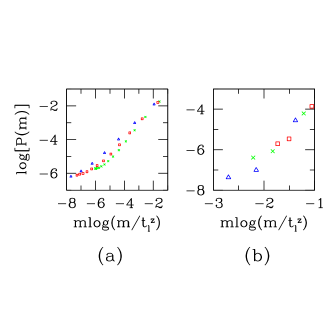
Figure 9: (Color online) Scaled cluster size distributions in the small mass region for(a) $k=0.5$ and (b) $k=2$. Symbols are the same of Figs. 9a and 9b.

VI Conclusion

We studied conserved one-dimensional models of particle diffusion, attachment and detachment from clusters, where the detachment rates decrease with increasing cluster size as $\gamma(m)\sim m^{-k}$. Heuristic scaling arguments based on random walk properties were used to predict the scaling of the typical cluster size as ${\left(t/\ln{t}\right)}^{z}$, with $z=1/\left(k+2\right)$. The coarsening of neighboring clusters is characterized by initial symmetric flux of particles between them followed by an effectively assymmetric flux due to the unbalanced detachment rates (despite the symmetric model rules). For $k<1$, the average cluster size does not scale as the size of typically large clusters due to the high densities of small clusters, which dominate that average. We also solve the Master equation of the model under an independent interval approximation, which predicts some exponent relations and the correct dominant coarsening exponent after suitable changes to incorporate effects of correlations. These results are confirmed by simulation, which also shows the negatively skewed cluster size distributions (particularly for small $k$) and the different scaling relations followed by small clusters (sizes of order $1$) and by typically large clusters (size of order $t^{z}$).

The rate functions analyzed here may arise from associating (Arrhenius) detachment rates with potentials $U(m)$ for particles at the end of a cluster of size $m$. $U(m)$ is then a sum, from $l=1$ to $m-1$, of pair potentials $V(l)$ for separation $l$ with Coulomb-like (inverse of distance) attractive form. In a real system, such interaction is not expected to be valid for all sizes, but may be a reasonable approximation for some ranges, in a similar way that long range repulsion between adatoms on a surface represents substrate-mediated interactions. The particular coarsening features discussed here will certainly help to identify such application.

It is also interesting to note that our model with $\gamma(m)\sim\exp{\left(-m^{2}\right)}$ was already studied in Ref. granular and quantitatively describes experiments with a shaken ”gas” of steel beads distributed among a set of boxes. The average cluster size increases as ${\left(\log{t}\right)}^{1/2}$ and the density of particles in the boxes without big clusters decrease as $1/t$. These results can be obtained by a direct extension of the scaling arguments of Sec. II (the second one may be viewed as the $k\to\infty$ limit of Eqs. 24 and 25).

From the theoretical point of view, this work contains some important advances. First, we show how random walk properties and simple model rules are able to predict the coarsening law including a logarithmic correction, which is a non-trivial task at the level of a scaling theory. Moreover, this correction is shown to be a consequence of a continuous competition between symmetric particle flux between neighboring clusters and a dominant assymmetric flux, despite the absence of a spatial bias in the model rules, in contrast with other ZRP where asymmetric flux appeared only as a consequence of such bias. Finally, the different scaling relations obeyed by small clusters and by typically large clusters, which enable the former to be statistically dominant when $k<1$, contrasts with other models with similar physical mechanisms (even those involving deposition and/or fragmentation), where a single scaling relation is sufficient to represent all relevant cluster sizes.

- (1) A. J. Bray, Adv. Phys. 43, 357 (1994).
- (2) F. Ritort and P. Sollich, Adv. Phys. 52, 219 (2003).
- (3) M. R. Evans, J.Phys:Condens. Matter 14 1397 (2002).
- (4) R. B. Stinchcombe, Adv. Phys. 50, 431 (2001).
- (5) S. M. Allen and J. W. Cahn, Acta. Metall. 27, 1085 (1979).
- (6) T. Ohta, D. Jasnow, and K. Kawasaki, Phys. Rev. Lett. 49, 1223 (1982).
- (7) I. M. Lifshitz and V. V. Slyozov, J. Chem. Solids 19, 35 (1961).
- (8) D. A. Huse, Phys. Rev. B 34, 7845 (1986).
- (9) E. Ben-Naim and P. L. Krapivsky, Phys. Rev. E 68, 031104 (2003).
- (10) R. Juhász, L. Santen, and F. Iglói, Phys. Rev. E 72, 046129 (2005).
- (11) P. Sollich and M. R. Evans, Phys. Rev. Lett. 83, 3238 (1999).
- (12) M. R. Evans, Y. Kafri, H. M. Koduvely, and D. Mukamel, Phys. Rev. Lett. 80, 425 (1998); Phys. Rev. E 58, 2764 (1998).
- (13) J. D. Shore, M. Holzer, and J. P. Sethna, Phys. Rev. B 46, 11376 (1992).
- (14) D. van der Meer, K. van der Weele, and D. Lohse, J. Stat. Mech.: Theory Exper. P04004 (2004).
- (15) P. W. de Bont, C. L. L. Hendriks, G. M. P. van Kempen, and R. Vreeker, Food Hydrocolloids 18, 1023 (2004).
- (16) C. Schmitt, C. Bovay, M. Rouvet, S. Shojaei-Rami, and E. Kolodziejczyk, Langmuir 23, 4155 (2007).
- (17) B. J. McCoy, Ind. Eng. Chem. Res. 40, 5147 (2001).
- (18) S. Clarke and D. D. Vvedensky, J. Appl. Phys. 63, 2272 (1988).
- (19) M. Biehl, arXiv:cond-mat/0406707 (2004).
- (20) J.W. Evans, P. A Thiel, M. C. Bartelt, Surface Science Reports 61, 1 (2006).
- (21) P. Gambardella, H. Brune, K. Kern, and V. I. Marchenko, Phys. Rev. B 73, 245425 (2006).
- (22) V. I. Tokar and H. Dreyssé, Phys. Rev. B 74, 115414 (2006).
- (23) F. D. A. Aarão Reis and R. B. Stinchcombe, Phys. Rev. E 70, 036109 (2004).
- (24) M. R. Evans and T. Hanney, J. Phys. A: Math. Gen. 38, R195 (2005).
- (25) F. Spitzer, Adv. Math. 5, 246 (1970).
- (26) H. S. Ammi, A. Chame, M. Touzani, A. Benyoussef, O. Pierre-Louis, and C. Misbah, Phys. Rev. E , 71 041603 (2005).
- (27) C. Godrèche, J. Phys. A: Math Gen. 36, 6313 (2003).
- (28) S. Grokinsky, G. M. Schütz, and H. Spohn, J. Stat. Phys. 113, 389 (2003).
- (29) A. Chame and F. D. A. Aarão Reis, Physica A 376, 108 (2007).
- (30) F. D. A. Aarão Reis and R. B. Stinchcombe, preprint (2007).
- (31) W. Feller, An Introduction to Probability Theory and its Applications (Wiley, New York, 1968).
- (32) J. Török, Physica A 355, 374 (2005).
- (33) F. D. A. Aarão Reis and R. B. Stinchcombe, Phys. Rev. E 71, 026110 (2005); Phys. Rev. E 72, 031109 (2005).