Large $N$ QCD in two dimensions with a baryonic chemical potential

Abstract:

We consider large $N$ gauge theory on a two dimensional lattice in the presence of a baryonic chemical potential. We work with one copy of naïve fermion and argue that reduction holds even in the presence of a chemical potential. Analytical arguments supported by numerical studies show that there is no phase transition as a function of the baryonic chemical potential.

1 Introduction

The ’t Hooft model [1], namely, large $N$ gauge theory with finite number of fermion flavors in two dimensions, has several similarities with four dimensional QCD. The particle spectrum has an infinite tower of mesons [1], and there is a massless meson in the chiral limit. Chiral symmetry is broken in the $N\to\infty$ limit even though it is a two dimensional model. Confinement is simply realized since Wilson loops obey an exact area law [2, 3].

Eguchi-Kawai reduction [4] holds in two dimensions [5] and the model can be reduced to a single site on the lattice. The two $Z_{N}$ symmetries ($U(1)$ in the $N\to\infty$ limit) associated with the Polyakov loops in the two directions remain unbroken as one approaches the continuum limit. Therefore, the model does not depend on the spatial extent or the temperature and it is always in the confined phase. Since finite number of fermion flavors do not affect the gauge field dynamics in the $N\to\infty$ limit [6], the chiral condensate can be computed in the “quenched approximation” and is independent of the temperature.

We will study the role of the baryonic chemical potential in the Euclidean formalism of lattice large $N$ QCD. The $Z_{N}$ symmetries associated with Polyakov loops will play a central role in our discussion and we will use a generalized partition function to obtain a result for the quark number density with a single copy (four degenerate flavors) of naïve fermion. The main result of this paper is the independence of the physics on the quark chemical potential. We provide analytical arguments and support it with numerical calculations.

2 The quark number density

We consider the generalized partition function of lattice QCD on a two dimensional $L_{1}\times L_{2}$ lattice with one copy of naïve fermion defined by

$$Z(\phi,\chi)=\int\prod_{x}[dU_{1}(x)][dU_{2}(x)]e^{2bN\sum_{p}{\rm Re\ Tr}U_{p}}\det{\cal M}\left(T_{1},T_{2},m_{q},\phi,\chi\right),$$ (1)

where $U_{\mu}(x)$ are SU(N) matrices on the links connecting site $x$ to $x+\hat{\mu}$ for $\mu=1,2$. $[dU_{1}(x)]$ and $[dU_{2}(x)]$ are the standard Haar measures on SU(N). $b$ is the lattice gauge coupling which is kept constant as $N$ is taken to infinity. The continuum limit is obtained by taking $b\to\infty$ and the lattice spacing can be set to $\frac{1}{\sqrt{b}}.$ $U_{p}$ is the standard plaquette operator. $\phi$ and $\chi$ are two independent complex variables. We will assume that $N$ is odd so that the baryons are made up of an odd number of quarks. The naïve Dirac operator is

$${\cal M}\left(T_{1},T_{2},m_{q},\phi,\chi\right)=2m_{q}+\sigma_{1}\left(\phi T_{1}-\phi^{-1}T_{1}^{\dagger}\right)+\sigma_{2}\left(\chi T_{2}-\chi^{-1}T_{2}^{\dagger}\right),$$ (2)

where $T_{\mu}$ are unitary operators given by

$$\left[T_{\mu}\psi\right](x)=U_{\mu}(x)\psi(x+\hat{\mu}).$$ (3)

${\cal M}$ is a matrix with a linear extent of $M=2NV$ with $V=L_{1}L_{2}$.

It is clear that the result is a finite polynomial of the form

$$Z(\phi,\chi)=\sum_{k_{2}=-M}^{M}\sum_{k_{1}=-M+|k_{2}|}^{M-|k_{2}|}a_{k_{1},k_{2}}\phi^{k_{1}}\chi^{k_{2}}.$$ (4)

Since the result is a finite polynomial, one can obtain all the coefficients by setting $\phi=e^{ip}$ and $\chi=e^{i\omega}$ with $p,\omega\in[-\pi,\pi]$ and using fourier transforms. This is by no means a new idea [8] nor does it avoid the sign problem since it involves fourier transforms of measured quantities.

The fermion determinant appearing in the definition of $Z(e^{ip},e^{i\omega})$ is positive definite and it does not affect the gauge dynamics since the effect of $p$ and $\omega$ is simply to make the fermions interact with a constant external $U(1)$ field on top of the $SU(N)$ gauge field. Therefore, we can invoke Eguchi-Kawai [4] reduction and write $Z(e^{ip},e^{i\omega})$ as

$$Z(e^{ip},e^{i\omega})=\int \prod_{x}[dU_{1}][dU_{2}]e^{2bN{\rm Re\ Tr}U_{1}U_{2}U_{1}^{\dagger}U_{2}^{\dagger}}$$ (6)

$$\prod_{k_{1}=0}^{L_{1}-1}\prod_{k_{2}=0}^{L_{2}-1}\det{\cal M}\left(U_{1},U_{2},m_{q},e^{i\left(p+\frac{2\pi k_{1}}{L_{1}}\right)},e^{i\left(\omega+\frac{2\pi k_{2}}{L_{2}}\right)}\right).$$

We expect factorization of observables in the $N\to\infty$ limit and therefore, we can write

$$Z_{f}(e^{ip},e^{i\omega}) = \frac{Z(e^{ip},e^{i\omega})}{\int\prod_{x}[dU_{1}][dU_{2}]e^{2bN{\rm Re\ Tr}U_{1}U_{2}U_{1}^{\dagger}U_{2}^{\dagger}}}$$ (7)

$$= \prod_{k_{1}=0}^{L_{1}-1}\prod_{k_{2}=0}^{L_{2}-1}{\cal D}_{f}\left(e^{i\left(p+\frac{2\pi k_{1}}{L_{1}}\right)},e^{i\left(\omega+\frac{2\pi k_{2}}{L_{2}}\right)}\right)$$ (8)

where

$${\cal D}_{f}\left(\phi,\chi\right)=\frac{\int\prod_{x}[dU_{1}][dU_{2}]e^{2bN{\rm Re\ Tr}U_{1}U_{2}U_{1}^{\dagger}U_{2}^{\dagger}}\det{\cal M}\left(U_{1},U_{2},m_{q},\phi,\chi\right)}{\int\prod_{x}[dU_{1}][dU_{2}]e^{2bN{\rm Re\ Tr}U_{1}U_{2}U_{1}^{\dagger}U_{2}^{\dagger}}}$$ (9)

The gauge action and the Haar measure in (9) are invariant under $U_{1}\to e^{i\frac{2\pi}{N}}U_{1}$ and $U_{2}\to e^{i\frac{2\pi}{N}}U_{2}$. Therefore,

$${\cal D}_{f}(\phi,\chi)={\cal D}_{f}\left(e^{i\frac{2\pi}{N}}\phi,\chi\right)={\cal D}_{f}\left(\phi,e^{i\frac{2\pi}{N}}\chi\right)\ \ \ \forall\ \ \ \phi,\chi.$$ (10)

It follows from (2) that

$$\sigma_{1}{\cal M}(U_{1},U_{2},m_{q},\phi,\chi)\sigma_{1}={\cal M}(U_{1},U_{2},m_{q},\phi,-\chi)$$ (11)

and

$$\sigma_{2}{\cal M}(U_{1},U_{2},m_{q},\phi,\chi)\sigma_{2}={\cal M}(U_{1},U_{2},m_{q},-\phi,\chi).$$ (12)

Equations (10), (11) and (12) along with (4) restricted to $V=1$ results in a polynomial of the form

$${\cal D}_{f}(\phi,\chi)=a_{0,0}+a_{2N,0}\phi^{2N}+a_{-2N,0}\phi^{-2N}+a_{0,2N}\chi^{2N}+a_{0,-2N}\chi^{-2N}.$$ (13)

Since $a_{\pm 2N,0}$ and $a_{0,\pm 2N}$ correspond to the highest or lowest term in the polynomial in the respective variables, it follows that

$$a_{2N,0}=\langle\det\sigma_{1}U_{1}\rangle;\ \ a_{-2N,0}=\langle\det\sigma_{1}U_{1}^{\dagger}\rangle;\ \ a_{0,2N}=\langle\det\sigma_{2}U_{2}\rangle;\ \ a_{0,-2N}=\langle\det\sigma_{2}U_{2}^{\dagger}\rangle,$$ (14)

and hence all these coefficients are $-1$ for odd $N$.

Therefore, we finally have,

$${\cal D}_{f}(\phi,\chi)=a_{0,0}-\left(\phi^{2N}+\phi^{-2N}\right)-\left(\chi^{2N}+\chi^{-2N}\right)$$ (15)

The number density, $\rho(\mu)$, at zero temperature and infinite spatial extent ($L_{1},L_{2}\to\infty$) at a fixed chemical potential, $\mu$, is given by

$$\rho(\mu)=\lim_{L_{1},L_{2}\to\infty}\frac{1}{NL_{1}L_{2}}\frac{\partial}{\partial\mu}\log Z(1,e^{\mu})$$ (16)

Using (8) and (15), we get

$$\rho(\mu)=\frac{1}{2\pi}\int_{-\pi}^{\pi}dp\ n(p,\mu)$$ (17)

where

$$n(p,\mu)=\frac{1}{2\pi}\int_{-\pi}^{\pi}d\omega\frac{-4i\sin 2N(\omega-i\mu)}{a_{0,0}-2\cos 2Np-2\cos 2N(\omega-i\mu)}.$$ (18)

This result for the number density with an explicit integral over the momenta, $p$, and the Matsubara frequencies, $\omega$, for the interacting theory in the large $N$ limit is an example of the quenched momentum prescription [9].

Let us set

$$a_{0,0}=4M^{2}+4.$$ (19)

We can rewrite (18) as

$$n(p,\mu)=\frac{4N}{i\pi}\int_{0}^{\frac{\pi}{N}}d\omega\frac{\sin 2N\left(\omega-i\mu\right)}{4M^{2}+2+4\sin^{2}Np-2\cos 2N(\omega-i\mu)}.$$ (20)

With $z=e^{2Ni\omega+2N\mu}$, the above integral becomes a contour integral over a circle of radius $e^{2N\mu}$ centered at the origin and

$$n(p,\mu) = \frac{1}{i\pi}\oint\frac{z^{2}-1}{z\left[z^{2}+1-2\left(1+2\left\{M^{2}+\sin^{2}Np\right\}\right)z\right]}dz$$ (21)

$$= \cases{0&if $\mu<\frac{1}{N}\sinh^{-1}\sqrt{\sin^{2}Np+M^{2}}$\cr 2&if $\mu>\frac{1}{N}\sinh^{-1}\sqrt{\sin^{2}Np+M^{2}}$\cr}.$$ (22)

Writing, $\mu=\frac{\bar{\mu}}{\sqrt{b}}$ with $\bar{\mu}$ being the physical chemical potential, we see that the critical chemical potential, $\bar{\mu}_{c}$, is given by

$$\bar{\mu}_{c}=\lim_{b\to\infty}\sqrt{b}\lim_{N\to\infty}\frac{1}{N}\sinh^{-1}\sqrt{\sin^{2}Np+M^{2}}.$$ (23)

By comparing this result with that for free quarks, namely,

$$n(p,\mu) = \frac{1}{i\pi}\oint\frac{z^{2}-1}{z\left[z^{2}+1-2\left(1+2\left\{m_{q}^{2}+\sin^{2}p\right\}\right)z\right]}dz$$ (24)

$$= \cases{0&if $\mu<\sinh^{-1}\sqrt{\sin^{2}p+m_{q}^{2}}$\cr 2&if $\mu>\sinh^{-1}\sqrt{\sin^{2}p+m_{q}^{2}}$\cr}$$ (25)

we see that the effect of the interactions is to scale $\mu$ and $p$ by a factor of $N$ ($Np$ and $N\mu$ can be viewed as the baryonic mometum and baryonic chemical potential) and replace the quark mass, $m_{q}$, by $M$ defined as

$$M^{2}=\frac{1}{4}{\cal D}_{f}(1,1)=\frac{1}{4}\left\langle\det\left[2m_{q}+\sigma_{1}\left(U_{1}-U_{1}^{\dagger}\right)+\sigma_{2}\left(U_{2}-U_{2}^{\dagger}\right)\right]\right\rangle.$$ (26)

3 The physics of $M$

It is clear from (26) that $M=m_{q}$ for $U_{1}=U_{2}=1$. It is also clear that $M$ will behave like $e^{\alpha N}$ for large $N$ and $\alpha$ will depend on $b$ and $m_{q}$. Following ’t Hooft [1], we will keep $\gamma=2\pi bm_{q}^{2}$ fixed as we take the continuum limit, $b\to\infty$.

We can compute the “tree level” contribution to $M$ by setting

$$U_{1}=e^{i{\rm diag}(u_{1},u_{2},\dots,u_{N})}~{}~{}U_{2}=e^{i{\rm diag}(v_{1},v_{2},\dots,v_{N})},$$ (27)

where $u_{i},v_{i}\in[-\pi,\pi]$ and $\sum_{i=1}^{N}u_{i}=\sum_{i=1}^{N}v_{i}=0$ since we are in the confined phase. Setting $m_{q}=0$, we have

$$M^{2}=I_{N}(0,0),$$ (28)

where $I_{N}(p,q)$ is defined in Appendix A with

$$f(u,v)=4\left(\sin^{2}u+\sin^{2}v\right)=4-\left(e^{2iu}+e^{-2iu}+e^{2iv}+e^{-2iv}\right).$$ (29)

Therefore,

$$M^{2}=4^{N}+4(-1)^{N},$$ (30)

and the critical chemical potential $\bar{\mu}_{c}$ in (23) will approach infinity as $\ln(2)\sqrt{b}$ when $b\to\infty$. This is the main result of our paper.

Following the steps similar to the ones from (16) to (22), we can show that the chiral condensate, $\chi(\mu)$, defined as

$$\chi(\mu)=\lim_{m_{q}\to 0}\lim_{L_{1},L_{2}\to\infty}\frac{1}{NL_{1}L_{2}}\frac{\partial}{\partial m_{q}}\log Z(1,e^{\mu})$$ (31)

reduces to

$$\chi(\mu)=\cases{\lim_{m_{q}\to 0}2\frac{d\alpha}{dm_{q}}&if $\mu<\frac{1}{N}\sinh^{-1}\sqrt{\sin^{2}Np+M^{2}}$\cr 0&if $\mu>\frac{1}{N}\sinh^{-1}\sqrt{\sin^{2}Np+M^{2}}$\cr}.$$ (32)

Since the chiral condensate should behave as

$$\chi(0)=\frac{\Sigma}{\sqrt{b}},$$ (33)

we expect $\alpha$ to take the form

$$\alpha=\ln(2)+\frac{\mu_{0}}{\sqrt{b}}+\frac{\Sigma}{2\sqrt{2\pi}b}\sqrt{\gamma}+\cdots$$ (34)

as we approach the continuum limit for large $N$.

4 Numerical estimate of $\alpha$

We support our argument in Section 3 by performing a numerical estimate of $\alpha$. The main purpose is to convincingly show the presence of $\ln(2)$ in (34). Our numerical procedure has the following steps:

1. We fix $N$, $b$ and $\gamma$ and numerically evaluate the right hand side of (26).

2. We plot $\frac{1}{2}\ln{\cal D}_{f}(1,1)-N\ln 2$ as a function of $N$ at a fixed $b$ and $N$ to extract the large $N$ limit of $\left(\alpha-\ln(2)\right)$.

3. Based on (34), we fit

   $$\alpha-\ln(2)=C_{0}(b)+C_{1}(b)\sqrt{\gamma}+O(\gamma)$$ (35)

   and extract $C_{0}(b)$ and $C_{1}(b)$.

4. We fit $C_{0}(b)$ to

   $$C_{0}=z_{0}+\frac{\mu_{0}}{\sqrt{b}}+\frac{r_{0}}{b}+O(b^{-3/2})$$ (36)

   with the aim of showing that $z_{0}$ is consistent with zero.

5. We fit $C_{1}(b)$ to

   $$C_{1}=z_{1}+\frac{\mu_{1}}{\sqrt{b}}+\frac{\Sigma}{2\sqrt{2\pi}b}+O(b^{-3/2})$$ (37)

   with the aim of showing that $z_{1}$ and $\mu_{1}$ are consistent with zero.

Our primary aim, as mentioned above, is to show that $z_{0}$, $z_{1}$ and $\mu_{1}$ are consistent with zero. The gauge action was simulated using a Hybrid Monte Carlo algorithm since it performs better than a Metropolis algorithm based on SU(2) subgroups. The simulations were performed for all odd values of $N$ in the range $\{11,39\}$. For each $N$ we used 12 values of $b=3,4,5,6,7,8,9,14,20,40,60,100$. We focused on going to smaller values of $b$ in order to get close to the tree level result in Section 3. The HMC time step ranged from $0.02$ (at small $b$) to $0.004$ (at large $b$). The number of steps in a trajectory was chosen so that the length of the trajectory was $1.0$. The fermion determinant on each configuration was obtained by performing an average over $N^{2}$ $Z_{N}$ transformed gauge field configurations: $\left(e^{i\frac{2\pi k_{1}}{N}}U_{1},e^{i\frac{2\pi k_{2}}{N}}U_{2}\right)$; $0\leq k_{1},k_{2}<N$. This numerically enforces (10). We computed the fermion determinant for $21$ different values of masses in the range $\gamma=[0,4]$ on every configuration.

A sample plot at $b=3,8,20,100$ and $\gamma=3$ shown in Fig. 1 illustrates the extraction of $\left(\alpha-\ln(2)\right)$. It is clear from the slopes in Fig. 1 that $\ln(2)$ dominates the value of $\alpha$ in our range of $b$. Yet, we have sufficient statistics to extract $\left(\alpha-\ln(2)\right)$ with reasonable accuracy even at the weakest coupling.

Figure 1: Plot of $\frac{1}{2}\ln{\cal D}_{f}(1,1)-N\ln 2$ as a function of $N$ at $\gamma=3$.

A sample plot at $b=3,8,20,100$ shown in Fig. 2 illustrates the extraction of $C_{0}(b)$ and $C_{1}(b)$. The shaded data points with $\gamma\geq 1$ were used to perform the fit. Deviation from the linear behavior for $\gamma<1$ is a consequence of finite $N$ effects. $\gamma=1$ is roughly the transition point between light and heavy quarks [10] and therefore we do not expect to obtain a good estimate of $\Sigma$. One should note that the errors in the intercept, $C_{0}(b)$, are larger than the errors in the slope, $C_{1}(b)$, and this is a consequence of subtracting the dominant $\ln(2)$ term.

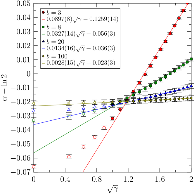
Figure 2: Plot of $\alpha$ as a function of $\sqrt{\gamma}$.

The plot of $C_{0}(b)$ vs $\frac{1}{\sqrt{b}}$ is shown in Fig. 3. The first observation is that the whole range of the plot is less than $0.2\ln(2)$. The second observation is a clear sign that $C_{0}(b)$ tends to zero as $b\to\infty$. The fit of $C_{0}(b)$ to (36), shows that $z_{0}$ is zero within the expected accuracy of this quantity. The other two fits, one with $z_{0}$ forced to zero and the other with $\mu_{0}$ forced to zero, show a larger fluctuation in the non-zero coefficients indicating that we do not have enough data to extract $\mu_{0}$ or $r_{0}$.

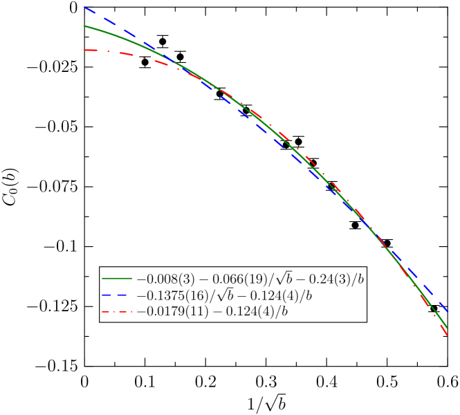
Figure 3: Plot of $C_{0}(b)$ as a function of $b$.

The plot of $C_{1}(b)$ vs $\frac{1}{\sqrt{b}}$ is shown in Fig. 4. A fit to the form in (37) is shown with solid lines. The fit is consistent with $z_{1}=0$ and $\mu_{1}=0$. To further emphasize this point, a fit with $z_{1}$ forced to zero shows that $\mu_{1}$ is still consistent with zero. Finally, a comparison of these two fits to a fit with only the $\frac{1}{b}$ term shows that the coefficient of the non-zero term remains unchanged in the three different cases. Since naïve fermions in two dimensions describe four flavors of fermions, the condensate for a single flavor is estimated as $\frac{\Sigma}{4}=0.34(3)$. This estimate is significantly higher than the analytical result [10] but this is to be expected since we only used $\gamma>1$ in our fits.

Figure 4: Plot of $C_{1}(b)$ as a function of $b$.

5 Discussion

The analysis in section 3 shows that the absence of a critical chemical potential in two dimensional large $N$ gauge theory can be seen at the tree level. Numerical analysis presented in section 4 supports the tree level argument. The basic result is that the critical chemical potential behaves as $(\ln 2)\sqrt{b}$ for naïve fermions and one can extract the coefficient of the $\sqrt{b}$ term using a tree level calculation. The coefficient of the $\sqrt{b}$ term (equivalently, the constant term in (34)) will depend on the fermion discretization but one can show on general grounds that this coefficient is positive for any discretization. The doubly periodic function, $f(u,v)$, in (29) is the naïve fermion determinant on a single site lattice in the presence of a $U(1)$ gauge field of the form $\left(e^{iu},e^{iv}\right)$ and is a positive function for all $(u,v)$. Different fermion discretizations will lead to different expressions for $f(u,v)$ but they will all have the general property that it is a positive function for all $(u,v)$. It follows that

$$\bar{f}(0,0)>\bar{f}(n,m)\ \ \ \ \ \ \ \ \forall(n,m)\neq(0,0)$$ (38)

in (39). Since $\bar{f}(n,m)$ are raised to the $N$th power upon integration over the gauge fields in (27) as a consequence of the identity in Appendix A, it follows that $\bar{f}^{N}(0,0)$ will dominate in the large $N$ limit resulting in a positive constant term in (34) and there by driving the critical chemical potential to infinity.

The above argument shows that there is no critical chemical potential for quarks in two dimensional large $N$ QCD. If Eguchi-Kawai reduction is not valid, as is the case in $d>2$, then we cannot work on a finite lattice in the continuum limit and the arguments in this paper do not hold.

Two dimensional QCD has also been studied in the Hamiltonian formalism [11, 12]. Baryons have been discussed in the Hartree-Fock approximation [11] and the role of chemical potential and temperature have also been discussed [12]. Contrary to the Euclidean Lagrangian formalism where reduction makes the independence on temperature quite obvious, it is harder to see the same result in the Hamiltonian formalism [12]. Arguments in support of the existence of a critical chemical potential is provided in [12] along with the possible breakdown of translational invariance at high densities. The dependence on spatial momentum is suppressed in our analysis since $M$ dominates the denominator of the integrand in (20). This can also be seen in the expression for the critical chemical potential in (23) and this is a consequence of the integration over the Polyakov loop variables defined in (27). The Hamiltonian formalism, by construction, is in the continuum time limit and starts with the theory in the Weyl (temporal) gauge ($A_{0}=0$) and imposes periodic boundary conditions on the spatial gauge field in the time direction. This amounts to setting the Polyakov loop in the time direction to unity which is not consistent with the unbroken $Z_{N}$ symmetry. Recently, the importance of the role of Polyakov loop variables in the spatial direction has been addressed in the Hamiltonian formalism [13].

Appendix A A useful integral

Let $f(u,v)$ be a periodic function of $u$ and $v$ with period $2\pi$. We decompose it into its fourier components according to

$$f(u,v)=\sum_{n=-\infty}^{\infty}\sum_{m=-\infty}^{\infty}\bar{f}(n,m)e^{i\left(nu+mv\right)}.$$ (39)

Then, the integral

$$I_{N}(p,q)=\int\prod_{i=1}^{N}\frac{du_{i}}{2\pi}\prod_{i=1}^{N}\frac{dv_{i}}{2\pi}\prod_{i=1}^{N}f\left(u_{i}+p,v_{i}+q\right)2\pi\delta\left(\sum_{i=1}^{N}u_{i}\right)2\pi\delta\left(\sum_{i=1}^{N}v_{i}\right)$$ (40)

is

$$I_{N}(p,q) = \sum_{n_{i}=-\infty}^{\infty}\sum_{m_{i}=-\infty}^{\infty}\left[\prod_{i=1}^{N}\bar{f}(n_{i},m_{i})\right]$$ (42)

$$\ \ \ \int\prod_{i=1}^{N}\frac{du_{i}}{2\pi}\int\prod_{i=1}^{N}\frac{dv_{i}}{2\pi}e^{i\sum_{i=1}^{N}n_{i}\left(u_{i}+p\right)+m_{i}\left(v_{i}+q\right)}2\pi\delta\left(\sum_{i=1}^{N}u_{i}\right)2\pi\delta\left(\sum_{i=1}^{N}v_{i}\right)$$

$$= \sum_{n=-\infty}^{\infty}\sum_{m=-\infty}^{\infty}\bar{f}^{N}(n,m)e^{iN\left(np+mq\right)}.$$ (43)

References

- [1] G. ’t Hooft, Nucl. Phys. B 75, 461 (1974).
- [2] A. A. Migdal, Sov. Phys. JETP 42, 413 (1975) [Zh. Eksp. Teor. Fiz. 69, 810 (1975)].
- [3] B. E. Rusakov, Mod. Phys. Lett. A 5, 693 (1990).
- [4] T. Eguchi and H. Kawai, Phys. Rev. Lett. 48, 1063 (1982).
- [5] G. Bhanot, U. M. Heller and H. Neuberger, Phys. Lett. B 113, 47 (1982).
- [6] G. ’t Hooft, Nucl. Phys. B 72, 461 (1974).
- [7] D. J. Gross and E. Witten, Phys. Rev. D 21, 446 (1980).
- [8] M. P. Lombardo, PoS C POD2006, 003 (2006) [arXiv:hep-lat/0612017].
- [9] D. J. Gross and Y. Kitazawa, Nucl. Phys. B 206, 440 (1982).
- [10] J. Kiskis, R. Narayanan and H. Neuberger, Phys. Rev. D 66, 025019 (2002) [arXiv:hep-lat/0203005].
- [11] L. L. Salcedo, S. Levit and J. W. Negele, Nucl. Phys. B 361, 585 (1991).
- [12] V. Schon and M. Thies, arXiv:hep-th/0008175.
- [13] B. Bringoltz, arXiv:0811.4141 [hep-lat].