Shattering and coagulation of dust grains in interstellar turbulence

Abstract

We investigate shattering and coagulation of dust grains in turbulent interstellar medium (ISM). The typical velocity of dust grain as a function of grain size has been calculated for various ISM phases based on a theory of grain dynamics in compressible magnetohydrodynamic turbulence. In this paper, we develop a scheme of grain shattering and coagulation and apply it to turbulent ISM by using the grain velocities predicted by the above turbulence theory. Since large grains tend to acquire large velocity dispersions as shown by earlier studies, large grains tend to be shattered. Large shattering effects are indeed seen in warm ionized medium (WIM) within a few Myr for grains with radius $a\ga 10^{-6}$ cm. We also show that shattering in warm neutral medium (WNM) can limit the largest grain size in ISM ($a\sim 2\times 10^{-5}~{}\mathrm{cm}$). On the other hand, coagulation tends to modify small grains since it only occurs when the grain velocity is small enough. Coagulation significantly modifies the grain size distribution in dense clouds (DC), where a large fraction of the grains with $a<10^{-6}$ cm coagulate in 10 Myr. In fact, the correlation among $R_{V}$, the carbon bump strength, and the ultraviolet slope in the observed Milky Way extinction curves can be explained by the coagulation in DC. It is possible that the grain size distribution in the Milky Way is determined by a combination of all the above effects of shattering and coagulation. Considering that shattering and coagulation in turbulence are effective if dust-to-gas ratio is typically more than $\sim 1/10$ of the Galactic value, the regulation mechanism of grain size distribution should be different between metal-poor and metal-rich environments.

1 Introduction

Dust grains absorb stellar ultraviolet (UV)–optical light and reprocess it into far-infrared (FIR), thereby affecting the energetics of interstellar medium (ISM) (e.g. Hirashita & Ferrara, 2002). For this process concerning the interaction between grains and radiation, the optical properties of grains are important. The grain optical properties are determined not only by dust species but also by the grain size (e.g. Draine & Lee, 1984). In fact, the grain species and size distribution are derived from the observed interstellar extinction curve (Mathis et al., 1977, hereafter MRN). These grain properties also affect the FIR spectrum of dust emission (e.g. Takeuchi et al., 2005).

The grain size distribution is known to be affected by various processes in the interstellar space. Grains are supplied from stars at their death (Gehrz, 1989) with a certain grain size distribution (Dominik, Gail, & Sedlmayr, 1989; Todini & Ferrara, 2001; Nozawa et al., 2003; Bianchi & Schneider, 2007; Nozawa et al., 2007). These grains dispersed from stars are processed in the interstellar space. They grow in dense environments such as molecular clouds by grain-grain coagulation (Chokshi, Tielens, & Hollenbach, 1993) and accretion of heavy elements (Spitzer, 1978). They are also destroyed by supernova shocks by gas-grain sputtering and by grain-grain collision (shattering) (Dwek & Scalo, 1980; Tielens et al., 1994; Borkowski & Dwek, 1995). In particular, Jones, Tielens, & Hollenbach (1996, hereafter JTH96) show that the grain size distribution can be significantly modified by shattering. Such a change of grain size distribution would significantly modify the extinction curve and the infrared spectral energy distribution of dust emission.

Potential importance of shattering and coagulation in ISM has often been pointed out, since relative velocity between grains is naturally expected if ISM is turbulent (Kusaka et al., 1970; Völk et al., 1980; Draine, 1985; Ossenkopf, 1993; Lazarian & Yan, 2002). Because turbulence is ubiquitous in ISM (e.g. McKee & Ostriker, 2007), the relative grain motion induced by turbulence is of general importance in the grain evolution in ISM. Moreover, the ISM is known to be magnetized (Arons & Max, 1975). Thus, dust motion in magnetohydrodynamic (MHD) turbulence should be considered. Yan et al. (2004, hereafter YLD04) calculate the relative grain velocity in compressible MHD turbulence, taking into account gas drag (hydrodrag) and gyroresonance. The basis of their theory can be seen in Lazarian & Yan (2002) and Yan & Lazarian (2003). According to their results, grains can be accelerated to a velocity larger than a few km s^-1 in diffuse medium by gyroresonance. At such a high velocity, grains can be shattered (JTH96). On the other hand, small grains can obtain velocities small enough for coagulation to occur, especially in dense medium (YLD04).

The size distribution of grains processed in various ISM phases was investigated by O’Donnell & Mathis (1997). Their models incorporate coagulation by turbulent motion in clouds, accretion of gas-phase metals onto grains, and shattering and sputtering in interstellar shocks. They also take into account the phase exchange of the ISM. They show that both the observed extinction curve and the observed depletion of refractory elements are reproduced by considering phase exchange among diffuse clouds, warm neutral intercloud gas, and molecular clouds. In their models, shattering mainly occurs in ISM shocks. However, Yan & Lazarian (2003) shows that grains can be accelerated to velocities large enough for shattering in MHD turbulence. Thus, it is worth focusing on the effect of turbulence on the grain size distribution. In addition, the treatment of shattering can be revised by including the framework of JTH96 to take into account the velocity dependence of fragment production. It is also useful to compare the difference between the size distribution modified by supernova shocks as treated by JTH96 and that by interstellar turbulence as examined in this paper.

The aim of this paper is to examine quantitatively whether or not shattering and coagulation in turbulent ISM really modify the grain size distribution. We focus on the effects of MHD turbulence as treated in Yan & Lazarian (2003). The other types of dust processing such as shattering and sputtering in supernova shocks and dust condensation in stellar mass loss are not treated in this paper, in order to make our discussions concentrated and clear. For an observational comparison, we adopt the Milky Way extinction curve following O’Donnell & Mathis (1997).

This paper is organized as follows. First, in Section 2, we describe the model adopted to treat shattering and coagulation in turbulent ISM. Then, in Section 3, we overview the results. In Section 4, we discuss our results, focusing on the regulation mechanism of the grain size distribution in turbulent ISM. Section 5 is devoted to the summary.

2 Model

We consider the evolution of grain size distribution by shattering and coagulation induced by relative grain motions in turbulence. In our models, shattering and coagulation are treated simultaneously. The basic ingredients for shattering and coagulation are taken from JTH96 and Chokshi et al. (1993), respectively. We do not consider vaporization in grain collision, since this process does not change the grain size significantly at velocities (at most a few tens km s^-1) achieved in turbulence. Our results are most sensitive to the collision rate between grains. Thus, first of all, the grain velocities adopted are discussed. Then, the frameworks of shattering and coagulation are explained.

2.1 Grain motion

We assume spherical grains (Section 2.2). The velocity of a grain with radius $a$ in the presence of interstellar MHD turbulence is taken from YLD04, who calculated the grain velocities achieved in various phases of ISM (CNM, WNM, WIM, MC, and DC, which stand for cold neutral medium, warm neutral medium, warm ionized medium, molecular cloud, dense cloud, respectively). The physical parameters which they adopted for each phase are listed in Table 1. For DC, they adopt two different cases for the ionization fraction (DC1 and DC2) to examine the effect of the uncertainty in the cosmic-ray ionization rate. We also adopt the same electrical charge of grains as calculated in YLD04, who considered photoelectric emission and collisions with ions and electrons based on the hydrogen number densities, the electron densities, and the UV radiation fields in Table 1. Since the values adopted for these quantities are those usually assumed for Galactic conditions, we expect that the calculations below are at least reasonable for the Galactic ISM. Grains are accelerated through turbulence hydrodrag and gyroresonance. Below we briefly overview the models of turbulence and gyroresonance adopted by YLD04.

Table 1: The parameters of idealized ISM phases in YLD04. Among them, $T$ is the gas temperature, $n_{\mathrm{H}}$ is the number density of hydrogen atoms, $n_{\mathrm{e}}$ is the number density of electrons, $G_{\mathrm{UV}}$ is the UV intensity relative to the average local interstellar radiation field, $L$ is the injection scale at which equipartition between magnetic and kinetic energies occurs, $V$ is the effective injection velocity at the scale $L$ (i.e. $V=V_{\mathrm{A}}$, where $V_{\mathrm{A}}$ is the Alfvén velocity), and $k_{\mathrm{c}}$ is the wavenumber of the damping scale of turbulence. CNM: cold neutral medium; WNM: warm neutral medium; WIM: warm ionized medium; MC: molecular cloud; DC: dark cloud.

ISM Phase	CNM	WNM	WIM	MC	DC1	DC2
$T$ (K)	100	6000	8000	25	10
$n_{\mathrm{H}}$ (cm-3)	30	0.3	0.1	300	$10^{4}$
$n_{\mathrm{e}}$ (cm-3)	0.03	0.03	0.0991	0.03	0.01	0.001
$G_{\mathrm{UV}}$	1	1	1	0.1	0.01	0.001
$B$ ($\mu$G)	6	5.8	3.35	11	80
$L$ (pc)	0.64	100	100	1	1
$V=V_{\mathrm{A}}$ (km s-1)	2	20	20	1.2	1.5
$k_{\mathrm{c}}$ (cm-1)	$7\times 10^{-15}$	$4\times 10^{-17}$	—	$4.5\times 10^{-14}$	$5.3\times 10^{-15}$	$5.3\times 10^{-17}$

2.1.1 Turbulence

The velocity achieved by hydrodrag is determined by the largest scale on which grains are decoupled from the hydrodynamical motion, since the turbulent velocity is larger on larger scales. Thus, larger grains, which tend to be coupled with larger-scale motions, are more accelerated. In general, neutral medium tends to accelerate grains less than ionized medium because of ion-neutral collision damping of MHD turbulence. For example, the grain velocity in DC2 is smaller than DC1 because of the difference in ionization degree. The same reason is applied to the larger grain velocities achieved in WIM than in WNM.

YLD04 obtain the scaling relation of turbulence velocity based on a MHD turbulence theory developed by Cho & Lazarian (2002), who decompose MHD fluctuations into Alfvén, slow, and fast modes. Unlike hydrodynamic turbulence, Alfvénic turbulence is anisotropic, with eddies elongated along the magnetic field (Goldreich & Sridhar, 1995). This is because it is easier to mix the magnetic fields lines perpendicular to the direction of the magnetic field rather than to bend them. The energies of eddies drops with the decrease of eddy size, and it becomes more difficult for smaller eddies to bend the magnetic field lines. Therefore, the eddies get more and more anisotropic as the sizes decreases. Eddies mix the magnetic field lines at the rate of $k_{\perp}v_{k}$, where $k_{\perp}$ is a wavenumber measured in the direction perpendicular to the local magnetic field and $v_{k}$ is the mixing velocity. The energy spectrum for the perpendicular motions becomes Kolmogorov-like, i.e. $v_{k}\propto k^{-1/3}$. On the other hand, the magnetic perturbations propagate along the magnetic field lines at the rate $k_{\parallel}V_{\mathrm{A}}$, where $k_{\parallel}$ is the wavenumber parallel to the local magnetic field and $V_{\mathrm{A}}$ is the Alfvén velocity. The mixing motions couple to the wavelike motions parallel to magnetic field, giving a critical balance condition, $k_{\perp}v_{k}\sim k_{\parallel}V_{\mathrm{A}}$. Thus, we obtain $k_{\parallel}\propto k_{\perp}^{2/3}$. The fast modes follow acoustic cascade, and show isotropic energy spectra with $v_{k}\propto k^{-1/4}$ (Cho & Lazarian, 2002).

YLD04 assume that equal amounts of energy are transferred into fast and Alfvén modes when driving is on large scales. The cascades proceed to small scales without much cross talk between those two kinds of modes, according to the results in Cho & Lazarian (2002, 2003). From the scaling relations of $v_{k}$ with $k$, we observe that the decoupling from fast modes usually brings larger velocity dispersions to grains than Alfvén modes.

In this paper, we do not consider imbalanced turbulence, which develops under unequal energy flux from opposite directions and has non-zero cross-helicity. Recent study by Beresnyak & Lazarian (2008) shows that the stronger wave of the Alfvén modes has smaller anisotropy, which indicates that the interaction of the grains with the imbalanced Alfvénic turbulence could be more efficient. However, the results on the imbalanced turbulence is far from quantitative. And there is no conclusive theory yet for the imbalanced fast modes, which are more important for the acceleration according to Yan & Lazarian (2003). The only study so far (Suzuki, Lazarian & Beresnyak, 2007) indicates that fast modes are not so different as in the balanced turbulence. In addition, imbalanced turbulence is applicable to places near an energy source, e.g. the vicinity of a star, which we do not consider in this paper.

The conditions for ISM phases that YLD04 adopt imply that the turbulence is super-Alfvénic ($\delta V\ga V_{\mathrm{A}}$, where $\delta V$ is the turbulence velocity). Indeed given the uncertainty of the strength of the magnetic field in the ISM, we do not know whether the conjecture is universal. However, our results for shattering and coagulation will not be concerned sensitively to the above debate on sub/super-Alfvénic turbulence. The reason is what follows. If the turbulence is sub-Alfvénic, the turbulence is weak. The weak turbulence has only limited inertial range. Moreover, it is the fast modes that dominate the acceleration of dust as demonstrated by Yan & Lazarian (2003). And there has been study showing that fast modes in weak turbulence are similar to fast modes in strong turbulence apart from the modes in the narrow cone around the $\mn@boldsymbol{k}$ vector in Fourier space (Chandran, 2005). When the cascades proceed down to the scale where the critical balance $k_{\bot}v_{k}\sim k_{\|}V_{\mathrm{A}}$ is reached, turbulence becomes strong (Lazarian & Vishniac, 1999). The coherence length of the strong turbulence $LM_{\mathrm{A}}^{2}$, is also the correlation length of the turbulence magnetic field, where $L$ is the injection scale of the turbulence and $M_{\mathrm{A}}\equiv\delta V/V_{\mathrm{A}}$ is the Alfvénic Mach number. It is unlikely that $M_{\mathrm{A}}$ is less than 0.1 in the Galactic environments. Given an injection scale of turbulence at 30 pc, the coherence length of the strong turbulence is then $\ga 0.3$ pc, which is still larger than the Larmor radius of most massive dust ($a=10^{-4}$ cm). In fact, the observations indicate that the correlation length of magnetic field is a few parsecs (Spangler & Minton, 1996).

2.1.2 Gyroresonance

Gyroresonance further accelerates charged grains. Grains obtain energy by resonant interactions with the waves if the resonance condition, $\omega-k_{\parallel}v\mu=n\Omega$ ($n=0,\,\pm 1,\,\pm 2,\,\cdots$), is satisfied, where $\omega$ is the wave frequency, $k_{\parallel}$ is the parallel component of wavevector along the magnetic field, $v$ is the particle velocity, $\mu$ is the cosine of the pitch angle relative to the magnetic field, and $\Omega=qB/(mc)$ is the Larmor frequency of the particle ($q$ is the charge, $B$ is the magnetic field strength, $m$ is the grain mass, and $c$ is the light speed). The above condition indicates that gyroresonance occurs when the Doppler-shifted frequency of the wave in the grain’s guiding centre rest frame is a multiple of the gyrofrequency and when the rotating direction of the electric wavevector is the same as the direction of the Larmor gyration of the grain. Then the steady state distribution function of grains is calculated by a Fokker-Planck equation treating the effects of gyroresonance acceleration and gaseous friction.

Gyroresonance is efficient for large grains: The condition for gyroresonance is that the Larmor frequency $\Omega$ is smaller than the the cutoff wave frequency of the turbulence $\omega_{\mathrm{c}}$. The velocity of accelerated grain only weakly depends on the charge and mass as long as the aforementioned condition is satisfied (YLD04). On the other hand, the energy gain rate of the grains scales linearly with the intensity of MHD turbulence; thus the velocity is roughly proportional to the square root of the intensity of the MHD turbulence.

2.1.3 Overall features of grain velocity

The results in YLD04 indicate that gyroresonance accelerates silicate with $a\ga 2\times 10^{-5}$ cm and graphite with $a\ga 3\times 10^{-5}$ cm to velocities large enough ($\sim 20$ km s^-1) for shattering in WNM. Both silicate and graphite grains with $a\ga\mbox{several}\times 10^{-6}$ cm achieve velocities (1–2 km s^-1) near to the shattering thresholds in CNM (Table 2). Although silicate and graphite with $a\ga 10^{-6}$ cm are accelerated to 20 km s^-1 by gyroresonance in WIM, the acceleration by hydrodrag is larger because the dissipation of turbulence in WIM is less than that in WNM.

Table 2: Summary of grain properties.

Species	$\rho_{\mathrm{gr}}$	$c_{0}$	$s$	$v_{\mathrm{shat}}$	$P_{1}$	$P_{v}$	$\gamma$	$E$	$\nu$
	(g cm-3)	(km s-1)		(km s-1)	(dyn cm-2)	(dyn cm-2)	(erg cm-2)	(dyn cm-2)
Silicate	3.3	5	1.2	2.7	$3\times 10^{11}$	$5.4\times 10^{12}$	25	$5.4\times 10^{11}$	0.17
Graphite	2.2	1.8	1.9	1.2	$4\times 10^{10}$	$5.8\times 10^{12}$	12	$3.4\times 10^{10}$	0.5

On the other hand, low relative velocities of small grains allow coagulation to occur. Moreover, with small velocities, a dense environment is necessary for a high enough collision rate. Thus, coagulation is important in DC for grains with $a\la 10^{-6}$ cm, which have velocities $\la 10^{3}$ cm s^-1. Coagulation is also possible in MC with a smaller rate.

Since YLD04 only calculated the grain velocity for $a\geq 10^{-6}$ cm except for WIM, we extend the calculations down to $a=10^{-7}$ cm. Below $a\sim 10^{-6}$ cm, however, the coupling between gas and grains occurs on a scale smaller than the dissipation scale of turbulence. Thus, the velocities of grains typically smaller than $10^{-6}$ cm are determined by the thermal velocities.

2.2 Time evolution of the grain size distribution

We assume that grains are spherical with a constant material density $\rho_{\mathrm{gr}}$. The mass $m$ and the radius $a$ of a grain are related by

$$m=\frac{4\pi}{3}a^{3}\rho_{\mathrm{gr}}\,.$$ (1)

The number density of grains whose radii are between $a$ and $a+\mathrm{d}a$ is denoted as $n(a)\,\mathrm{d}a$, where the entire range of $a$ is from $a_{\mathrm{min}}$ to $a_{\mathrm{max}}$. The total grain mass is conserved in shattering and coagulation. To ensure the conservation of the total mass of grains, it is numerically convenient to consider the distribution function of grain mass instead of grain size. We denote the number density of grains whose masses are between $m$ and $m+\mathrm{d}m$ as $\tilde{n}(m)\,\mathrm{d}m$. The two distribution functions are related as $n(a)\,\mathrm{d}a=\tilde{n}(m)\,\mathrm{d}m$.

For numerical calculation, we consider $N$ discrete bins for the grain radius. The grain radius in the $i$-th ($i=1,\,\cdots,\,N$) bin is between $a_{i-1}^{\mathrm{(b)}}$ and $a_{i}^{\mathrm{(b)}}$, where $a_{i}^{\mathrm{(b)}}=a_{i-1}^{\mathrm{(b)}}\delta$, $a_{0}^{\mathrm{(b)}}=a_{\mathrm{min}}$, and $a_{N}^{\mathrm{(b)}}=a_{\mathrm{max}}$ (i.e. $\log\delta$ specifies the width of a logarithmic bin: $\log\delta=(1/N)\log(a_{\mathrm{max}}/a_{\mathrm{min}})$). We represent the grain radius and mass in the $i$-th bin with $a_{i}\equiv(a_{i-1}^{\mathrm{(b)}}+a_{i}^{\mathrm{(b)}})/2$ and $m_{i}\equiv(4\pi/3)a_{i}^{3}\rho_{\mathrm{gr}}$. The boundary of the mass bin is defined as $m_{i}^{\mathrm{(b)}}\equiv(4\pi/3)[a_{i}^{\mathrm{(b)}}]^{3}\rho_{\mathrm{gr}}$. Giving $a_{\mathrm{min}}$, $a_{\mathrm{max}}$, and $N$, all bins can be set. A grain in the $i$-th bin is called “grain $i$”. In this paper we take $N=32$ after confirming that the results do not change if we take a larger $N$. For the size range, we assume $a_{\mathrm{min}}=0.001~{}\mu$m and $a_{\mathrm{max}}=0.25~{}\mu$m to reproduce the Milky Way extinction curve (Section 2.4).

The mass density of grains contained in the $i$-th bin, $\tilde{\rho}_{i}$, is defined as

$$\tilde{\rho}_{i}\equiv m_{i}\tilde{n}(m_{i})(m_{i}^{\mathrm{(b)}}-m_{i-1}^{\mathrm{(b)}})\,.$$ (2)

Then, the time evolution of $\tilde{\rho}_{i}$ is expressed as

$$\frac{\mathrm{d}\tilde{\rho}_{i}}{\mathrm{d}t}=\left[\frac{\mathrm{d}\tilde{\rho}_{i}}{\mathrm{d}t}\right]_{\mathrm{shat}}+\left[\frac{\mathrm{d}\tilde{\rho}_{i}}{\mathrm{d}t}\right]_{\mathrm{coag}}\,,$$ (3)

where the first and the second terms in the right-hand side are the contributions from shattering and coagulation, respectively. These two terms are estimated in Sections 2.2.1 and 2.2.2.

We consider silicate and graphite as grain species. In order to avoid complexity in compound species, we only treat collisions between the same species. Although this underestimates the grain collision rate by a factor of $\sim 2$, our simple assumption here is enough to understand the effects of interstellar turbulence on the grain size distribution for the first time. The adopted parameters for each grain species are summarized in Table 2 and are taken from JTH96 and Chokshi et al. (1993). We use the same notation ($n(a)$) for both silicate and graphite size distributions.

2.2.1 Shattering

The time evolution of $\tilde{\rho}_{i}$ by shattering can be written as

$$\left[\frac{\mathrm{d}\tilde{\rho}_{i}}{\mathrm{d}t}\right]_{\mathrm{shat}} = -m_{i}\tilde{\rho}_{i}\sum_{k=1}^{N}\alpha_{ki}\tilde{\rho}_{k}+\sum_{j=1}^{N}\sum_{k=1}^{N}\alpha_{kj}\tilde{\rho}_{k}\tilde{\rho}_{j}m_{\mathrm{shat}}^{kj}(i)\,,$$

$$\alpha_{ki}=\left\{\begin{array}[]{ll}{\displaystyle\frac{\sigma_{ki}v_{ki}}{m_{i}m_{k}}}&\mbox{if $v_{ki}>v_{\mathrm{shat}}$,}\\ 0&\mbox{otherwise,}\end{array}\right.$$ (7)

where $m_{\mathrm{shat}}^{kj}(i)$ is the total mass of the shattered fragments of a grain $k$ that enter the $i$-th bin in the collision between grains $k$ and $j$, $\sigma_{ki}$ and $v_{ki}$ are, respectively, the grain-grain collisional cross section and the relative collision speed between grains $k$ and $i$, and $v_{\mathrm{shat}}$ is the velocity threshold for shattering to occur. For the cross section, we apply $\sigma_{ki}=\pi(a_{k}+a_{i})^{2}$.

The grain velocities given by YLD04 are typical velocity dispersions. The relative velocity $v_{ki}$ is treated with a similar manner to Appendix A of JTH96. Each time step is divided into 4 small steps, and we apply $v_{ik}=v_{i}+v_{k}$, $|v_{i}-v_{k}|$, $v_{i}$, and $v_{k}$ in each small step, where $v_{i}$ and $v_{k}$ are the velocities of grains $i$ and $k$, respectively (see Section 2.1). Note that the mass distribution of the shattered fragment $m_{\mathrm{shat}}^{kj}(i)$ depends on $v_{kj}$. The method for calculating $m_{\mathrm{shat}}^{kj}(i)$ is described in Section 2.3.

2.2.2 Coagulation

The time evolution of $\tilde{\rho}_{i}$ by coagulation can be written in a similar form to equation (LABEL:eq:time_ev):

$$\left[\frac{\mathrm{d}\tilde{\rho}_{i}}{\mathrm{d}t}\right]_{\mathrm{coag}} = -m_{i}\tilde{\rho}_{i}\sum_{k=1}^{N}\alpha_{ki}\tilde{\rho}_{k}+\sum_{j=1}^{N}\sum_{k=1}^{N}\alpha_{kj}\tilde{\rho}_{k}\tilde{\rho}_{j}m_{\mathrm{coag}}^{kj}(i)\,,$$

$$\alpha_{ki}=\left\{\begin{array}[]{ll}{\displaystyle\frac{\sigma_{ki}v_{ki}}{m_{i}m_{k}}}&\mbox{if $v_{ki}<v_{\mathrm{coag}}^{ki}$,}\\ 0&\mbox{otherwise.}\end{array}\right.$$ (11)

Here, $m_{\mathrm{coag}}^{kj}(i)=m_{i}$ if $m_{i-1}^{\mathrm{(b)}}\leq m_{k}+m_{j}<m_{i}^{\mathrm{(b)}}$; otherwise $m_{\mathrm{coag}}^{kj}(i)=0$. The coagulation is assumed to occur only if the relative velocity is less than the coagulation threshold velocity $v_{\mathrm{coag}}^{ki}$. The coagulation threshold velocity is given by (Chokshi et al. 1993; Dominik & Tielens 1997; YLD04)

$$v_{\mathrm{coag}}^{ki}=2.14F_{\mathrm{stick}}\left[\frac{a_{k}^{3}+a_{i}^{3}}{(a_{k}+a_{i})^{3}}\right]^{1/2}\frac{\gamma^{5/6}}{E^{1/3}R_{ki}^{5/6}\rho_{\mathrm{gr}}^{1/2}}\,,$$ (12)

where a factor $F_{\mathrm{stick}}=10$ is introduced following YLD04 (based on the experimental work by Blum 2000), $\gamma$ is the surface energy per unit area, $R_{ki}\equiv a_{k}a_{i}/(a_{k}+a_{i})$ is the reduced radius of the grains, $E$ is related to Poisson’s ratios ($\nu_{k}$ and $\nu_{i}$) and Young’s modulus ($E_{k}$ and $E_{i}$) by $1/E\equiv(1-\nu_{k})^{2}/E_{k}+(1-\nu_{i})^{2}/E_{i}$. The values of $\gamma$ and $E$ are taken from Table 3 of Chokshi et al. (1993) (the data for quartz and graphite are used for silicate and graphite, respectively) as summarized in Table 2. The treatment of $v_{ki}$ in coagulation is the same as that in shattering (Section 2.2.1).

Although the above form of coagulation threshold velocity is derived based on both physical and experimental basis, there could be significant uncertainties. A change of the coagulation threshold affects the largest size of grains subject to coagulation, since larger grains have larger velocities. For example, as shown later, the coagulation condition is satisfied for grains with $a\la\mbox{a few}\times 10^{-6}$ cm. However, we have confirmed that even if the coagulation threshold is altered by a factor of ten from the above values, the size of grains subject to coagulation changes only by a factor of 2–3. This is because of a steep dependence of the grain velocity on the grain size.

2.3 Production of shattered fragments

Here we determine the mass distribution of the shattered fragments, $m_{\mathrm{shat}}^{kj}(i)$, in equation (LABEL:eq:time_ev). The shattering rate is determined mostly by the collision frequency between grains. Thus, the overall results in this paper is less sensitive to the detailed model of shattered fragments than to the grain velocities. Indeed, JTH96 show that the size distribution of shattered fragments does not have a large influence on the overall grain size distribution. We have also confirmed that the specific parameters adopted in this subsection do not affect the results significantly. We can have an idea about the uncertainties caused by the material parameters by comparing the results for silicate and graphite. Since the results in these two materials are broadly similar, the assumption on the material parameters only has a secondary importance in our models as long as there are not very eccentric materials involved.

We illustrate our treatment of shattering in Fig. 1. We consider a collision between grains $k$ and $j$ (here we assume $k\geq j$), and call the grains labeled as $k$ and $j$ target and projectile, respectively. The necessary material quantities are summarized in Table 2. The mass shocked to the critical pressure for cratering in the target, $M$, is given by (Tielens et al. 1994; JTH96)

$$\frac{M}{m_{j}}=\frac{1+2{\cal R}}{(1+{\cal R})^{9/16}}\frac{1}{\sigma_{r}^{1/9}}\left(\frac{{\cal M}_{r}^{2}}{\sigma_{1}{\cal M}_{1}^{2}}\right)^{8/9}\,,$$ (13)

where ${\cal R}=1$ in the collision between the same species (we adopt ${\cal R}=1$ in this paper), ${\cal M}_{r}\equiv v_{kj}/c_{0}$ ($c_{0}$ is the sound speed of the grain material), $\sigma_{1}$ and $\sigma_{1i}$ are constants typically of order unity (equation 15), and ${\cal M}_{1}$ is the Mach number corresponding to the critical pressure $P_{1}$:

$${\cal M}_{1}=\frac{2\phi_{1}}{1+(1+4{s}\phi_{1})^{1/2}}\,,$$ (14)

where $\phi_{1}\equiv P_{1}/(\rho_{\mathrm{gr}}c_{0}^{2})$, and ${s}$ is a dimensionless material constant that determines the relation between the shock velocity and the velocity of the shocked matter. Using the following expression for $\sigma$ as

$$\sigma({\cal M})\equiv\frac{0.30({s}+{\cal M}^{-1}-0.11)^{0.13}}{{s}+{\cal M}^{-1}-1}\,,$$ (15)

we obtain $\sigma_{1}=\sigma({\cal M}_{1})$ and $\sigma_{1i}=\sigma({\cal M}_{r}/(1+{\cal R}))$. We assume that if more than the half of the target is shocked (i.e. $M>m_{k}/2$) the entire target is shattered (i.e. $m_{\mathrm{frag}}=m_{k}$ in equation 17, where $m_{\mathrm{frag}}$ is the total mass of the fragments). Otherwise, only a fraction of the target mass ($M_{\mathrm{ej}}$) is ejected from the target (i.e. $m_{\mathrm{frag}}=M_{\mathrm{ej}}$). $M_{\mathrm{ej}}$ is assumed to be $0.40M$, i.e. 40% of the shocked mass is finally ejected. This fraction is derived for $z=3.4$, where the radial velocity of the cratering flow in the shattered material is approximated to be $\propto R^{-z}$ ($R$ is the distance from the cratering centre; JTH96). Finally, the entire projectile is assumed to fragment into small pieces (i.e. $m_{\mathrm{frag}}=m_{j}$ for all projectiles).

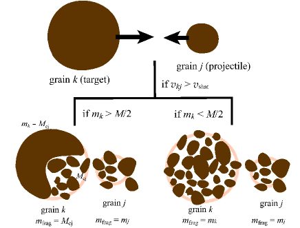
Figure 1: Schematic figure of our treatment of shattering. We consider a collision of two grains in the $k$-th size bin and the $j$-th size bin (called grain $k$ and grain $j$, respectively) with a relative velocity of $v_{kj}$. We call the larger and smaller grains “target” and “projectile”, respectively. Here we assume $k\geq j$; that is, the target is grain $k$ and the projectile is grain $j$. If the shocked mass $M$ in the target is larger than the mass of the target $m_{k}$ ($M>m_{k}/2$), we assume that the entire target fragments into small pieces ($m_{\mathrm{frag}}=m_{k}$). If $M<m_{k}/2$, a part of the target mass, $M_{\mathrm{ej}}$ is shattered and ejected ($m_{\mathrm{frag}}=M_{\mathrm{ej}}$). The entire projectile is assumed to fragment ($m_{\mathrm{frag}}=m_{j}$). The size distribution of the fragments is assumed to follow equation (16).

The fragments are assumed to follow the size distribution (Hellyer 1970; JTH96)

$$n_{\mathrm{frag}}(a)\,\mathrm{d}a=C_{\mathrm{frag}}a^{-3.3}\,\mathrm{d}a\,,$$ (16)

where the normalization constant $C_{\mathrm{frag}}$ is determined by

$$m_{\mathrm{frag}}=\int_{a_{\mathrm{fmin}}}^{a_{\mathrm{fmax}}}mn_{\mathrm{frag}}(a)\,\mathrm{d}a\,.$$ (17)

Here, $a_{\mathrm{fmin}}$ and $a_{\mathrm{fmax}}$, respectively, specify the upper and lower bounds of the fragment radius, which are determined in Sections 2.3.1 and 2.3.2 for the projectile and the target, respectively. If $a_{\mathrm{fmin}}$ estimated is less than $a_{\mathrm{min}}$, we take $a_{\mathrm{fmin}}=a_{\mathrm{min}}$. If $a_{\mathrm{fmax}}$ is also smaller than $a_{\mathrm{min}}$, all the fragments are put in the bin with the smallest size (i.e. $i=0$). Finally, the mass of shattered fragments in the $i$-th bin is determined in terms of $n_{\mathrm{frag}}$ as

$$m_{\mathrm{shat}}(i)=\int_{a_{i-1}^{\mathrm{(b)}}}^{a_{i}^{\mathrm{(b)}}}mn_{\mathrm{frag}}(a)\,\mathrm{d}a\,,$$ (18)

where the integration is performed in the range corresponding to the $i$-th bin. We put this mass in equation (LABEL:eq:time_ev) (note that the superscript $kj$ is omitted here).

In the following, we summarize how to determine $a_{\mathrm{fmin}}$ and $a_{\mathrm{fmax}}$.

2.3.1 Projectile $m_{j}$

The entire projectile is assumed to fragment into small pieces, i.e. $m_{\mathrm{frag}}=m_{j}$. The maximum grain size, $a_{\mathrm{fmax}}$, is determined by (JTH96)

$$a_{\mathrm{fmax}}=0.22a_{j}\left(\frac{v_{\mathrm{cat}}}{v_{kj}}\right)\,,$$ (19)

where $v_{\mathrm{cat}}$ is the critical spalling collision velocity given by

$$v_{\mathrm{cat}}=c_{0}\left[\frac{m_{k}}{(1+2{\cal R})m_{j}}\right]^{9/16}\sigma_{1}^{1/2}\sigma_{1i}^{1/16}(1+{\cal R}){\cal M}_{1}\,.$$ (20)

The minimum grain size, $a_{\mathrm{fmin}}$, is determined by

$$a_{\mathrm{fmin}}=0.03a_{\mathrm{fmax}}\,.$$ (21)

2.3.2 Target $m_{k}$

If $M/m_{k}>0.5$, we assume that the entire target fragments into small pieces; i.e. $m_{\mathrm{frag}}=m_{k}$. The maximum and minimum fragment sizes are determined by equations (19) and (21), respectively, but $j$ and $k$ are exchanged.

If $M/m_{k}\leq 0.5$, we assume that the mass $M_{\mathrm{ej}}$ ($=0.40M$) fragments into smaller grains (i.e. $m_{\mathrm{frag}}=M_{\mathrm{ej}}$), and a grain with mass of $m_{k}-M_{\mathrm{ej}}$ is left, which is put in the corresponding bin. According to equations (10) and (15) in JTH96, the largest fragment size and the total ejected volume ($M_{\mathrm{ej}}/\rho_{\mathrm{gr}}$) can be related by

$$M_{\mathrm{ej}}/\rho_{\mathrm{gr}}=\frac{16}{3}\pi\frac{z^{3}(z-2)}{z+1}a_{\mathrm{fmax}}^{3}\,.$$ (22)

We determine $a_{\mathrm{fmax}}$ according to this equation with $z=3.4$. The following estimate is adopted for $a_{\mathrm{fmin}}$ (JTH96):

$$a_{\mathrm{fmin}}=a_{\mathrm{fmax}}\left(\frac{P_{1}}{P_{v}}\right)^{1.47}\,,$$ (23)

where $P_{v}$ is the critical pressure for vaporization (Table 2).

2.4 Initial Grain Size Distribution

It is not an easy task to select a good initial grain size distribution, since the grain production in stellar mass loss is not fully understood yet. Thus, we concentrate on how the standard grain size distribution is modified by shattering and coagulation in various ISM phases. As the standard grain size distribution, we adopt

$$n(a)={\cal C}a^{-K}~{}(a_{\mathrm{min}}\leq a\leq a_{\mathrm{max}})\,,$$ (24)

where ${\cal C}$ is the normalizing constant. We select $K=3.5$ as derived by MRN to explain the observed Milky Way extinction curve. For the size range, we assume $a_{\mathrm{min}}=0.001~{}\mu$m and $a_{\mathrm{max}}=0.25~{}\mu$m for both graphite and silicate (MRN; Li & Draine 2001), although Li & Draine (2001) adopt more elaborate functional form (see also Kim, Martin, & Hendry 1994). In fact, as shown later, the predicted extinction curve is broadly consistent with the observed extinction curve (Section 3.2). Thus, the above simple assumption for the size distribution is enough for our purpose.

The normalization factor ${\cal C}$ is determined according to the mass density of the grains in the ISM:

$${\cal R}m_{\mathrm{H}}n_{\mathrm{H}}=\int_{a_{\mathrm{min}}}^{a_{\mathrm{max}}}\frac{4\pi}{3}a^{3}\rho_{\mathrm{gr}}{\cal C}a^{-K}\,\mathrm{d}a\,,$$ (25)

where $n_{\mathrm{H}}$ is the hydrogen number density given for each ISM phase in YLD04 (see also Table 1), $m_{\mathrm{H}}$ is the hydrogen atom mass, and ${\cal R}$ is the dust-to-hydrogen mass ratio (i.e. dust abundance relative to hydrogen) in the ISM. We adopt ${\cal R}=4.0\times 10^{-3}$ and $3.4\times 10^{-3}$ for silicate and graphite, respectively (, 2003). As shown in Section 3.2, the size distribution assumed here reproduces the observed Milky Way extinction curve.

2.5 Timescales

We calculate the change of grain size distribution in various ISM phases on typical timescales. The typical timescale of the phase change among WIM, WNM, and CNM is $\sim\mbox{a few}\times 10^{7}$–$10^{8}$ yr (Ikeuchi, 1988; O’Donnell & Mathis, 1997; Hirashita & Kamaya, 2001). For WIM, there is another relevant timescale, that is, recombination timescale. With hydrogen number density $\sim 0.1$ cm^-3 and temperature $\sim 10^{4}$ K, the recombination timescale is roughly $\sim 10^{6}$ yr (Spitzer, 1978). As shown later, the grains are shattered too much in WIM for a time $t\ga 10^{7}$ yr, so a timescale of the order of Myr is more appropriate for WIM (Section 3). For denser medium, a short lifetime may be reasonable, and indeed the lifetime of molecular clouds is estimated to be $\sim 10^{7}$ yr (Blitz & Shu, 1980; Palla & Stahler, 2002; Kawamura et al., 2007) or shorter (Elmegreen, 2000; Hartmann, 2003). Thus, we examine $t<10^{7}$ yr for MC and DC. These timescales are also consistent with O’Donnell & Mathis (1997).

2.6 Extinction curves

Following O’Donnell & Mathis (1997), we use extinction curves to test our results. We calculate extinction curves by using the optical constants of astronomical silicate and graphite taken from Draine & Lee (1984). Then cross sections for absorption and scattering are calculated with Mie theory (Bohren & Huffman, 1983) and weighted for the grain size distribution. Finally the extinction curves of silicate and graphite are summed up. The extinction is normalized to the number density of hydrogen atoms.

For comparison, the observational data of the standard interstellar extinction of the Milky Way is taken from Pei (1992). Bohlin, Savage, & Drake (1978) show that the mean Milky Way $N_{\mathrm{H}}/E(B-V)$ ($N_{\mathrm{H}}$ is the column density of hydrogen atoms and $E(B-V)$ is the excess of $B-V$ colour) is $5.8\times 10^{21}$ atoms cm^-2 mag^-1. Then by using $A_{B}=(1+R_{V})E(B-V)$ ($A_{\lambda}$ is the extinction in units of magnitude at wavelength $\lambda$ and $R_{V}\equiv A_{V}/E(B-V)$), and adopting $R_{V}=3.08$ (Pei, 1992), we obtain $N_{\mathrm{H}}/A_{B}=1.422\times 10^{21}$ atoms cm^-2 mag^-1 for the mean Milky Way extinction. Pei (1992) lists $\xi(\lambda)\equiv A_{\lambda}/A_{B}$ for relevant wavelengths, and the equation $A_{\lambda}/N_{\mathrm{H}}=\xi(\lambda)A_{B}/N_{\mathrm{H}}$ can be used to obtain $A_{\lambda}/N_{\mathrm{H}}$ for the mean Milky Way extinction curve. The extinction curves are often normalized to the value at $V$ band, but we do not adopt this normalization, because the $V$ band extinctions themselves in our models are significantly affected by a slight change of the size distribution at $10^{-6}~{}\mathrm{cm}<a<10^{-5}~{}\mathrm{cm}$ (Section 3). Since our models are based on a simple analytical treatment of interstellar turbulence with a single density, it is not reasonable to adopt a normalization parameter which is not robust to the change of details in the models.

It is also known that there is a variation in the Milky Way extinction curves along various lines of sight. Cardelli, Clayton, & Mathis (Cardelli et al.1989) argue that the variation of the extinction curves can be parametrized by $R_{V}$. More recently, Fitzpatrick & Massa (2007) show that the variance of the extinction curves normalized to $A_{V}$ is roughly 20% at $1/\lambda=8~{}\mu\mathrm{m}^{-1}$ and roughly 10% at the 2175Å bump. Although we do not adopt the normalization at $V$ band in the extinction curve, these variances provide us with a rough idea as to how much variation of the extinction curve is permitted in the Galactic environment.

3 Results

3.1 Grain size distribution

In Figs. 2 and 3, we show the size distributions of silicate and graphite, respectively, for various ISM phases. The size distribution is expressed by multiplying $a^{4}$ to show the “mass distribution” in each logarithmic bin of the grain size (O’Donnell & Mathis, 1997); i.e. $a^{3}$ comes from the grain mass and another factor $a$ originates from $\mathrm{d}a/\mathrm{d}\ln a=a$. The largest change is seen in WIM, for which we present the grain size distributions in the shortest timescales (1 Myr and 5 Myr). If the grains are processed for a longer time in WIM, the extinction curves become too modified to be consistent with the observed Milky Way extinction curve (Section 3.2). In WIM, grains with $a\ga\mbox{a few}\times 10^{-6}$ cm are efficiently accelerated by up to a velocity larger than the shattering threshold velocity. If the grain velocity is the same, shattering efficiently destroys small grains because of their large surface-to-volume ratios. Thus, the largest shattering efficiency is realized for the smallest grains which obtain a velocity above the shattering threshold. For this reason, grains with $a\sim 10^{-6}$ cm are the most efficiently shattered in WIM. This is different from shattering in supernova shocks, where such small grains are not efficiently shattered (JTH96) since small grains tend to be decelerated quickly by the gas drag.

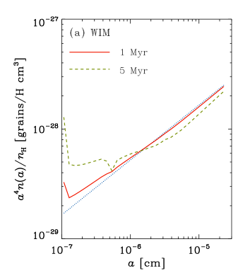
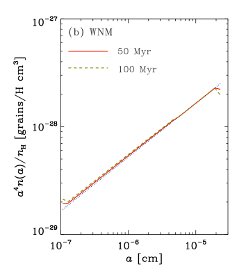
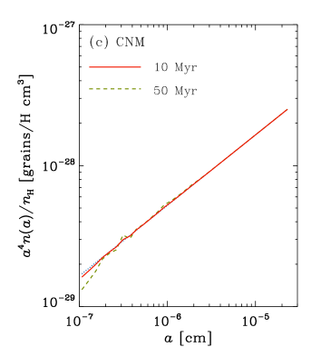
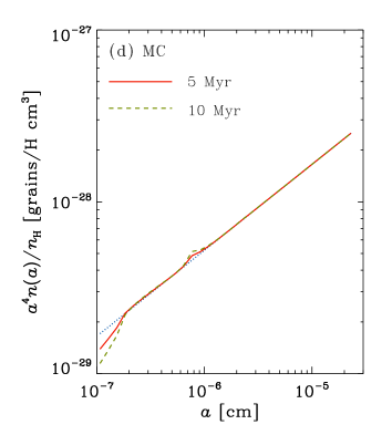
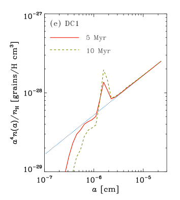
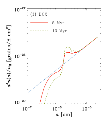
Figure 2: The grain size distributions for silicate in (a) WIM, (b) WNM, (c) CNM, (d) MC, (e) DC1, and (f) DC2. The initial MRN distribution is shown by the dotted line. The solid (dashed) line presents the distribution at $t=1$ Myr ($t=5$ Myr) for Panel (a), $t=10$ Myr and 50 Myr for Panels (b) and (c), and at $t=5$ Myr ($t=10$ Myr) for Panels (d), (e), and (f). In this paper, the grain size distributions are presented by multiplying $a^{4}$ to show the mass distribution in each logarithmic bin of the grain radius. The grain size distribution is normalized to the hydrogen number density $n_{\mathrm{H}}$.

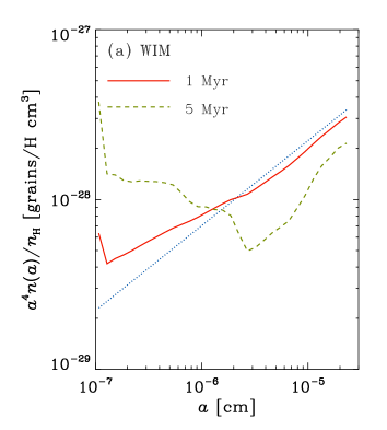
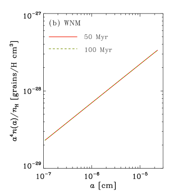
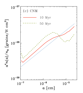
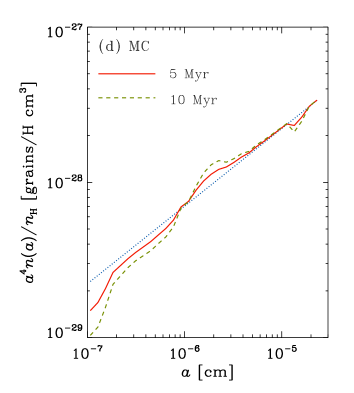
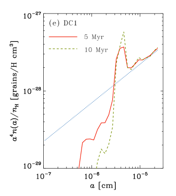
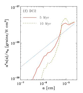
Figure 3: Same as Fig. 2 but for graphite.

In WNM, because of the ion-neutral collision, the fast modes are damped on a larger scale than in WIM. Thus, gyroresonance is not efficient for small grains, and only large grains with $a>0.2~{}\mu$m for silicate and with $a>0.3~{}\mu$m for graphite can be accelerated to a velocity large enough for shattering. (Note that graphite grains are not shattered since we only consider $a\leq 0.25~{}\mu$m.) Those threshold radii for gyroresonance are quite robust because they only weakly depend on the charge, the magnetic field strength, and the grain density as mentioned in Section 2.1.2. It is interesting that those grain sizes satisfying the shattering condition in WNM are nearly the upper grain size in the Milky Way (MRN). Thus, the upper limit of the grain size is possibly determined by shattering in WNM. This issue is further investigated in Section 4.2.

Shattering takes place also in CNM for graphite because graphite has lower shattering threshold velocity than silicate. However, the result is sensitive to slight changes in the shattering threshold. Moreover, the grain velocities acquired by the gyroresonance have uncertainties coming from the magnetic field strength and the grain charge, although the uncertainties are generally small (Section 2.1). Thus, the shattering in CNM is not conclusive. We observe slight coagulation of silicate with $a\la 10^{-6}~{}\mathrm{cm}$ in CNM.

In MC and DC, coagulation takes place. In particular, an appreciable amount of small grains coagulate in DC because of high density. Since the grain velocities are lower than the coagulation threshold for $a\la\mbox{a few}\times 10^{-6}$ cm, the grains accumulates around $a\sim\mbox{a few}\times 10^{-6}$ cm in DC. Coagulation occurs up to larger grain radii in DC2 than in DC1 because the velocity is lower in DC2 than in DC1 because of ion-neutral damping of turbulence (Section 2.1).

3.2 Extinction Curves

For observational comparisons, we calculate the extinction curves with the method described in Section 2.6. In WNM and MC, the grain size distributions are modified too slightly to change the extinction curves significantly. The interesting cases are WIM, CNM, and DC, for which we show the results in Fig. 4. First of all, the initial MRN distribution reproduces the Milky Way extinction curve including the UV slope and the 2175 Å bump. The only deviation is seen at $1/\lambda\simeq 6~{}\mu\mathrm{m}^{-1}$. The same deviation is also seen in Pei (1992). Since the aim of this paper is not precise fitting of the extinction curve, we do not fine-tune the grain size distribution. Examples of detailed fitting of the extinction curve can be seen in Kim et al. (1994) and Weingartner & Draine (2001). Below we describe some features in the extinction curves calculated for WIM, CNM, and DC.

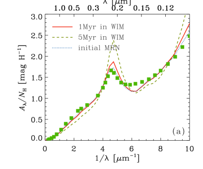
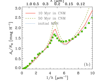
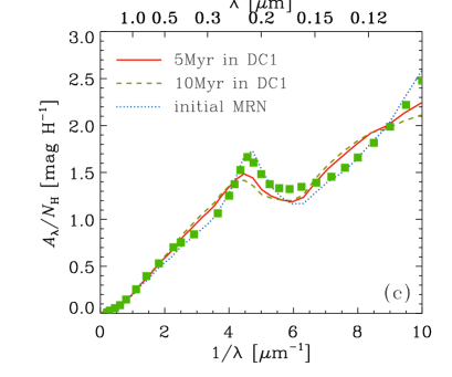
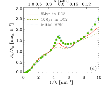
Figure 4: The extinction curves of grains processed in various ISM phases. In each panel, the dotted line represents the initial MRN distribution. (a) $t=1$ Myr and 5 Myr in WIM; (b) $t=10$ Myr and 50 Myr in CNM; (c) $t=5$ Myr and 10 Myr in DC1; and $t=5$ Myr and 10 Myr in DC2 for the solid and dashed lines, respectively. The squares show the data of the observed Milky extinction curve by Pei (1992). In this paper, the extinction is normalized to the hydrogen column density.

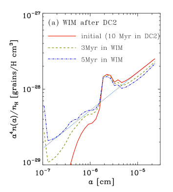
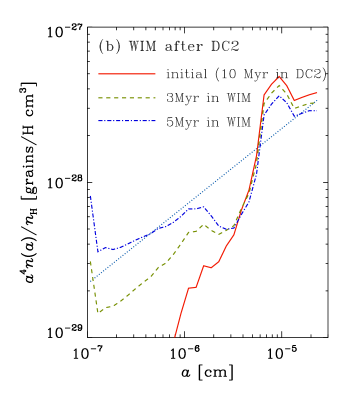
Figure 5: The grain size distributions of (a) silicate and (b) graphite after $t=3$ Myr (dashed line) and $t=5$ Myr (dot-dashed line) in WIM from the initial distribution (solid line), for which the size distribution processed for 10 Myr in DC2 is adopted. The dotted line in each panel shows the MRN distribution.

3.2.1 WIM

The extinction curves of the grains processed in WIM are shown in Fig. 4a. At $t=5$ Myr, the 2175 Å bump is too high and the UV slope is too steep to be consistent with the observed Milky Way extinction curve. Thus, we can conclude that the grains are continuously processed in WIM for no longer than 5 Myr. It is interesting to point out that this timescale is roughly comparable to the recombination timescale of gas with density $\sim 0.1~{}\mathrm{cm}^{-3}$ and temperature $\sim 10^{4}$ K ($\sim 10^{6}$ yr; Spitzer 1978) and to the typical lifetime of massive stars (source of ionizing photons).

3.2.2 CNM

In Fig. 4b, we show the extinction curves in CNM. Because large graphite grains are shattered, the 2175 Å bump becomes high and the UV slope becomes steep. The extinction curves after shattering in CNM do not deviate largely from the observed Milky Way extinction curve within 10 Myr. If grains suffer a longer time of shattering, the extinction curve shows too high a 2175 Å bump and too steep a UV slope to be consistent with the observed extinction curve. However, as noted in Section 3.1, the arguments here are sensitive to the prediction of grain velocities and the assumed value of shattering threshold velocities.

3.2.3 DC

In Figs. 4c and d, we present the extinction curves in DC1 and DC2, respectively. Because the grain size is biased toward large sizes after coagulation, the 2175 Å bump is lower and the UV slope is less steep than the original curve predicted from the MRN size distribution.

The extinction curves in DC2 are more consistent with the observed Milky Way extinction curves than those in DC1 in the following two points. First, the wavelength at the peak of 2175 Å bump changes less in DC2 than in DC1. The observed central wavelengths of 2175 Å bump in various lines of sight in the Milky Way are insensitive to the variation of bump strength (, Cardelli et al.1989). The different behaviours of the 2175 Å bump between DC1 and DC2 come from the “smoothness” of the size distribution around $a\sim\mbox{a few}\times 10^{-6}$ cm: In DC1 the graphite size distribution show a very steep depletion of grains at $a<3\times 10^{-6}$ cm, while in DC2 the depletion of such small grains is not so drastic as in DC1.

Second, the behaviours of $R_{V}$ in terms of the 2175 Å bump and the UV slope are more consistent with the observed Milky Way extinction curves in DC2 than in DC1. The observed Milky Way extinction curves show that a large $R_{V}$ is related to a weak 2175 Å bump and a shallow UV slope (, Cardelli et al.1989). Starting from 3.6 at $t=0$, $R_{V}$ changes to 3.2 ($t=5$ Myr) and 3.1 ($t=10$ Myr) in DC1, while it changes to 4.2 and 4.8 in DC2. Thus, DC1 has a trend opposite to the observed one, while DC2 reproduces a right trend between $R_{V}$, the 2175 Å bump, and the UV slope. Only the grains with $a<4\times 10^{-6}$ cm, whose velocity is below the coagulation threshold velocity, can coagulate in DC1. Since the grain size change in this small size range does not affect the extinction in long wavelengths such as $B$ and $V$ bands, coagulation of larger grains is necessary to change $R_{V}$. This is why $R_{V}$ changes only a little in DC1. In DC2, coagulation to larger grain sizes indeed occurs and $R_{V}$ increases as coagulation proceeds. Considering that there are uncertainties in the threshold velocity for coagulation and in the grain velocities, the success in reproducing qualitatively the trend among $R_{V}$, the 2175 Å bump, and the UV slope in DC2 supports the view that coagulation induced by turbulent motions in dense environments really occurs in the ISM.

4 Discussion

The important features found in the previous section can be summarized as follows.

(i) The largest effect of shattering is seen in WIM, where grains with $a\ga 10^{-6}$ cm are efficiently shattered.

(ii) The largest effect of coagulation is observed in DC around $a\la\mbox{a few}\times 10^{-6}$ cm.

(iii) Grains with $a\ga\mbox{a few}\times 10^{-5}$ cm can be shattered in WNM and graphite grains with $a\ga 10^{-5}$ cm may be quite efficiently destroyed in CNM. These destructions could affect the upper limit of grain size in ISM.

(iv) On the other hand, the lower limit of grain size may be determined by coagulation in DC and MC.

The features (i) and (ii) indicate that once grains are included in WIM or DC, the grain size distribution is significantly modified. It is interesting to note that the shattered grains in (i) and the coagulated grains in (ii) have a similar size. Thus, it is worth investigating if the MRN size distribution can be realized as a balance between (i) and (ii). This point is investigated in Section 4.1.

Regarding the feature (iii), as mentioned in Section 3.2.2, the results in CNM are sensitive to the grain velocities and the shattering thresholds. We leave more careful treatment of shattering in CNM for future work. Shattering in WNM is interesting to investigate, since turbulence in WNM accelerates grains with $a\ga\mbox{a few}\times 10^{-5}$ cm much above the threshold velocity for shattering. This size really matches the upper limit of the grain size distribution (MRN). This point is investigated in Section 4.2.

The issue (iv) has already been investigated and discussed in Section 3.2.3.

4.1 Grain size distributions in diffuse-dense phase exchange

In ISM, mass is exchanged between various phases (McKee & Ostriker, 1977; Ikeuchi, 1988). Thus, it is important to investigate the effects of multi-phase ISM on the evolution of grain size distribution, although the main aim of this paper is to examine the dust processing in individual phases. The largest shattering and coagulation effects are seen in WIM and DC, respectively, and we here examine the dust processing in both WIM and DC to address a possible importance of multi-phase ISM in determining the grain size distribution. For DC, we adopt DC2 because of the success in explaining the trend of $R_{V}$ in terms of the UV slope and the 2175 Å bump (Section 3.2.3).

We start from the size distribution of grains processed in DC2 for 10 Myr. Then, we apply the condition of WIM. In Fig. 5, we show the results at $t=3~{}\mathrm{Myr}$ and 5 Myr in WIM. Around 5 Myr, the number of small grains is recovered to the level of the MRN distribution. In other words, if grains pass their lifetimes in WIM more than in DC, the grains are shattered too much to be consistent with the MRN distribution. This implies a short lifetime of WIM. Combining this short lifetimes of WIM with a theoretically implied timescale for the phase exchange ($\mbox{a few}\times 10^{7}$–$10^{8}$ yr; Section 2.5), we obtain a picture that a large fraction of warm medium is in a neutral form and a certain small fraction is ionized. It is interesting to point out that such a short timescale is consistent with the recombination timescale as mentioned in Section 3.2.1.

The corresponding extinction curves are shown in Fig. 6. The Milky Way extinction curve is indeed recovered by the phase exchange. This demonstrates that it is really possible to reproduce the Milky Way extinction curve by considering dust grains processed in multiphase medium.

The above phase exchange model is too simple, and the realistic ISM has more continuous density distribution and more complicated structure of turbulence (Wada & Norman, 2001). Such complexity should tend to eliminate the specific features such as accumulation of grains around $a\sim\mbox{a few}\times 10^{-6}$ cm in DC and selective grain destruction at $a\sim 10^{-6}$ cm in WIM. Thus, we expect that the grain size distribution becomes smoother in realistic ISM than we calculate in this paper.

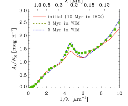
Figure 6: The extinction curves calculated for the size distributions in Fig. 5. The solid line represents the initial size distribution (10 Myr in DC2), and the dashed and dot-dashed lines show the extinction curves at $t=3$ Myr and 5 Myr in WIM, respectively.

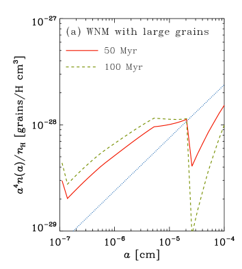
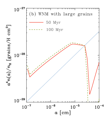
Figure 7: The grain size distributions of (a) silicate and (b) graphite after $t=50$ Myr (solid line) and $t=100$ Myr (dashed line) in WIM for the MRN size distribution extending up to $a=10^{-4}$ cm as the initial condition (dotted line).

4.2 Upper and lower limits of grain size

According to MRN, the upper grain radius is $\sim 0.25~{}\mu$m (see also Kim et al. 1994). Coagulation has negligible influence on grains larger than $a\sim 0.2~{}\mu$m both for silicate and for graphite because they generally obtain larger velocity than the coagulation thresholds. Thus, if there is no grain with $a\ga 0.2~{}\mu$m initially, it is not possible to make such large grains by coagulation in ISM.

Even if grains larger than $a\sim 0.2~{}\mu$m form by condensation in stellar ejecta, shattering could destroy such large grains. Nozawa et al. (2003) show that silicon grains with $a>0.2~{}\mu$m form in Type II supernovae. In the outflows from evolved late-type stars, the grain radius is expected to become of order $\sim 0.1~{}\mu$m (Gail & Sedlmayr, 1999), and grains with $a\ga 0.2~{}\mu$m may have a chance to form. It is interesting to note that grains with $a\ga 0.2$–0.3 $\mu$m are accelerated above the shattering threshold in WNM. Thus, shattering in WNM may play a central role in determining the upper limit of the grain size in ISM.

In order to examine whether or not shattering in WNM really plays a role in determining the upper limit of the grain size, we perform a test by adopting an initial grain size distribution extending up to $a=1~{}\mu$m with the total mass of grains conserved. Then the evolution of the grain size distribution is calculated by applying the conditions in WNM. Fig. 7 shows the results. We observe that the grains with $a\ga 0.2$–0.3 $\mu$m are significantly shattered in 50 Myr. Thus, shattering in WNM is a strong candidate for the determining mechanism of the upper limit of grain size.

In Fig. 8, we show the corresponding extinction curves. The initial extinction curve is significantly lower than the observed one because large grains tend to have low mass absorption coefficients. However, after 50 Myr, the level of the extinction is already consistent with the Milky Way curve. This means that shattering of large grains in WNM is efficient enough to reproduce the upper grain size consistent with the observed Milky Way extinction curve.

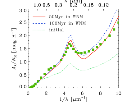
Figure 8: The extinction curves calculated for the size distributions in Fig. 7. The dotted line represents the initial extinction curve (MRN size distribution extending up to $a=10^{-4}$ cm). The solid and dashed lines show the extinction curves of grains at $t=50$ Myr and $t=100$ Myr in WNM, respectively.

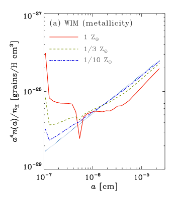
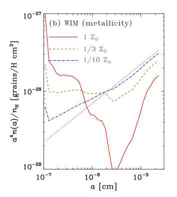
Figure 9: The grain size distributions of (a) silicate and (b) graphite at $t=10$ Myr in WIM. The solid, dashed, dot-dashed lines show $Z=1$, 1/3 and 1/10 $\mathrm{Z}_{\odot}$, respectively. The dust abundance (vertical axis) of the dashed and dot-dashed lines are multiplied by 3 and 10, respectively, to offset the low dust abundances.

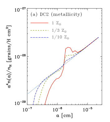
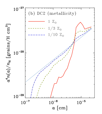
Figure 10: Same as Fig. 9 but in DC2.

4.3 In the context of galaxy evolution

The efficiencies of shattering and coagulation are affected by the grain abundance. This indicates that metal-poor galaxies, which are generally poor in dust content (Issa et al., 1990), have different grain size distributions. Here we examine the metallicity dependence of shattering and coagulation. We assume that the dust-to-gas ratio is proportional to the metallicity $Z$; that is, we adopt ${\cal R}=4.0\times 10^{-3}Z/\mathrm{Z}_{\odot}$ and $3.4\times 10^{-3}Z/\mathrm{Z}_{\odot}$ for silicate and graphite, respectively, in equation (25). In other words, the dust density in the ISM is proportional to the metallicity, and we expect that the effects of shattering and coagulation become weak as the metallicity decreases. The turbulence model and the grain velocities are not changed, which means that we implicitly assume that the parameters listed in Table 1 are fixed.

We test WIM and DC, where shattering and coagulation, respectively, are the most efficient among the various phases. In Fig. 9, we show the grain size distributions in WIM at $t=10$ Myr. We apply a longer timescale than adopted in the other part of this paper to enhance the effect of shattering. We observe that the shattering effect is significantly reduced at $1/10~{}\mathrm{Z}_{\odot}$. The same is true for coagulation in DC as shown in Fig. 10, where we adopt DC2 because of the success in reproducing the trend of $R_{V}$ in terms of the UV slope and the 2175 Å bump (Section 3.2.3). Thus, as the metallicity decreases, the relative importance of processing by interstellar turbulence becomes minor in determining the grain size distribution. This indicates that the initial grain size distribution at the grain formation in stellar ejecta is relatively preserved in metal-poor galaxies (typically $Z<1/10~{}\mathrm{Z}_{\odot}$), although we should keep in mind that there are other processes, such as interstellar shocks by supernovae, which could modify the grain size distribution in any metallicity.

4.4 Toward the grain evolution in protoplanetary discs

The condition of turbulence in the circumstellar discs is still unclear. Let us consider protoplanetary discs. According to Nomura & Nakagawa (2006), turbulence is very weak ($\delta V\sim 0.01\mbox{--}0.1c_{\mathrm{s}}$, where $c_{\mathrm{s}}$ is the sound speed). The acceleration by turbulence will be marginal in this case, and grain motions are more likely to be Brownian. As a result coagulation is at least as efficient as in DC. As shown in Figs. 2 and 3, small grains with $a\la 10^{-6}$ cm are strongly depleted in DC because of coagulation. Thus, we can justify that the grain size distribution in protoplanetary discs is biased to radii $\ga 10^{-6}$ cm. Moreover, because grain velocities are expected to be lower than the coagulation threshold even at $a>10^{-6}$ cm, grains grow further.

As shown by Sano et al. (2000), the grain size in protoplanetary discs is important in determining the unstable regions for magnetorotational instability, which induces MHD turbulence (Balbus & Hawley, 1998). Consequently the grain size distribution is further affected by the presence/absence of the turbulent motion determined by the instability/stability condition. The coupling between turbulence and grain size is interesting to investigate as a future work.

5 Summary

We have investigated the effects of shattering and coagulation on the dust size distribution in turbulent ISM, adopting the typical velocities of dust grains as a function of grain size from YLD04. By using a scheme of grain shattering and coagulation which we have developed in this paper based on JTH96 and Chokshi et al. (1993), we have calculated the evolution of grain size distribution in turbulent ISM. Since large grains tend to have large velocities because of decoupling from small-scale turbulent motions, large grains tend to be shattered. On the other hand, because of small surface-to-volume ratio, large grains require more time to be destroyed.

Large shattering effects are indeed seen in WIM for grains with $a\ga\mbox{a few}\times 10^{-6}$ cm. In the supernova shocks, such small grains are decelerated quickly by gas drag and larger grains tend to be shattered more efficiently (JTH96). Graphite grains are predicted to be shattered also in CNM, but the result in CNM is sensitive to the threshold velocity for shattering. Coagulation significantly modifies the grain size distribution in DC. In fact, the correlation among $R_{V}$, the carbon bump, and the UV slope in the observed Milky Way extinction curves is qualitatively reproduced by the coagulation in DC. We have also shown that the upper limit of the grain size in ISM can be determined by the shattering in WNM.

If a large fraction of ISM experiences either WIM or DC, the grain size distribution in ISM may be determined by a balance between shattering in WIM and coagulation in DC. Considering that the effects of shattering and coagulation become small in metal-poor environments, the regulation mechanism of grain size distribution is quantitatively different between metal-poor and metal-rich environments.

References

- Arons & Max (1975) Arons, J., & Max, C. E. 1975, ApJ, 196, L77
- Balbus & Hawley (1998) Balbus, S. A., & Hawley, J. F. 1998, Rev. Mod. Phys., 70, 1
- Beresnyak & Lazarian (2008) Beresnyak, A., & Lazarian, A. 2008, ApJ, 682, 1070
- Bianchi & Schneider (2007) Bianchi, S., & Schneider, R. 2007, MNRAS, 378, 973
- Blitz & Shu (1980) Blitz, L, & Shu, F. H. 1980, ApJ, 238, 148
- Blum (2000) Blum, J. 2000, Space Sci. Rev., 92. 265
- Bohlin, Savage, & Drake (1978) Bohlin, R. C., Savage, B. D., & Drake, J. F. 1978, ApJ, 224, 291
- Bohren & Huffman (1983) Bohren, C. F., & Huffman, D. R. 1983, Absorption and Scattering of Light by Small Particles, Wiley, New York
- Borkowski & Dwek (1995) Borkowski, K. J., & Dwek, E. 1995, ApJ, 454, 254
- (10) Cardelli, J. A., Clayton, G. C., & Mathis, J. S. 1989, ApJ, 345, 245
- Chandran (2005) Chandran, B. 2005, Phys. Rev. Lett., 95, 265004
- Cho & Lazarian (2002) Cho, J., & Lazarian, A. 2002, Phys. Rev. Lett., 88, 245001
- Cho & Lazarian (2003) Cho, J., & Lazarian, A. 2003, MNRAS, 345, 325
- Chokshi et al. (1993) Chokshi, A., Tielens, A. G. G. M., & Hollenbach, D. 1993, ApJ, 407, 806
- Dominik, Gail, & Sedlmayr (1989) Dominik, C., Gail, H.-P., & Sedlmayr, E. 1989, A&A, 223, 227
- Dominik & Tielens (1997) Dominik, C., & Tielens, A. G. G. M. 1997, ApJ, 480, 647
- Draine (1985) Draine, B. T. 1985, in Black D. C., Matthews M. S., eds, Protostars and Planets II, Univ. Arizona Press, Tucson, p. 621
- Draine & Lee (1984) Draine, B. T., & Lee, H. M. 1984, ApJ, 285, 89
- Dwek & Scalo (1980) Dwek, E., & Scalo, J. M. 1980, ApJ, 239, 193
- Elmegreen (2000) Elmegreen, B. G. 2000, ApJ, 530, 277
- Fitzpatrick & Massa (2007) Fitzpatrick, E. L., & Massa, D. 2007, ApJ, 663, 320
- Gail & Sedlmayr (1999) Gail, H.-P., & Sedlmayr, E. 1999, A&A, 347, 594
- Gehrz (1989) Gehrz, R. D. 1989, in Allamandola L. J., Tielens A. G. G. M., eds, Proc. IAU Symp. 135, Interstellar Dust. Kluwer, Dordrecht, p. 445
- Goldreich & Sridhar (1995) Goldreich, P., Sridhar, S. 1995, ApJ, 438, 763
- Hartmann (2003) Hartmann, L. 2003, ApJ, 585, 398
- Hellyer (1970) Hellyer, B. 1970, MNRAS, 148, 383
- Hirashita & Ferrara (2002) Hirashita, H., & Ferrara, A. 2002, MNRAS, 337, 921
- Hirashita & Kamaya (2001) Hirashita, H., & Kamaya, H. 2001, AJ, 120, 728
- Ikeuchi (1988) Ikeuchi, S. 1988, Fundam. Cosmic Phys., 12, 255
- Issa et al. (1990) Issa, M. R., MacLaren, I., & Wolfendale, A. W. 1990, A&A, 236, 237
- Jones, Tielens, & Hollenbach (1996) Jones, A. P., Tielens, A. G. G. M., & Hollenbach, D. J. 1996, ApJ, 469, 740 (JTH96)
- Jones et al. (1994) Jones, A. P., Tielens, A. G. G. M., Hollenbach, D. J., & McKee, C. F. 1994, ApJ, 433, 797
- Kawamura et al. (2007) Kawamura, A., Minamidani, T., Mizuno, Y., Onishi, T., Mizuno, N., Mizuno, A., & Fukui, Y. 2007, in Elmegreen B., Palous J. eds, Proc. IAU Symp. 237, Triggered Star Formation in a Turbulent ISM, Cambridge University Press, Cambridge p. 101
- Kim et al. (1994) Kim, S.-H., Martin, P. G., & Hendry, P. D. 1994, ApJ, 422, 164
- Kusaka et al. (1970) Kusaka, T., Nakano, T., & Hayashi, C. 1970, Prog. Theor. Phys., 44, 1580
- Lazarian & Vishniac (1999) Lazarian, A., & Vishniac, E. 1999, ApJ, 517, 700
- Lazarian & Yan (2002) Lazarian, A., & Yan, H. 2002, ApJ, 566, L105
- Li & Draine (2001) Li, A., & Draine, B. T. 2001, ApJ, 554, 778
- Mathis et al. (1977) Mathis, J. S., Rumpl, W., & Nordsieck, K. H. 1977, ApJ, 217, 425 (MRN)
- Maiolino et al. (2004) Maiolino, R., Schneider, R., Oliva, E., Bianchi, S., Ferrara, A. Mannucci, F., Pedani, M., & Roca Sogorb, M. 2004, Nature, 431, 533
- McKee et al. (1987) McKee, C. F., Hollenbach, D. J., Seab, C. G., & Tielens, A. G. G. M. 1987, ApJ, 318, 674
- McKee & Ostriker (2007) McKee, C. F., & Ostriker, E. C. 2007, ARA&A, 45, 565
- McKee & Ostriker (1977) McKee, C. F., & Ostriker, J. P. 1977, ApJ, 218, 148
- Myers & Goodman (1988) Myers, P. C., & Goodman, A. A. 1988, ApJ, 326, L27
- Noll & Pierini (2005) Noll, S., & Pierini, D. 2005, A&A, 444, 137
- Nomura & Nakagawa (2006) Nomura, H., & Nakagawa, Y. 2006, ApJ, 640, 1099
- Nozawa et al. (2003) Nozawa, T., Kozasa, T., Umeda, H., Maeda, K., & Nomoto, K. 2003, ApJ, 598, 785
- Nozawa et al. (2007) Nozawa, T., Kozasa, T., Habe, A., Dwek, E., Umeda, H., Tominaga, N., Maeda, K., & Nomoto, K. 2007, ApJ, 666, 955
- O’Donnell & Mathis (1997) O’Donnell, J. E., & Mathis, J. S. 1997, ApJ, 479, 806
- Ossenkopf (1993) Ossenkopf, V. 1993, A&A, 280, 617
- Palla & Stahler (2002) Palla, F., & Stahler, S. W. 2002, ApJ, 581, 1194
- Pei (1992) Pei, Y. C., 1992, ApJ, 395, 130
- Sano et al. (2000) Sano, T., Miyama, S. M., Umebayashi, T., & Nakano, T. 2000, ApJ, 543, 486
- Spangler & Minton (1996) Spangler, S. R., & Minton, A. H. 1996, ApJ. 458, 194
- Spitzer (1978) Spitzer, L., Jr 1978, Physical Processes in the Interstellar Medium, New York, Wiley
- Suzuki, Lazarian & Beresnyak (2007) Suzuki, T. K., Lazarian, A., Beresnyak, A. 2007, ApJ, 662, 1033
- (57) Takagi, T., Vansevičius, V., & Arimoto, N. 2003, PASJ, 55, 385
- Takeuchi et al. (2005) Takeuchi, T. T., Ishii, T. T., Nozawa, T., Kozasa, T., & Hirashita, H. 2005, MNRAS, 362, 592
- Tielens et al. (1994) Tielens, A. G. G. M., McKee, C. F., Seab, C. G., & Hollenbach, D. J. 1994, ApJ, 431, 321
- Todini & Ferrara (2001) Todini, P., & Ferrara, A. 2001, MNRAS, 325, 726
- Völk et al. (1980) Völk, H. J., Jones, F. C., Morfill, G. E., & Röser, S. 1980, A&A, 85, 316
- Wada & Norman (2001) Wada, K., & Norman, C. A. 2001, ApJ, 547, 172
- Weingartner & Draine (2001) Weingartner, J. C., & Draine, B. T. 2001, ApJ, 548, 296
- Yan & Lazarian (2003) Yan, H., & Lazarian, A. 2003, ApJ, 592, L33
- Yan et al. (2004) Yan, H., Lazarian, A., & Draine, B. T. 2004, ApJ, 616, 895 (YLD04)