Resonant flavor conversion of supernova neutrinos and neutrino parameters

Abstract

The unknown neutrino parameters may leave detectable signatures in the supernova (SN) neutrino flux. However, even the contribution from the MSW flavor transition alone could cause ambiguity in the interpretation to the neutrino signals because of the uncertain local density profile of the SN matter and the model-dependent SN neutrino spectral parameters. A specific parametrization to the unknown local density profile is proposed in this work, and the contribution from the standard MSW effect is investigated through a multi-detector analysis of the SN neutrinos. In establishing the model-independent scheme, results based on the existing spectral models are included. The limitation of the analysis is also discussed.

I Introduction

As a distinctive type of the neutrino source, the core-collapse supernova (SN) provides a rich physical content that is lacking in the terrestrial environment. With its unique production and detection processes, the neutrino burst from a SN has long been considered as one of the promising tools for probing the unknown neutrino intrinsic parameters dighe:00 ; ref2 ; ref3 ; ref4 ; ref5 ; ref6 ; ref7 , in particular, the neutrino mass hierarchy and the tiny mixing angle $\theta_{13}$. However, difficulties also arise from the complexity caused by the unavoidable astrophysical uncertainties, which could lead to ambiguous interpretations of the observed events.

The existing paradigm for the neutrino MSW flavor conversion in a SN has been established with the assumption of small neutrino self interaction. However, a possible new paradigm has been shaped in recent years. The argument is that, in addition to the standard MSW effect, the neutrinos may encounter certain non-MSW effects in the SN environment when the neutrino number density is extremely high. These not so well-known effects may be independent of the MSW effect and may introduce additional factors that alter the efficiency of the neutrino flavor transition. The current consensus is that both types of effects could contribute to the flavor transition and should all be included in the more complete analysis of the SN neutrino signals.

Even the standard treatment of the MSW flavor conversion alone is not immune from ambiguity. The uncertain local density profile of the SN matter and the undetermined neutrino spectral parameters, such as the average energy and the luminosity of each neutrino flavor, are the crucial factors involved in the MSW effect of the SN neutrinos. However, an analysis based on the simple global density model: $\rho\sim r^{-3}$, which is widely adopted in the literature, could lose the generality if the variation of the local density shape near the resonance is not taken into account. With these uncertain factors, it is worth while to investigate how the contribution from the standard MSW effect should be modified in analyzing the SN neutrino signals, unless the overall contribution from the non-MSW effects is much greater than that from the MSW effect.

The resonant neutrino flavor transition in a SN and in Earth would in principle give rise to observable signatures that reflect the properties of neutrino parameters. The unknown local density profile of SN matter near the resonance takes part in the adiabaticity parameter of the level crossing, and plays a role in the determination of transition probabilities. In fact, the adiabaticity of the level crossing could vary abruptly with the local density profile in certain neutrino parameter space. In addition, the knowledge to the primary spectrum for each neutrino flavor is essential in assessing the efficiency of neutrino flavor conversion. Various mixing scenarios, which arise from the uncertain SN physics, the possible neutrino mass hierarchies, and the uncertain magnitude of $\theta_{13}$ lead to distinct neutrino survival probabilities. An analysis of the observed neutrino signals should, in principle, be able to single out the working scenario.

The promising features of the multi-detector experiments have been well recognized ls:01 ; mirizzi ; dighe:03 ; minakata:08 ; sf:08 . With the uncertain local density profile and the spectral parameters, this work investigates the potential signatures that may be related to the contribution from the MSW effect in a multi-detector analysis of the SN neutrinos. As suggested by the previous work chiu06 ; chiu07 , the consequences due to the uncertain local density profile near the resonance can be accounted for by the adoption of independent and variable power-law density functions $\rho(r)=c_{k}r^{n_{k}}$. However, the calculations in Ref. 13 and 14 are performed under the assumption of nearly constant $c_{k}$, which is similar to that adopted in the usual analysis based on $\rho(r)=cr^{-3}$. In the present work, the key improvement in dealing with the variable density profile is the establishment of variable $c_{k}$, which reproduces reasonable densities that agree with the numerical simulations at a wide range of the radial location. With the more general parametrization of the density function, this work is further devoted to analyzing the expected neutrino events at two water Cherenkov detectors. Focus is aimed at the modified contribution from the MSW effect. Certain physical observables derived from the expected event rates at the two detectors are proposed as the discriminators of various transition scenarios for the MSW resonance. In searching for the model-independent properties of the observables, three existing SN neutrino spectral models proposed by the Garching group Ga ; Gb and the Lawrence Livermore groupLL are adopted in the calculation.

II Uncertain density profile of SN matter

There is no definite way of modeling the practically unknown local variation of density profile. Considering the narrow thickness of the resonant layer, as compared to that of the whole scope of the SN matter distribution, the density profile with a form of variable power-law in each resonant layer would be a reasonable simplification that accounts for the possible dynamical consequences. The essence of this approximation is that the power characterizing the density profile in each resonant layer is allowed to vary independently: $\rho(r)\sim c_{l}r^{n_{l}}$ for the lower resonance layer, and $\rho(r)\sim c_{h}r^{n_{h}}$ for the higher resonance layer, where the factor $c_{k}$ denotes the magnitude of the profile $r^{n_{k}}$, with $k=l$ or $h$.

In this present work, the density profile in the resonance layer is parameterized as

$$\rho(r)=[\frac{c}{R_{0}^{3}}][\frac{r}{R_{0}}]^{n_{k}},$$ (1)

where $c$ is a mass scale, and $R_{0}$ is a distance scale, which is conveniently taken as the solar radius, $R_{0}\simeq 6.96\times 10^{10}$ cm. With the variable $n_{k}$, an important criterion for a reliable parametrization of the density profile is that the predicted density at a specific radial location agrees with that given by the numerical simulation, at least in order of magnitude. This suggests that in Eq.(1) the variation of $n_{k}$ is accompanied by the variation of $c$ at a different location. One may thus write the density profile in a more convenient form as

$$\rho(r)=[\frac{c_{0}}{R_{0}^{3}}][\frac{c}{c_{0}}][\frac{r}{R_{0}}]^{n_{k}},$$ (2)

where $c_{0}$ is a constant mass scale, and $c_{0}/R_{0}^{3}$ is a reference density scale. In the typical model with a fixed power, $\rho(r)=cr^{-3}$, the magnitude of $c$ varies weaklykuo88 : $10^{31}g<c<15\times 10^{31}g$ in the density range $10^{-5}g/cm^{3}<\rho<10^{12}g/cm^{3}$. For variable $n_{k}$ near a given location, however, the mass scale $c$ may vary by several orders of magnitude so as to reproduce reasonable density at this specific radial location. Note that with this variable parametrization of the density profile, the choice of $c_{0}$ does not alter the results since the variation of the mass scale is represented by $c$. In this present analysis we shall adopt the value $c_{0}=7.0\times 10^{31}g$, which is simply the mean value of $c$ in the typical density model. The variables $c$ and $r$ may be rewritten as $c/c_{0}=X$ and $r/R_{0}=Z$, respectively, and the density profile becomes

$$\rho(r)=[\frac{c_{0}}{R_{0}^{3}}]XZ^{n_{k}}.$$ (3)

By fitting the predicted densities with the numerical resultswoosley-1 ; woosley-2 ; sato:03 at different radial locations, this parametrization leads to an approximate relation that regulates the variation of $c$, $r$, and $n_{k}$:

$$X\sim\frac{1}{2}Z^{-(n_{k}+3)}.$$ (4)

As summarized in the following, the variation of $n_{k}$ can lead to non-trivial effects on the crossing probabilities at the resonance. One may first write the electron number density $N_{e}(r)$ for a typical core collapse SN as

$$N_{e}(r)=\rho(r)[Y_{e}/m_{n}],$$ (5)

where the electron number per baryon $Y_{e}=1/2$ is adopted, and $m_{n}$ is the baryon mass. The adiabaticity parameter for the resonant transition, defined askuo89

$$\gamma_{k}\equiv\frac{\delta m^{2}_{ij}\sin^{2}2\theta_{ij}}{2E\cos 2\theta_{ij}|\frac{1}{N_{e}}\frac{dN_{e}}{dr}|_{0}},$$ (6)

becomes

$$\gamma_{k}=\frac{1}{2|n_{k}|}[\frac{\delta m^{2}_{ij}}{E}][\frac{\sin^{2}2\theta_{ij}}{\cos 2\theta_{ij}}][(\delta m^{2}_{ij}/E)\frac{\cos 2\theta_{ij}}{\sqrt{2}G_{F}(\frac{Y_{e}}{m_{n}})(\frac{c_{0}}{R_{0}^{3}})}]^{\frac{1}{n_{k}}}R_{0}Z_{0}^{(1+\frac{3}{n_{k}})},$$ (7)

where $\delta m^{2}_{ij}\equiv m^{2}_{i}-m^{2}_{j}$, $\theta_{ij}$ is the mixing angle between the eigenstates $\nu_{i}$ and $\nu_{j}$, $G_{F}$ is the Fermi constant, $E$ is the neutrino energy, and $Z_{0}=r_{0}/R_{0}$ indicates the location of resonance. Note that $|(1/N_{e})(dN_{e}/dr)|_{0}$ is evaluated at the resonance, where

$$(N_{e})_{0}=\frac{\delta m^{2}_{ij}\cos 2\theta_{ij}}{2\sqrt{2}G_{F}E}.$$ (8)

The adiabaticity parameter $\gamma_{k}$ appears in the level crossing probability $P_{k}$ (with $k=l$ or $h$) as:

$$P_{k}=\frac{\exp[-\frac{\pi}{2}\gamma_{k}F_{k}]-\exp[-\frac{\pi}{2}\gamma_{k}\frac{F_{k}}{\sin^{2}\theta_{ij}}]}{1-\exp[-\frac{\pi}{2}\gamma_{k}\frac{F_{k}}{\sin^{2}\theta_{ij}}]},$$ (9)

where $F_{k}$ is the correction factor to a non-linear profile. The origin of Eq. (9) and the correction function $F_{k}$ can be found in, $e.g.$, Ref. 22. We shall adopt $\delta m^{2}_{21}=7.0\times 10^{-5}$ eV², $|\delta m^{2}_{13}|=3.0\times 10^{-3}$ eV², and $\sin^{2}2\theta_{12}=0.81$ in the calculation. With a given radial location for the resonance, it can be verified that the adiabaticity parameter $\gamma_{k}$, and thus the neutrino survival probability, vary weakly with the energy $E$, as compared to the influences from the variations of $n_{k}$ and $\theta_{13}$. This result suggests that one may simply adopt the average neutrino energies, $e.g.$, $E_{\nu_{e}}=12$ MeV and $E_{\bar{\nu}_{e}}=15$ MeV, in the following calculation for the neutrino transition probability in SN. The energy dependence would only appear in calculating the Earth effect.

III Survival probabilities and scenarios for neutrino parameters

When the neutrinos arrive at Earth, the survival probabilities for $\nu_{e}$ and $\bar{\nu}_{e}$ are given respectively by

$$P_{nor}=U_{e1}^{2}P_{l}P_{h}+U_{e2}^{2}(1-P_{l})P_{h}+U_{e3}^{2}(1-P_{h}),$$ (10)

$$\bar{P}_{nor}=U_{e1}^{2}(1-\bar{P}_{l})+U_{e2}^{2}\bar{P}_{l},$$ (11)

for the normal hierarchy, and

$$P_{inv}=U_{e2}^{2}(1-P_{l})+U_{e1}^{2}P_{l},$$ (12)

$$\bar{P}_{inv}=U_{e2}^{2}\bar{P}_{l}\bar{P}_{h}+U_{e1}^{2}(1-\bar{P}_{l})\bar{P}_{h}+U_{e3}^{2}(1-\bar{P}_{h}),$$ (13)

for the inverted hierarchy, where $P_{h}(\bar{P}_{h})$ and $P_{l}(\bar{P}_{l})$ represent the higher and the lower level crossing probabilities for $\nu_{e}(\bar{\nu}_{e})$, respectively, and $U_{ei}$ is the element of the mixing matrix.

Figure 1: The rapid variation of $P_{h}$ as functions of $\sin^{2}2\theta_{13}$ for $n_{h}=-8$ and $n_{h}=-2$.

In calculating the above level crossing probabilities, it should be emphasized that both the higher and the lower level crossings occur in the $\nu$ sector for the normal hierarchy, while the higher crossing occurs in the $\bar{\nu}$ sector and the lower crossing occurs in the $\nu$ sector if the mass hierarchy is inverted. One thus needs to calculate $P_{h}$ and $P_{l}$ in Eq.(10) for the normal hierarchy, and $\bar{P}_{h}$ in Eq. (13) and $P_{l}$ in Eq.(12) for the inverted hierarchy at the individual resonance. Note that since the antineutrinos do not encounter the resonance at the location where the neutrinos cross the lower resonance, the crossing probability $\bar{P}_{l}$ for both hierarchies in Eq.(11) and Eq.(13) is vanishing: $\bar{P}_{l}=0$. In addition, it can be verified that the adiabaticity parameter $\gamma_{l}$ at the lower resonance is very large, $\gamma_{l}>10^{2}$. This suggests that the lower resonance is adiabatic for both the mass hierarchies: $\gamma_{l}\gg 1$, which leads to $P_{l}\sim 0$.

On the other hand, to show that the variation of $n_{h}$ and $\theta_{13}$ leads to non-trivial structures of $P_{h}$ in the $n_{h}-\theta_{13}$ parameter space, we first estimate the typical density near the location of the higher resonance. Using Eqs.(5) and (8), the density at resonance is given by

$$\rho_{res}=\frac{\delta m_{31}^{2}\cos 2\theta_{13}}{[2\sqrt{2}G_{F}E][Y_{e}/m_{n}]},$$ (14)

which leads to $\rho_{res}\simeq 3\times 10^{3}g/cm^{3}$ with small $\theta_{13}$. This density corresponds to an approximate location of resonance $r_{0}/R_{0}=Z_{0}\sim 0.03$ according to the numerical results woosley-1 ; woosley-2 ; sato:03 . It follows from Eqs.(7) and (9) that the crossing probability $P_{h}$ is in general non-adiabatic ($P_{h}\sim 1$) for $\sin^{2}2\theta_{13}<10^{-5}$. This leads to $P_{nor}=P_{inv}=|U_{e2}|^{2}\sim 0.3$, as can be checked using Eqs. (10) and (12). In addition, it can be verified that $P_{inv}$ remains constant through out the parameter space with $P_{inv}\sim 0.3$. However, the probability $P_{nor}$ varies with both $n_{h}$ and $\theta_{13}$ near $\sin^{2}2\theta_{13}\sim 10^{-5}-10^{-4}$ since $P_{h}$ drops rapidly from $P_{h}\sim 1$ (non-adiabatic) to $P_{h}\sim 0$ (adiabatic) within a narrow region of the parameter space. It follows that $P_{nor}$ drops from $P_{nor}\sim 0.3$ to $P_{nor}=|U_{e3}|^{2}\ll 1$. This property distinguishes $P_{nor}$ from $P_{inv}$. As an illustration, we show $P_{h}$ as a function of $\sin^{2}2\theta_{13}$ for $n_{h}=-2$ and $n_{h}=-8$ in Fig. 1.

Table 1: The survival probabilities for $\nu_{e}$ and $\bar{\nu}_{e}$, the possible neutrino mass hierarchy, and the function $g(n_{h},\theta_{13})$ as predicted by the specific scenarios. The uncertainty in the power of the local density profile can alter the predicted bound of $\theta_{13}$ through the function $g(n_{h},\theta_{13})$.

		$P$		$\bar{P}$		mass hierarchy		$g(n_{h},\theta_{13})$
$(a)$		$|U_{e3}|^{2}=\sin^{2}\theta_{13}$		$|U_{e1}|^{2}\simeq\cos^{2}\theta_{12}$		normal		$>1$
$(b)$		$|U_{e2}|^{2}\simeq\sin^{2}\theta_{12}$		$|U_{e3}|^{2}=\sin^{2}\theta_{13}$		inverted		$>1$
$(c)$		$|U_{e2}|^{2}\simeq\sin^{2}\theta_{12}$		$|U_{e1}|^{2}\simeq\cos^{2}\theta_{12}$		both		$<1$

It is then reasonable to represent the narrow borderline between the adiabatic crossing ($P_{h}\sim 0$) and the non-adiabatic crossing ($P_{h}\sim 1$) by the condition $P_{h}=1/2$, which implies (with small $\theta_{13}$)

$$\exp[-\frac{\pi}{2}\gamma_{h}F_{h}]\sim\frac{1}{2}.$$ (15)

Equations (7) and (15) lead to $\frac{\pi}{2\ln 2}\gamma_{h}\equiv g(n_{h},\theta_{13})\sim 1$, with

$$g(n_{h},\theta_{13}) = \frac{\pi}{4(\ln 2)}\frac{1}{|n_{h}|}[\frac{|\delta m^{2}_{31}|}{E}][\frac{\sin^{2}2\theta_{13}}{\cos 2\theta_{13}}]$$ (16)

$$\times[(|\delta m^{2}_{31}|/E)\frac{\cos 2\theta_{13}}{\sqrt{2}G_{F}(\frac{Y_{e}}{m_{n}})(\frac{c_{0}}{R_{0}^{3}})}]^{\frac{1}{n_{h}}}R_{0}Z_{0}^{(1+\frac{3}{n_{h}})},$$

where $Z_{0}=0.03$, $R_{0}=6.96\times 10^{10}$ cm, and $F_{h}\sim 1$ (for small $\theta_{13}$). Thus, how the uncertainty in $n_{h}$ alters the predicted bound for $\theta_{13}$ is regulated by the function $g(n_{h},\theta_{13})$, and depends on whether the parameters $n_{h}$ and $\theta_{13}$ result in $g(n_{h},\theta_{13})<1$ or $g(n_{h},\theta_{13})>1$. The similar properties for $\bar{P}_{nor}$ and $\bar{P}_{inv}$ also can be derived from Eqs. (7), (9), (11), and (13). As a brief summary, one notes that with the formulation and the chosen input parameters, (i) $P_{l}=0$, and $\bar{P}_{l}=0$, and (ii) $P_{h}=\bar{P}_{h}=1$ if $g(n_{h},\theta_{13})<1$, while $P_{h}=\bar{P}_{h}=0$ if $g(n_{h},\theta_{13})>1$.

Figure 2: The adiabaticity parameters is modified for a finite resonance layer, within which the density and the mass scale $c$ are both variable. The contours for $g(n_{h},\theta_{13})\equiv\frac{\pi}{2\ln 2}\gamma_{h}=1$ are shown in the $n_{h}-\theta_{13}$ space with $Z=Z_{0}$, $Z=Z_{0}(1+10\%)$, and $Z=Z_{0}(1-10\%)$, where $Z_{0}=0.03$. Note that since the estimated deviation ($<2.7\%$) is barely observable in the parameter space, an exaggerated uncertainty of $10\%$ is shown here for the purpose of illustration and comparison. We may conclude that this small deviation does not alter the general picture of the analysis.

In terms of the survival probabilities $P$ and $\bar{P}$ for $\nu_{e}$ and $\bar{\nu}_{e}$, respectively, the uncertain local density profile, the possible mass hierarchies, and the undetermined mixing angle $\theta_{13}$ together lead to three possible combinations of ($P$,$\bar{P}$), as indicated by $(a)$, $(b)$, and $(c)$ in Table 1. In general, separating the scenarios is unlikely if $\sin^{2}2\theta_{13}<10^{-5}$ since $P_{nor}$ and $P_{inv}$, as well as $\bar{P}_{nor}$ and $\bar{P}_{inv}$, cannot be distinguished. In addition, there is a non-trivial dependence of $P$ and $\bar{P}$ on both $n_{h}$ and $\theta_{13}$ near $\sin^{2}2\theta_{13}\sim 10^{-4}$. This implies that establishing a better lower bound for $\theta_{13}$ relies on whether the uncertainty of $n_{h}$ in this region of parameter space can be reduced. Based on Table 1, we discuss the following cases for the purpose of illustration. (i) If the mass hierarchy is identified as normal by the observation of extremely small $P$, the predicted lower bound for $\theta_{13}$ could still be uncertain by more than one order of magnitude because of the uncertain $n_{h}$. In this case, the condition $g(n_{h},\theta_{13})>1$ establishes the predicted lower bound for $\theta_{13}$ with a specific value of $n_{h}$. (ii) On the other hand, a small $\bar{P}$ implies inverted hierarchy, and the predicted bound for $\theta_{13}$ is also regulated by the condition $g(n_{h},\theta_{13})>1$. (iii) If both $P$ and $\bar{P}$ are observed to be large: $P\sim 0.3$ and $\bar{P}\sim 0.6$, then it implies $g(n_{h},\theta_{13})<1$ with no information about the mass hierarchy.

Note that with the estimated location of resonance $Z_{0}=0.03$, there is a potential source of uncertainty in calculating the adiabaticity parameters. The key point is, with the variations of $n_{h}$, $c$, and the density in a finite resonance layer, what modification to $\gamma_{h}$ is required? We first show in Fig. 2 the contour (solid line) of $g(n_{h},\theta_{13})=1$ in the $n_{h}-\theta_{13}$ space for $Z_{0}=0.03$. In order to estimate the uncertainty, one needs to calculate the width of the resonance layer

$$\delta_{0}\simeq\frac{2\tan 2\theta_{13}}{|\frac{1}{N_{e}}\frac{dN_{e}}{dr}|_{0}},$$ (17)

which can be reduced to $\delta_{0}\simeq 2(0.03R_{0})\tan 2\theta_{13}/|n_{h}|$. One notes from the solid contour of Fig. 2 that, as $n_{h}$ varies in the region $-10<n_{h}<-1.5$, the higher resonance occurs roughly in the region $5\times 10^{-4}<\sin^{2}2\theta_{13}<4\times 10^{-3}$. This leads to an estimated bound for the width, $\delta_{0}/(Z_{0}R_{0})<2.7\%$, for the given $n_{h}$ and $\theta_{13}$ in the parameter space. The deviation of the contour $g(n_{h},\theta_{13})=1$ caused by this small width is barely observable in the $n_{h}-\theta_{13}$ space of Fig. 2. To illustrate the smallness of this deviation and as a comparison, we also show in Fig. 2 the contours of $g(n_{h},\theta_{13})=1$ due to an exaggerated width of the resonance layer, regardless of the values for any given $n_{h}$ and $\theta_{13}$. It is seen that even with the conservative estimation based on the enlarged width $Z=Z_{0}(1\pm 10\%)$, the resultant deviation of the contour from that of $Z_{0}=0.03$ is still very small. We may conclude that the small uncertainty due to the finite width of the layer does not alter the general picture of the analysis. Note that all the three contours meet at $n_{h}=-3$. This can be realized from Eq. (16), in which the contribution from any deviation of $Z_{0}$ vanishes when $n_{h}=-3$.

The survival probabilities will be modified by the regeneration effect as the neutrinos propagate through the Earth matter. The three possible combinations $(a)$, $(b)$, and $(c)$ for ($P,\bar{P}$) are now modified according to

$$P^{(a)} = \sin^{2}\theta_{13}P_{2e},$$

$$P^{(b)} = P_{2e},$$

$$P^{(c)} = P_{2e},$$ (18)

and

$$\bar{P}^{(a)} = 1-\bar{P}_{2e},$$

$$\bar{P}^{(b)} = \sin^{2}\theta_{13}(1-\bar{P}_{2e}),$$

$$\bar{P}^{(c)} = 1-\bar{P}_{2e},$$ (19)

where $P_{2e}$ ($\bar{P}_{2e}$) is the probability that a $\nu_{2}$ ($\bar{\nu}_{2}$) arriving at the Earth surface is eventually detected as a $\nu_{e}$ ($\bar{\nu}_{e}$) at the detector p2e-1 ; p2e-2 .

Table 2: The average energies and relative luminosity for neutrinos of different flavors suggested by the G1, G2, and the LL models.

	$\langle E^{0}_{\nu_{e}}\rangle$/MeV	$\langle E^{0}_{\bar{\nu}_{e}}\rangle$/MeV	$\langle E^{0}_{\nu_{x}}\rangle$/MeV	$L^{0}_{\nu_{e}}/L^{0}_{\nu_{x}}$	$L^{0}_{\bar{\nu}_{e}}/L^{0}_{\nu_{x}}$
LL	12	15	24	2	1.6
G1	12	15	18	0.8	0.8
G2	12	15	15	0.5	0.5

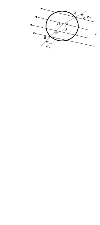
Figure 3: The neutrino incident angles at detectors $A$ and $B$, as measured individually from the local zenith, are given by $\psi_{\alpha}$ and $\psi_{\beta}$, respectively. The angle formed by $A$, $O$ (the Earth center), and $B$ is denoted as $\lambda$.

IV SN Neutrino Spectral Parameters and Multi-detector Analysis

In addition to the brief pulse of the neutronization $\nu_{e}$ burst, all three flavors of neutrinos and antineutrinos are emitted from the SN through pair production processes during a typical time scale $\sim 10$s. The primary SN neutrino spectrum, which is not pure thermal, is usually modeled as a pinched Fermi-Dirac distribution with several spectral parameters:

$$F^{0}_{i}\sim\frac{L_{i}}{T^{4}_{i}f_{3}(\eta_{i})}\frac{E^{2}}{e^{[(E/T_{i})-\eta_{i}]}+1},$$ (20)

where $L_{i}$ is the luminosity of the neutrino flavor $\nu_{i}$, $T_{i}$ is the effective temperature of $\nu_{i}$ inside the respective neutrinosphere, $E$ is the energy, $f_{3}(\eta_{i})$ is the normalization factor, and $\eta_{i}$ is the pinching parameter for $F^{0}_{i}$. Notice that $\eta_{\nu_{e}}\sim\eta_{\bar{\nu}_{e}}\sim\eta_{\nu_{x}}\sim 3.0$ is assumed here, where $\nu_{x}=\nu_{\mu}$, $\nu_{\tau}$, $\bar{\nu}_{\mu}$, and $\bar{\nu}_{\tau}$. The most significant difference between the Garching models (G1, G2) and the Lawrence Livermore model (LL) is that the Garching models exhibit a less hierarchical structure in the luminosity and in the average energy among different neutrino flavors, as shown in Table 2.

We assume a core collapse SN at a distance 10 kpc away. In a typical water Cherenkov detector, the isotropical inverse $\beta$-decay, $\bar{\nu}_{e}+p\rightarrow n+e^{+}$, is the most dominant process. In this work, other isotropical CC processes, $\nu_{e}+O\rightarrow F+e^{-}$ and $\bar{\nu}_{e}+O\rightarrow N+e^{+}$, are also included in the calculation. As for the directional events, we include the scattering events induced by $\nu_{i}$ and $\bar{\nu}_{e}$: $\nu_{i}(\bar{\nu}_{e})+e^{-}$, where $i=e,\mu,\tau$. The cross sections for $\bar{\nu}_{e}+p$ and $\nu_{i}(\bar{\nu}_{e})$ are adopted from Ref.cross-1 , and that for $\nu_{e}(\bar{\nu}_{e})+O$ are adopted from Ref.cross-2 . As shown in Fig. 3, the neutrino incident angle at a detector, denoted as $\psi_{\alpha}$ and $\psi_{\beta}$ for detector $A$ and $B$, respectively, may be defined as the angle measured from the local zenith. For a given $\psi_{\alpha}$, the allowed range for $\psi_{\beta}$ is limited. If the angle formed by $A$, the Earth center, and $B$ is given by $\lambda$, then

$$|\psi_{\alpha}-\lambda|<\psi_{\beta}<\psi_{\alpha}+\lambda$$ (21)

for $\psi_{\alpha}+\lambda<\pi$, and

$$|\psi_{\alpha}-\lambda|<\psi_{\beta}<2\pi-(\psi_{\alpha}+\lambda)$$ (22)

for $\pi<\psi_{\alpha}+\lambda<2\pi$. The density of Earth matter is of the order $\rho_{E}\sim 10g/cm^{3}$, and its variation is much smaller than that of the SN matter. One may adopt a simple step functionfreund as the approximation: $\rho_{E}\approx 5.0$ $g/cm^{3}$ for $\frac{1}{2}r_{\oplus}<r<r_{\oplus}$ (mantle), and $\rho_{E}\approx 12.0$ $g/cm^{3}$ for $r<\frac{1}{2}r_{\oplus}$ (core), where $r_{\oplus}$ is the Earth radius. For the purpose of illustration, one may analyze the expected results at two future detectors: the HyperKamiokandehk (detector $A$) and the MEMPHYSmemphys (detector $B$). The locations of the two detectors lead to $\lambda\sim\pi/2$.

Since the neutrino flux penetrates significant amount of Earth matter only when the incident angle at a detector is greater than $\pi/2$, no observable difference is expected from the two detectors if both $\psi_{\alpha}$ and $\psi_{\beta}$ are less than $\pi/2$. In this case, both $P_{2e}$ and $\bar{P}_{2e}$ reduce to $\sin^{2}\theta_{12}$, and all the observed differences between $A$ and $B$ vanish. Given the variety of spectral models, the present analysis is aiming at seeking for model-independent properties that would help identify the working scenario.

V Observables and Analyses

Figure 4: The ratio $\bar{D}^{(a)}$ as a function of the neutrino energy, with $\psi_{\alpha}=\pi/4$ (detector $A$ is unshadowed) and $\psi_{\beta}=0.95\pi$ (detector $B$ is shadowed by mantle and core). The primary neutrino spectra are adopted from G1, G2, and LL models.

Simultaneous observation of the SN neutrinos at two terrestrial detectors would yield the most useful results when pronounced Earth regeneration effect is observed at only one of the detectors. Given the two terrestrial detectors $A$ and $B$, a proper analysis of the expected neutrino event rates at the two detectors would in principle reveal the signatures representing distinct scenarios of the neutrino properties and mixing schemes. To pave the way for the analysis, we first examine the energy dependence of the relative flux difference at the detectors $A$ and $B$:

$$D=\frac{F^{B}_{\nu_{e}}-F^{A}_{\nu_{e}}}{F^{A}_{\nu_{e}}}$$ (23)

for the $\nu_{e}$ flux, and

$$\bar{D}=\frac{F^{B}_{\bar{\nu}_{e}}-F^{A}_{\bar{\nu}_{e}}}{F^{A}_{\bar{\nu}_{e}}}$$ (24)

for the $\bar{\nu}_{e}$ flux. With $F^{0}_{\nu_{i}}$ and $F^{0}_{\bar{\nu}_{i}}$ denoting the primary flux of $\nu_{i}$ and $\bar{\nu}_{i}$, respectively, one may relate the observed and the primary fluxes as

$$F_{\nu_{e}}=F^{0}_{\nu_{e}}+(1-P)(F^{0}_{\nu_{x}}-F^{0}_{\nu_{e}}),$$ (25)

$$F_{\bar{\nu}_{e}}=F^{0}_{\bar{\nu}_{e}}+(1-\bar{P})(F^{0}_{\bar{\nu}_{x}}-F^{0}_{\bar{\nu}_{e}}).$$ (26)

The three scenarios then lead to several distinct relative flux differences:

$$D^{(a)}=\frac{\sin^{2}\theta_{13}[F^{0}_{\nu_{e}}-F^{0}_{\nu_{x}}][P_{2e}-\sin^{2}\theta_{12}]}{F^{0}_{\nu_{e}}[\sin^{2}\theta_{13}\sin^{2}\theta_{12}]+F^{0}_{\nu_{x}}[1-\sin^{2}\theta_{13}\sin^{2}\theta_{12}]},$$ (27)

$$D^{(b)}=\frac{[F^{0}_{\nu_{e}}-F^{0}_{\nu_{x}}][P_{2e}-\sin^{2}\theta_{12}]}{F^{0}_{\nu_{e}}\sin^{2}\theta_{12}+F^{0}_{\nu_{x}}\cos^{2}\theta_{12}},$$ (28)

$$D^{(c)}=\frac{[F^{0}_{\nu_{e}}-F^{0}_{\nu_{x}}][P_{2e}-\sin^{2}\theta_{12}]}{F^{0}_{\nu_{e}}\sin^{2}\theta_{12}+F^{0}_{\nu_{x}}\cos^{2}\theta_{12}},$$ (29)

$$\bar{D}^{(a)}=\frac{-[F^{0}_{\bar{\nu}_{e}}-F^{0}_{\bar{\nu}_{x}}][\bar{P}_{2e}-\sin^{2}\theta_{12}]}{F^{0}_{\bar{\nu}_{e}}\cos^{2}\theta_{12}+F^{0}_{\bar{\nu}_{x}}\sin^{2}\theta_{12}},$$ (30)

$$\bar{D}^{(b)}=\frac{-\sin^{2}\theta_{13}[F^{0}_{\bar{\nu}_{e}}-F^{0}_{\bar{\nu}_{x}}][\bar{P}_{2e}-\sin^{2}\theta_{12}]}{F^{0}_{\bar{\nu}_{e}}[\sin^{2}\theta_{13}\cos^{2}\theta_{12}]+F^{0}_{\bar{\nu}_{x}}[1-\sin^{2}\theta_{13}\sin^{2}\theta_{12}]},$$ (31)

$$\bar{D}^{(c)}=\frac{-[F^{0}_{\bar{\nu}_{e}}-F^{0}_{\bar{\nu}_{x}}][\bar{P}_{2e}-\sin^{2}\theta_{12}]}{F^{0}_{\bar{\nu}_{e}}\cos^{2}\theta_{12}+F^{0}_{\bar{\nu}_{x}}\sin^{2}\theta_{12}}.$$ (32)

It is seen that the ratios also depend on the chosen model for the primary $\nu_{i}$ and $\bar{\nu}_{i}$ fluxes, as well as on $P_{2e}$ and $\bar{P}_{2e}$, which introduce the non-trivial energy dependence into $D$ and $\bar{D}$. As an illustration, we show the variation of $\bar{D}^{(a)}$ as a function of energy in Fig. 4, with $\psi_{\alpha}=\pi/4$ (detector $A$ is unshadowed) and $\psi_{\beta}=0.95\pi$ (detector $B$ is shadowed by mantle and core). The primary neutrino spectra are adopted from the G1, G2, and the LL models. Note that with the finite resolution power of the detector, not all the details of the curve can be observed in practice. It is clear from Eq.(30) that the energy dependence of $\bar{D}^{(a)}$ originates from the factor $\bar{P}_{2e}-\sin^{2}\theta_{12}$. The energy dependence of $D$ and $\bar{D}$, as shown in Eqs.(27-32), can be used to illustrate the properties of the observables that shall be proposed in this work.

Figure 5: The possible range of the value for $R=R(E)$ is indicated by the vertical range between two horizontal lines. Results for scenarios (a), (b), and (c) are shown here with the chosen bin size of 5 MeV. The incident angles $\psi_{\alpha}\leq\pi/2$ (detector $A$ unshadowed) and $\psi_{\beta}=0.95\pi$ (detector $B$ shadowed by mantle and core) are used to optimize the result. The estimated ranges of $R$ shown in the figures are determined by the results of the three spectral models and the statistical errors.

V.1 Relative difference of the event rates

In terms of the event rates, one may first examine the relative difference of the observed event rates per unit target mass for detectors $A$ and $B$:

$$R\equiv\frac{N_{B}-N_{A}}{N_{A}}.$$ (33)

The total event rates per unit target mass, $N_{A}$ and $N_{B}$, consist of all the isotropical and directional events mentioned in the previous section, with

$$N_{A,B}=\frac{\sum N_{i}}{M_{A,B}},$$ (34)

where $M_{A,B}$ denotes the total target mass of a detector. The expected event rates $N_{i}$ induced by the flavor $\nu_{i}$ (or $\bar{\nu}_{i}$) at the detector is given by

$$N_{i}=\frac{N_{t}}{4\pi L^{2}}\int[\sum_{y}F_{\nu_{i}}\times\sigma_{iy}]dE,$$ (35)

where $N_{t}$ is the target number at the detector, $L$ is the distance to the supernova, $\sigma_{iy}$ is the cross section for $\nu_{i}$ (or $\bar{\nu}_{i}$) in a particular reaction channel $y$. The detection efficiency is assumed to be one. In the following, one may denote the resultant values of $R$ for the six scenarios as $R^{J}$, where $J=(a),(b)$, $(c)$.

As an illustration, we show in Fig. 5 the expected values of $R$ for scenarios $(a)$, $(b)$, and $(c)$. The reasonable estimation of the energy bin size is roughly a few MeV for the detection of typical SN neutrinosfogli:jcap05 . We adopt an energy bin size of 5 MeV in the figure. Note that for scenario $(b)$, the deviation of $R$ from zero is $\sim 1\%$ or smaller, and the sign of $R$ is undetermined with the error bar. The estimated width for $R$ is given by the different results from the three spectral models and the statistical errors from each. As an example, one notes that the expected values of $R^{(a)}$ under LL, G1, and G2 models in 25 MeV $<E<$30 MeV are estimated to be $-0.085\pm 0.057$, $-0.221\pm 0.112$, and $-0.216\pm 0.109$, respectively. The resultant $R^{(a)}$ is then shown in Fig. 5 with the combined width $-0.333<R^{(a)}<-0.027$ for 25 MeV $<E<$30 MeV. Note that there is no apparent energy dependence of the width.

Even though some details of the energy-dependence in Fig. 5 are lost, certain useful qualitative properties are still available. It is seen that the Earth effect could suppress the event rates to an observable level (of order 10% or more) for $E\geq 25$ MeV if the working scenario is $(a)$ or $(c)$. The sign and the magnitude of $R$ in $E\geq 25$ MeV can be used to separate the three scenarios into two groups: $[(a),(c)]$ and $(b)$. It should be pointed out that for $E<25$ MeV, the uncertainties wipe out the small deviation from zero and the sign of $R$ is undetermined for all scenarios.

Figure 6: The values of $S=S(E)$ estimated with the bin size of 5 MeV and $\psi_{\alpha}\leq\pi/2$ (detector $A$ unshadowed), $\psi_{\beta}=0.95\pi$ (detector $B$ shadowed by mantle and core). The ranges of $S$ shown in the figure are based on the combined results of the three spectral models and the statistical errors.

More hints may be available from analyzing the directional events alone, which are predominantly the $\nu_{e}$-induced elastic scattering events. However, the directional event rate is approximately $1\sim 2$ orders of magnitude less than the isotropical event rate. Extracting the directional events effectively from the dominant background of the isotropical events may be quite challenging in practice. In the following analysis, one assumes that the directional event rates in the forward cone with a narrow solid angle can be identified.

V.2 Relative difference of the directional events

We may define another ratio based on the directional events per unit mass of target at the two detectors,

$$S\equiv\frac{n_{B}-n_{A}}{n_{A}},$$ (36)

where $n_{B}$ and $n_{A}$ denote the shadowed and the unshadowed directional events per unit target mass, respectively. The properties of $S$, as shown in Fig. 6, lead to new information that is unseen from $R$. One notes that two groups of scenarios, $(a)$ and $[(b),(c)]$, could be identified by the magnitude of $S$ at the high energy end since the magnitude could differ by a factor of three or more. Thus, one may conclude that the degeneracy between $R^{(a)}$ and $R^{(c)}$ could be removed by using the observable $S$, and that the three scenarios could be reasonably distinguished by analyzing both $R$ and $S$ at the high energy end.

It should be pointed out that even though $R$ and $S$ represent energy-integrated quantities, they still exhibit general energy dependence with the chosen finite bin size, as can be seen from Figs. 5 and 6. To qualitatively illustrate this general properties, one may approximate $R$, for simplicity, as the event ratios that consist only of the predominant $\bar{\nu}_{e}+p$ events. For scenario $(a)$, Eqs.(25-26) and (33-35) lead to

$$R^{(a)}\simeq\frac{[F^{0}_{\bar{\nu}_{e}}-F^{0}_{\bar{\nu}_{x}}]\int(\bar{P}_{2e}-\sin^{2}\theta_{12})\sigma(E)dE}{\int(F^{0}_{\bar{\nu}_{e}}\cos^{2}\theta_{12}+F^{0}_{\bar{\nu}_{x}}\sin^{2}\theta_{12})\sigma(E)dE},$$ (37)

where $\sigma(E)$ is the cross section. With the input parameters and a given model for the fluxes,

$$R^{(a)}\sim\frac{\int(\bar{P}_{2e}-\sin^{2}\theta_{12})\sigma(E)dE}{\int\sigma(E)dE}.$$ (38)

If one calculates $R^{(a)}$ in a relative small step in energy, $\Delta E\sim$ a few MeV, the cross section $\sigma=\sigma(E)$, which is roughly $\sigma\sim E^{2}$, would be relatively smooth as compared to the function $\bar{P}_{2e}$. As a consequence, one may expect $R^{(a)}\sim\bar{P}_{2e}-\sin^{2}\theta_{12}$. It is seen from Eq.(30) that the qualitative behavior of the factor, $\bar{P}_{2e}-\sin^{2}\theta_{12}$, which dictates the general trend of the energy dependence of $\bar{D}^{(a)}$ in Fig. 4, propagates to $R^{(a)}$ in Fig. 5. The energy dependence of $S$, and that of $T$, which is introduced in the next subsection, can be realized in a similar way.

V.3 Double ratio with both directional and isotropical events

The observables, $R$ and $S$, tend to flip signs near the peak of the spectrum ($\sim 25$ MeV), and become less useful for analyzing the abundant events induced by the neutrinos with energies near the peak. It would be worth while to further investigate whether there is more to learn from the middle range of the spectrum. Theoretically, the Earth regeneration effect is signaled by the oscillatory modulations of the observed spectra. A quantitative analysis of the resultant event rates, however, may be quite subtle. The resolution power of the detector is limited and the modulation may not alter the total event rates significantly enough to render an observable difference between the shadowed and the unshadowed events. To optimize the results for an analysis, neutrino event rates from a specific range of energy cut may be needed.

Figure 7: The possible ranges of $T=T(\psi_{\beta})$ for scenarios $(a)$, $(b)$, and $(c)$ are estimated from the combined results of the three spectral models and the statistical errors for $15<E<30$ MeV. The incident angle for detector $A$ is chosen as $\psi_{\alpha}=\pi/2$, and an assumed directional resolution of $\pi/12$ for detector $B$ is adopted. The resultant range of $T$ in each scenario is expected to show no $\psi_{\beta}$-dependence for $\psi_{\beta}\leq\pi/2$.

One may construct a double ratio with both the isotropical and the directional events:

$$T\equiv\frac{[(N_{B}-n_{B})-(N_{A}-n_{A})]/(N_{A}-n_{A})}{(n_{B}-n_{A})/n_{A}},$$ (39)

where $N-n$ and $n$ denote the isotropical and the directional events, respectively. Depending on the time of a day, a given incident angle $\psi_{\alpha}$ for detector $A$ corresponds to a definite incident angle $\psi_{\beta}$ for detector $B$. Notice that the possible values of $\psi_{\beta}$ are regulated by Eqs. (21) and (22). If $\psi_{\alpha}\sim 0$ or $\psi_{\alpha}\sim\pi$, the angle $\psi_{\beta}$ is limited to a narrow range: $\psi_{\beta}\sim\lambda\sim\pi/2$. On the other hand if $\psi_{\alpha}\sim\pi/2$, the allowed range for $\psi_{\beta}$ becomes maximized: $0<\psi_{\beta}<\pi$, and the observables are expected to vary with a wide range of $\psi_{\beta}$. Each of the two detectors may be unshadowed (if $\psi_{\alpha,\beta}<\pi/2$), shadowed by the mantle (if $\pi/2<\psi_{\alpha,\beta}<5\pi/6$), or shadowed by the mantle and the core (if $5\pi/6<\psi_{\alpha,\beta}<\pi$). In any case, more useful hints from a simultaneous observation would be available if one of the incident angles is greater than $\pi/2$ and the other is less that $\pi/2$.

The observable $T$ may be used as a supplementary tool to the other two observables, $R$ and $S$. As an illustration, the ratio $T$ is evaluated here for $15<E<30$ MeV and analyzed as a function of $\psi_{\beta}$, with $\psi_{\alpha}=\pi/2$ and a conservatively assumed directional resolution of $\pi/12$ for detector $B$, as shown in Fig. 7. Notice that the pointing accuracy of the incident neutrinos at the SK detector can reach the level to within a few degrees at 10 kpc tomas:03 . The results for each scenario are expected to show no $\psi_{\beta}$-dependence for $\psi_{\beta}\leq\pi/2$. In addition, calculations show that scenarios $(b)$ leads to small deviations from zero: $-0.078<T<0.076$, which can be distinguished from the other two scenarios. Furthermore, $T^{(a)}$ and $T^{(c)}$ can also be distinguished by the difference in magnitude. One would expect that a combined analysis of $R$, $S$, and $T$ should be able to provide certain useful constraint or prediction about the neutrino parameters.

VI Summary and Conclusions

The SN neutrino burst has long been considered as a promising tool for probing the neutrino mass hierarchy and the mixing angle $\theta_{13}$. The current consensus is that the contributions from both the MSW and the non-MSW effects should be included in analyzing the flavor transition of the SN neutrino signals. However, the uncertain local density profile of the SN matter and the neutrino spectral parameters may lead to diverse interpretations to the neutrino signals from the contribution of the MSW effect. To investigate the consequences resulting from these uncertainties, this work suggests a more general parametrization for the uncertain local density profile, and outlines a scheme using ratios of experimental observables as the discriminators for the possible scenarios that are related to the MSW effect. As an illustration, we analyze the expected event rates at two terrestrial Cherenkov detectors. The consequences due to choices of the existing spectral models are included in the analysis. The possible scenarios arising from the uncertainties are then examined through the observables $R$, $S$, and $T$. It is seen that the uncertain local density profile of the SN matter can alter the predictions for $\theta_{13}$ and the mass hierarchy from the contribution of the MSW effect alone. The predicted bound for $\theta_{13}$ is regulated by the proposed function $g(n_{h},\theta_{13})$.

The results in this work are derived from the expected event rates at two megaton-scale Cherenkov detectors that would be available in the future. Analyses of the future SN neutrinos based on other types of detectors, such as the liquid Argon and kton-scale scintillation detectors that are sensitive to distinct channels of the neutrino interactions, should also provide valuable information toward a better understanding of the neutrino parameters and the SN physics. A detailed analysis based on all the three types of detector is performed in, $e.g.$, Ref. 6, in which seven SN and neutrino parameters are taken into consideration. To extend the present work, it would be intriguing to investigate how the uncertain density profile would impact the outcome of the analysis based on the detectors other than the Cherenkov ones.

In shaping a possible new paradigm for the neutrino flavor conversion in a SN, recent studies and simulations suggest that the shock wave propagation and certain types of non-MSW flavor conversion may occur in the complex environment of a SN at different space and time scales if the proper physical conditions are met. These effects, such as the neutrino self coupling in dense mediaraffelt:07 ; dd:08 ; flmm:08 ; fq:06 ; hr:06 ; df:06 ; pr:02 ; rs:07 ; ad:08 ; ddm:08 and the neutrino flavor de-polarization associated with the after shock turbulencebenatti:95 ; fg:06 ; mon:06 ; chou:07 , may have different origins from that of the MSW effect and would impact the efficiency of neutrino flavor transition.

It is suggested that the neutrino self interactions induce collective flavor transitions, which may occur before or in the same region as the resonant flavor transition. The size of modification to the original neutrino flux depends on the mass hierarchy, as well as on the mixing angle $\theta_{13}$. As an example, one considers the simplest case when the self-interaction effects can be factored out from the ordinary MSW effects. For the inverted hierarchy, it is suggested that if $\theta_{13}$ is nonzero, the collective pair-conversion of the type $\nu_{e}\bar{\nu}_{e}\rightarrow\nu_{x}\bar{\nu}_{x}$ can be triggered before the ordinary MSW effect occurslisi:07 . Thus, even in the simplest case, the altered primary spectra could impact the validity and the usefulness of the observables proposed in this work. A better understanding of the modified neutrino spectra resulting from the collective effects would help in establishing more convenient and useful observables since the knowledge of the neutrino spectra before and after the MSW effect is essential for the present analysis. Note that the treatment of the variable density profile for the MSW effect, as that proposed in this work, is unaffected by the non-MSW effects.

The shock wave propagation, on the other hand, may alter the density profile of the SN matter and induce certain non-linear effects that modify the neutrino survival probabilities and the neutrino spectrum. In particular, there is a possibility that more than one MSW-resonance related to the same scale of mass-squared difference could arise due to the shock wave propagation. The effects of the shock wave on certain physical observables, with the emphasis on the time-dependent properties, are analyzedGa ; fogli:jcap05 ; sf . Although the proposed scheme in the present work is limited to the discussion without considering specific scenario due to the shock effects, it takes into account the possible varying density profile, and is not limited to whether the profile is actually primary. In addition, the quantities $R$, $S$, and $T$ are proposed in this work to examine the time-integrated behaviors of the event rates. As an extension to this present analysis, it would be intriguing to further investigate weather the time structure of the shock waves effects and the possible multiple MSW-resonance due to the shock effect can alter the time-integrated properties of the proposed quantities to an observable level. Even with the unknown neutrino parameters, the uncertain model for the SN neutrino spectrum, and the possible statistical errors, the quantities $R$, $S$, and $T$ might still be able to provide another potential means for probing the SN physics if they reveal time-independent signatures that are related to the shock wave propagation. On the other hand, if the shock signatures are unobservable with these time-integrated quantities, then these quantities might be able to provide insights to the neutrino parameters without being affected by the shock waves.

It should be emphasized that the present work is devoted to effects that are related to the MSW resonant flavor transition in a SN. The focus is aimed at the possible modification to the results of MSW effect due to the uncertain density profile. This modification is expected to have certain impact to the complete analysis based on both the MSW effect and the non-MSW effects. The whole details of the non-MSW effects, as well as the interplay between the MSW and the non-MSW consequences, are still not fully understood. The neutrino flavor conversion in a SN remains as a complicated problem that awaits for more complete answers. Whether the flavor transition arising from one origin would dominate over that from the others depends on the uncertain spectral parameters, the undetermined neutrino intrinsic properties, and the physical conditions that the neutrinos encounter at different stages of the SN environment. In addition, the reliability of the analysis relies on whether the MSW and non-MSW effects can be analyzed separately. However, these unrelated types of effects decouple only when specific physical conditions are met.

In any case, analysis of the non-trivial MSW flavor conversion due to the possible drastic variation of the local density profile, as discussed in this work, should provide certain insight in probing the neutrino parameters and in shaping a more convincing paradigm for the neutrino flavor conversion in the SN.

- (1) A. S. Dighe and A. Yu. Smirnov, Phys. Rev. D 62, 033007 (2000).
- (2) C. Lunardini and A. Yu. Smirnov, JCAP 0306, 009 (2003).
- (3) V. Barger, D. Marfatia, and B. P. Wood, Phys. Lett. B 547, 37-42 (2002).
- (4) H. Davoudiasl and P. Huber, Phys. Rev. Lett. 95, 191302 (2005).
- (5) G. L. Fogli, E. Lisi, D. Montanino, and A. Palazzo, Phys. Rev. D 65, 073008 (2002).
- (6) S. Skadhauge and R. Z. Funchal, JCAP 0704, 014 (2007).
- (7) M. Kachelriess and R. Tomas, arXiv:hep-ph/0412100.
- (8) C. Lunardini and A. Yu. Smirnov, Nucl. Phys. B 616, 307 (2001).
- (9) A. Mirizzi, G. G. Raffelt and P. D. Serpico, JCAP 0605, 012 (2006).
- (10) A. S. Dighe, M. T. Keil, and G. G. Raffelt, JCAP 0306, 005 (2003).
- (11) H. Minakata, H. Nunokawa, R. Tomas, and J. W. F. Valle, JCAP 0812, 006 (2008).
- (12) S. Skadhauge and R. Z. Funchal, arXiv:hep-ph/0802.1177 (2008).
- (13) S. H. Chiu and T. K. Kuo, Phys. Rev. D 73, 033007 (2006).
- (14) S. H. Chiu, Phys. Rev. D 76, 045004 (2007).
- (15) R. Tomas, M. Kachelriess, G. G. Raffelt, A. Dighe, H. T. Janka and L. Scheck, JCAP 0409, 015 (2004).
- (16) R. Buras, H. T. Janka, M. T. Keil, G. G. Raffelt and M. Rampp, Astrophys. J. 587, 320 (2003).
- (17) K. Takahashi, M. Watanabe, K. Sato, and T. Totani, Phys. Rev. D 64, 093004 (2001).
- (18) T. K. Kuo and J. Pantaleone, Phys. Rev. D 37, 298 (1988).
- (19) S. E. Woosley and T. A. Weaver, Astrophys. J. Suppl. Ser. 101, 181 (1995).
- (20) S. E. Woosley, A. Heger, and T. A. Weaver, Rev. Mod. Phys. 74, 1015 (2002).
- (21) Shin’ichiro Ando and Katsuhiko Sato, JCAP 0310, 001 (2003).
- (22) T. K. Kuo and J. Pantaleone, Rev. Mod. Phys 61, 937 (1989).
- (23) A. N. Ioannisian and A. Yu. Smirnov, Phys. Rev. Lett. 93, 241801 (2004).
- (24) A. N. Ioannisian, N. A. Kazarian, A. Yu. Smirnov, and D. Wyler, Phys. Rev. D 71, 033006 (2005).
- (25) J. Arafune and M. Fukugita, Phys. Rev. Lett. 59, 367 (1987).
- (26) W. Haxton, Phys. Rev. D 59, 2283 (1987).
- (27) M. Freund and T, Ohlsson, Mod. Phys. Lett. A 15, 867 (2000).
- (28) K. Nakamura, Int. J. Mod. Phys. A18, 4053-4063 (2003)
- (29) A. de Bellefon et al., hep-ex/0607026.
- (30) G. L. Fogli, E. Lisi, A. Mirizzi, and D. Montanino, JCAP 0504, 002 (2005).
- (31) R. Tomas, D. Semikoz, G. G. Raffelt, M. Kachelriess, and A. S. Dighe, Phys. Rev. D 68, 093013 (2003).
- (32) G. G. Raffelt, arXiv:astro-ph/0701677.
- (33) B. Dasgupta and A. Dighe, Phys. Rev. D 77, 113002 (2008).
- (34) G. Fogli, E. Lisi, A. Marrone, and A. Mirizzi, arXiv:hep-ph/0805.2530 (2008).
- (35) G. M. Fuller and Y.-Z. Qian, Phys. Rev. D 73, 023004 (2006).
- (36) S. Hannestad, G. G. Raffelt, G. Sigl, and Y. Y Wong, Phys. Rev. D 74, 105010 (2006).
- (37) H. Duan, G. M. Fuller, and Y.-Z. Qian, Phys. Rev. D 74, 123004 (2006).
- (38) S. Pastor and G. Raffelt, Phys. Rev. Lett. 89, 191101 (2002).
- (39) G. G. Raffelt and A. Y. Smirnov, Phys. Rev D 76, 081301 (2007).
- (40) Amol Dighe, AIP Conf. Proc. 981, 75-79 (2008).
- (41) B. Dasgupta, A. Dighe, and A. Mirizzi, Phys. Rev. Lett. 101, 171801 (2008).
- (42) F. Benatti and R. Floreanini, Phys. Rev. D 71, 013003 (2005).
- (43) A. Friedland and A. Gruzinov, arXiv:astro-ph/0607244 (2006).
- (44) G. Fogli, E. Lisi, A. Mirizzi, and D. Montanino, JCAP 0606, 012 (2006).
- (45) S. Choubey, N. P. Harries, and G. G. Ross, Phys. Rev. D 76, 073013 (2007).
- (46) G. L. Fogli, E. Lisi, A. Marrone, and A. Mirizzi, JCAP 0712, 010 (2007).
- (47) R. C. Schirato and G. M. Fuller, arXiv:astro-ph/0205390 (2002).