Nonsensitive nonlinear homotopy approach

Abstract

Generally, natural scientific problems are so complicated that one has to establish some effective perturbation or nonperturbation theories with respect to some associated ideal models. In this Letter, a new theory that combines perturbation and nonperturbation is constructed. An artificial nonlinear homotopy parameter plays the role of a perturbation parameter, while other artificial nonlinear parameters, of which the original problems are independent, introduced in the nonlinear homotopy models are nonperturbatively determined by means of a principle minimal sensitivity. The method is demonstrated through several quantum anharmonic oscillators and a non-hermitian parity-time symmetric Hamiltonian system. In fact, the framework of the theory is rather general that can be applied to a broad range of natural phenomena. Possible applications to condensed matter physics, matter wave systems, and nonlinear optics are briefly discussed.

In general, natural scientific problems cannot be exactly described by some analytical expressions. What scientists usually do is just first to establish some ideal models, and then to consider additional effects by use of some perturbation and nonperturbation theories.

Perturbation theories (PTs) YangJK ; Ablowitz already have quite a long and interesting history in physics. They have been used to explore physical systems that can not be solved exactly but with a small parameter. Though great challenges are coming from the blooming numerical calculation methods, PTs are still showing their great power in solving various problems. For instance, perturbation theories have been used to study the spectrum of non-hermitian parity-time ($\mathcal{PT}$) symmetric Hamiltonian PTS , the structure of trapped Bose-Einstein condensates (BECs) with long-range anisotropic dipolar interactions dBEC , and the interacting fermions in two-dimensions Fermion . Besides, the fundamental ideas of PTs have been utilized to study some models in quantum computation theory (QCT). Techniques based on PTs have also been applied to engineer interesting Hamiltonians, whereby the outstanding perturbation theory gadgets (PTGs) technique was developed MB1 ; MB2 . A short but incisive review of the history of PT and its new development in quantum many-body theory, quantum computation and quantum complexity theory has been given recently by M. M. Wolf Wolf .

On the other hand, nonperturbation theories (NPTs) have been established to solve real scientific problems with the lack of a small parameter that acts as a perturbation parameter. In this case, some parameters will be artificially introduced as some formal perturbation parameters and/or nonperturbation parameters. Usually, one of these artificial perturbation parameters have to be set finite, say, the unit one, while others will be determined in some nonperturbative ways such as some types of optimized approaches.

Considering the fact that physical quantities should be independent of any particular perturbation and/or nonperturbation method used to calculate them, Stevenson 1981 proposed an optimized perturbation theory (OPT) with the principle of minimal sensitivity (PMS) as a key ingredient. Some other perturbation methods appeared in 1970’s and 1980’s, such as the non-parameter expansion method 1979 , and the linear $\delta$ expansion method (LDE) 8788 ; 1990 ; LuWF ; 2005 ; 1993 ; 1993a ; 1995 , have the same idea as implied in the OPT. These methods, especially the LDE, have found successful applications in many physical contexts during the past three decades.

Actually, as we will show later in this Letter, the basic idea underlying those methods mentioned above can be integrated into a general framework of the (linear) homotopy analysis method (HAM) kowalski ; liao . In the language of field theory, it is possible to construct a new action $S_{q}=\mathcal{H}(S_{0},S,q)$ by building a homotopy relation between an original action $S$ and a trial ideal action $S_{0}$ (which is solvable and reflects as much as possible physics of $S$). Here $S$ can represent any object or quantity for any scientific problem, such as the Green function, density operator, distribution function, generating functional, differential equations, and so on. $q\in[0,1]$ is called a homotopy parameter. $S_{q}$ is fixed at the two endpoints, i.e., $S_{q=0}=S_{0}$ and $S_{q=1}=S$, while can possess different expressions when $q\neq 0,1$, depending on $\mathcal{H}(S_{0},S,q)$. Hence, different homotopy relations yield different actions. For example, a linear homotopy relation yields an action as $S_{q}=(1-q)S_{0}+qS$, which is exactly the form used in the LDE and other methods mentioned above. However, the homotopy relation is by no means constrained to be linear. We can introduce a simple and direct nonlinear extension

$$S_{q} = (1-q)S_{0}+\sum_{i=1}^{n}q^{i}S_{i}+q^{n+1}\left(S-\sum_{i=1}^{n}S_{i}\right).$$ (1)

In the standard procedure of the LDE, $S_{0}$ contains one or more auxiliary parameters $\eta_{i}$. In our generalized nonlinear homotopy relation (1), auxiliary actions $S_{1},S_{2},\ldots,S_{n}$ also contain some parameters $\xi_{i}$. These parameters are also artificial, which means that $S_{q=1}=S$ is independent of both $\eta_{i}$ and $\xi_{i}$. This can be easily verified with the help of Eq. (1), as all $S_{i}~{}(i=1\ldots n)$ will be eliminated when the nonlinear homotopy parameter $q$ is set to 1. In order to describe it more explicit and without losing the nonlinear property of Eq. (1), let us throw away $O(q^{3})$ terms to obtain

$$S_{q} = (1-q)S_{0}(\eta)+qS_{1}(\xi)+q^{2}(S-S_{1}(\xi)),$$ (2)

with only two auxiliary parameters $\eta$ and $\xi$. Any desired physical quantity $\Phi$ can be evaluated as a perturbation series of $q$, which is set equal to 1 at the final step. If the series is truncated at $q^{N},N\geq n+1=2$, the approximant $\Phi^{(N)}$ is obviously dependent of $\eta$ and $\xi$, while it will have no relation with those two auxiliary parameters when $N\rightarrow\infty$. In practice, $N$ is always finite, it is therefore necessary to choose these parameters nonperturbatively to make the expansion reasonable. We will take the PMS as an effective criterion. According to the PMS, the auxiliary parameters $\eta$ and $\xi$ should be selected to minimize the sensitivity of the perturbation expansion to some small variations in them. It is remarkable that a nonlinear homotopy relation and the combination of the perturbation and nonperturbation theories via the PMS are two fundamental ingredients of our nonsensitive nonlinear homotopy approach (NNHA).

Before moving to concrete examples, let us discuss a little more about the PMS. There is a natural way to fix the parameters $\xi$ and $\eta$, which is to solve the following equation system

$$\frac{\partial\Phi^{(N)}(\eta,\xi)}{\partial\eta}=0,\quad\frac{\partial\Phi^{(N)}(\eta,\xi)}{\partial\xi}=0$$ (3)

similar to the usual OPT theory. However, the above system does not always have one solution. Eqs. (3) might have many solutions $\{\xi_{i},\eta_{i}\}$, therefore, we have to find a method to fix one of them according to the PMS. To this end, we define the $M$-th sensitivity $\kappa^{(N)}_{M}$

$$\kappa^{(N)}_{M}=\sum_{j=1}^{M}\left\|\frac{\textrm{d}^{M}\Phi^{(N)}}{\textrm{d}\xi^{j}\textrm{d}\eta^{M-j}}\right\|,$$ (4)

where $\|\cdot\|$ denotes the norm. It is clear that the sensitivities $\kappa^{(N)}_{M}$ for all $M$ should tend to zero as $N\rightarrow\infty$, because the real model is $\{\xi,\eta\}$ independent. Consequently, it is natural to pick out the final required $\{\xi,\eta\}$ by minimizing the first few sensitivities $\kappa^{(N)}_{i}(i=1,2,...,k)$ for the smallest $k$. More details can be seen in the following concrete examples. It is clear that a solution (if it exists) of Eqs. (3) is really a minimum of the first sensitivity (FS) $\kappa^{(N)}_{1}$.

Now we use our theory to study an eigenvalue problem of a given Hamiltonian. This is a basic problem included in almost all quantum physical problems. For instance, various models in condensed matter physics deal with ground-states of spin Hamiltonians, and quantum computation can be performed by encoding a solution of a computation problem into the ground-state of a Hamiltonian Wolf . The calculation of energy levels for a Hamiltonian system is also a crucial problem in solid physics Fermion . As the first example, we apply the theory to calculate the ground-state energy of a sextic quantum anharmonic oscillator

$$H=p^{2}+x^{2}+x^{6}.$$ (5)

Generally, through a nonlinear homotopy relation in the form of Eq. (2), we can construct a new Hamiltonian

$$H_{q}=(1-q)(H_{0})+q(H_{1})+q^{2}(H-H_{1}).$$ (6)

Here we choose $H_{0}=p^{2}+\omega x^{2}$ and $H_{1}=p^{2}+x^{2}+\lambda x^{6}$, and thus obtain

$$H(q,\omega,\lambda) = (1-q)(p^{2}+\omega x^{2})+q(p^{2}+x^{2}+\lambda x^{6})$$ (7)

$$+q^{2}(1-\lambda)x^{6}.$$

It is obvious that $H_{0}$ is the Hamiltonian of a harmonic oscillator with an auxiliary parameter $\omega$ denoting the frequency of the oscillation. $H_{1}$ is a new term which can not be included without the second order term of $q$. It is an auxiliary Hamiltonian with a parameter $\lambda$ denoting the intensity of an additional sextic effect. It is easy to verify that $H(1,\omega,\alpha)=H$, and $H(0,\omega,\alpha)=H_{0}$.

Making advantage of Bender and Wu’s work Wu , we obtain the ground-state energy of $H(q,\omega,\alpha)$ as a power series of $q$,

$$E_{HT}(q,\omega,\lambda)=\omega-\frac{(15\lambda-4\omega^{4}+4\omega^{2})}{8\omega^{3}}q+\ldots,$$ (8)

which can be easily calculated to any order of $q$, with the help of the symbolic calculation softwares. Using MAPLE, we calculate the series up to order 21, and obtain an analytical expression of the approximate ground-state energy $E^{(21)}_{HT}(q,\omega,\lambda)$, and finally set $q=1$.

Now comes the problem to determine parameters $\omega$ and $\lambda$ under the PMS. Roughly speaking, the PMS tends to pick out parameters around which the profile of $E^{(21)}_{HT}(1,\omega,\lambda)$ is the “flattest”. So what can be learned from the profile of $E^{(21)}_{HT}$ as displayed Fig. 1, where the symbolic $E$ denotes $E^{(21)}_{HT}$? It is discovered that when $(\omega,\lambda)$ varies in the region $[3.7,4]\times[0.25,0.4]$, the variation in the energy $E^{(21)}_{HT}$ is less than $10^{-6}$. We take a very accurate value $E_{ex}=1.435\ 624\ 619$ as an “exact” result, which is given by Meißner and Steinborn exact . Thus we have an error $E^{(21)}_{HT}-E_{ex}$ vary from $-4.62\times 10^{-6}$ to $5.38\times 10^{-6}$ in the above region. In the case that the exact value of a solution is not known, we can calculate $E^{(21)}_{HT}-E^{(20)}_{HT}$ as an error. It is reasonably found that $E^{(21)}_{HT}-E^{(20)}_{HT}\sim 10^{-6}$. To pick out an optimal point in this region, let us go further from the figure to determine a pair of nonsensitive parameters numerically. In Fig. 2 we draw the curves of $\frac{\partial E^{(21)}_{HT}}{\partial\omega}=0$ (solid) and $\frac{\partial E^{(21)}_{HT}}{\partial\lambda}=0$ (dash), and find that they do not intersect in this region. In this situation, we can not obtain a pair of $(\omega,\lambda)$ to vanish these two first-order partial derivatives simultaneously. Motivated by the spirit of the PMS, we minimize the FS for $\Phi^{(N)}=E^{(21)}_{HT}(\omega,\lambda)$ by simply taking the norm as $\|A\|=A^{2}$. Consequently, a pair of parameters $\omega=3.847\ 166$ and $\lambda=0.377\ 585$ is obtained to minimize the FS. The substitution of these parameters into the approximant $E^{(21)}_{HT}(1,\omega,\lambda)$ leads to an approximate energy $E^{(21)}_{HT}=1.435\ 624$ with an error of $-5.53\times 10^{-7}$.

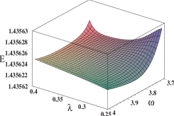
Figure 1: $E^{(21)}_{HT}$ as a function of $\omega$ and $\lambda$ in the region $[3.7,4]\times[0.25,0.4]$.

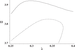
Figure 2: The curves of $\frac{\partial E^{(21)}_{HT}}{\partial\omega}=0$ (solid) and $\frac{\partial E^{(21)}_{HT}}{\partial\lambda}=0$ (dash).

As a compare, we also give an approximant truncated at order 21 for the ground-state energy by using a linear homotopy relation as $H(q,\omega)=(1-q)(p^{2}+\omega x^{2})+q(p^{2}+x^{2}+x^{6})$, which has been applied in the LDE method. It yields an approximant $E^{(21)}_{LDE}(q,\omega)$ which only depends on $\omega$, after $q$ is set to be 1. After some similar procedures, we obtain a final result $E^{(21)}_{LDE}(1,\omega_{0})=1.435\ 428$ with $\omega_{0}=5.254\ 070$ satisfying ${\textrm{d}E^{(N)}}/{\textrm{d}\omega}=0$. The error of $E^{(21)}_{LDE}$ is $-1.97\times 10^{-4}$, which is about $10^{3}$ times larger than that of $E^{(21)}_{HT}$. The above example and the corresponding numerical results show that our theory does largely improve the accuracy of the approximant without more difficulty. We have also study the ground and excited states for some quartic and octic anharmonic oscillators in the same way, and drawn the same conclusions. It is remarkable that when the coefficients of the anharmonic terms are large, the method is still applicable and the accuracy is at the same level.

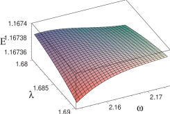
Figure 3: $E^{\prime(21)}_{HT}$ as a function of $\omega$ and $\lambda$ in the region $[1.68,1.69]\times[2.153,2.175]$.

Next we go further to study non-hermitian Hamiltonian systems. Recently, many progresses have been made for non-hermitian $\mathcal{PT}$-symmetric physics. We are thus motivated to investigate the energy spectrum of a non-hermitian Hamiltonian with $\mathcal{PT}$-symmetry. Bender and his co-workers have demonstrated that such a $\mathcal{PT}$-symmetric Hamiltonian

$$H^{\prime}=p^{2}+\frac{1}{4}x^{2}+ix^{3},$$ (9)

has a real and positive spectrum Bender . According to our theory, the nonlinear homotopy relation can also be built to link a non-hermitian Hamiltonian with some auxiliary Hamiltonians that can be either hermitian or non-hermitian. For instance, a nonlinear homotopy Hamiltonian can be constructed as

$$H^{\prime}(q,\omega,\lambda) = (1-q)(p^{2}+\omega x^{2})+q(p^{2}+\frac{1}{4}x^{2}+i\lambda x^{3})$$ (10)

$$+iq^{2}(1-\lambda)x^{3}.$$

It can be seen that $H^{\prime}(q,\omega,\lambda)$ also has the $\mathcal{PT}$-symmetry, and its ground-state eigenvalue can be expressed as

$$E^{\prime}_{HT}(q,\omega,\lambda)=\omega+\frac{1-4\omega^{2}}{8\omega}q+\ldots,$$ (11)

where the coefficients of each order of $q$ are real. Truncating the series at order 21 and setting $q=1$ yield an approximant $E^{\prime(21)}_{HT}$ for the ground-state energy of $H^{\prime}$. The pair that eliminates the FS (4) for $\Phi^{(N)}=E^{\prime(21)}_{HT}(\omega,\lambda)$ is $\{\omega=2.160\ 887,\lambda=1.684\ 022\}$, and the profile of $E^{\prime(21)}_{HT}$ around this stationary point is shown in Fig. 3 with $E$ denoting $E^{\prime(21)}_{HT}$. At the stationary point, $E^{\prime(21)}_{HT}$ equals $1.167\ 384$, with an error $7.61\times 10^{-5}$ compared with the numerical result $1.167\ 46$ given by Bender and Dunne JMP .

This example reveals great validity of our theory on investigating non-hermitian $\mathcal{PT}$-symmetric Hamiltonian systems. Besides, our theory can be used to study more complicated problems beyond a linear eigenvalue problem. It is shown in a series of recent works that nonlinear localized structures can be generated in $\mathcal{PT}$ periodic potentials soliton-pt ; beam . Optical solitons are produced by adding a self-focusing Kerr nonlinear $\mathcal{PT}$-symmetric potential $iW(x)$, which satisfies $W(-x)=-W(x)$, to the usual nonlinear Schrödinger equation. Our theory can also be applied to investigate this type of nonlinear $\mathcal{PT}$-symmetric system by building suitable homotopy relations associating a system hard to be exactly solved with those solvable. In this way, the knowledge of the latter can be used to explore the original system approximately, and the necessary accuracy is entirely ensured by the principle of minimal sensitivity.

As is known, physical models that can be solved exactly are very rare. In a recent work on the structure of trapped Bose-Einstein condensates (BECs) with long-range anisotropic dipolar interactions, it is found that a small perturbation in the trapping potential can lead to dramatic changes in the condensate’s density profile for sufficiently large dipolar interaction strengths and trap aspect ratiosdBEC . The method the authors used is the traditional perturbation method which require the perturbation to be small, our theory can thus be used to extend their work to the range where the perturbation is larger. So matter-wave systems with dipolar interactions would be a suitable field for our theory. Besides, the theory can also facilitate the study of quantum many-body systems, where perturbation techniques are essential toolsWolf .

To conclude, we have proposed a novel approach called NNHA, a combination theory of perturbation and nonperturbation with the help of the PMS and nonlinear homotopy realization. The new method relies on a nonlinear homotopy to construct an approximant with auxiliary parameters that does not exist in the original models. The nonlinear homotopy parameter $q$ is taken as a perturbation parameter and finally fixed to 1 as usual, because the original model is related to $q=1$ only. Other parameters are nonperturbatively fixed at the end of the calculation by implementing the PMS, which requires the approximant have the least dependence on these auxiliary parameters for the reason that the original system is independent of them. The theory has been applied to study the energy spectrum of some hermitian Hamiltonian systems as well as non-hermitian $\mathcal{PT}$-symmetric Hamiltonians. Highly accurate numerical results demonstrate the validity of the theory. Possible applications can be made further to $\mathcal{PT}$-symmetric optical systems, dipolar Bose-Einstein condensates (BECs), and quantum many-body systems. Actually, we do believe that the method can be used to solve any scientific problem where mathematics is required.

The authors are indebt to thank Dr. X. Y. Tang, C. L. Chen, and M. Jia for their helpful discussions. The work was sponsored by the National Natural Science Foundation of China (Nos. 10735030 and 90503006), the National Basic Research Program of China (973 Program 2007CB814800) and the PCSIRT (IRT0734).

References

- (1) J. K. Yang, Phys. Rev. Lett. 91, 143903 (2003).
- (2) M. A. Hoefer, M. J. Ablowitz, B. Ilan, M. R. Pufall, and T. J. Silva, Phys. Rev. Lett. 95, 267206 (2005).
- (3) S. Klaiman, U. Günther and N. Moiseyev, Phys. Rev. Lett. 101, 080402 (2008).
- (4) R. M. Wilson, S. Ronen and J. L. Bohn, Phys. Rev. Lett. 100, 245302 (2008).
- (5) S. Gangadharaiah, D. L. Maslov, A. V. Chubukov and L. I. Glazman, Phys. Rev. Lett. 94, 156407 (2005).
- (6) S. Bravyi, D. P. DiVincenzo, D. Loss and B. M. Terhal, Phys. Rev. Lett. 101, 070503 (2008).
- (7) L. M. Duan, E. Demler and M. D. Lukin, Phys. Rev. Lett. 91, 090402 (2003).
- (8) M. M. Wolf, Nature Phys. 4, 834 (2008)
- (9) P. M. Stevenson, Phys. Rev. D 23, 2916 (1981).
- (10) I. G. Halliday and P. Suranyi, Phys. Rev. D 21, 1529 (1980); Phys. Lett. 85B, 421 (1979).
- (11) A. Okopińska, Phys. Rev. D 35, 1835 (1987).
- (12) S. Y. Lou and G. J. Ni, Scientia Sinica, 33, 1024 (1990) (in Chinese); ibid 34, 68 (1991).
- (13) W. F. Lu, C. K. Kim, J. H. Yee and K. Nahm, Phys. Rev. D64, 025006 (2001); W.F. Lu, C. K. Kim, and K. Nahm, Phys. Lett. B546, 177 (2002).
- (14) S. Y. Lou and G. J. Ni, Phys. Rev. D37, 3770 (1988); W. Cai and S. Y. Lou, Comm. Theo. Phys. 43, 1075 (2005).
- (15) I. R. C. Buckley, A. Duncan and H. F. Jones, Phys. Rev. D 47, 2554 (1993).
- (16) A. Duncan and H. F. Jones, Phys. Rev. D 47, 2560 (1993).
- (17) R. Guida, K. Konishi and H. Suzuki, Ann. Phys. 241, 152 (1995).
- (18) K. Kowalski and K. Jankowski, Phys. Rev. Lett. 81, 1195 (1998)
- (19) S. Liao and K. F. Cheung, J. Engng Math. 45, 105 (2003); S. Liao, Appl. Math. Comp. 147, 499 (2004).
- (20) C. M. Bender and T. T. Wu, Phys. Rev. 184, 1231 (1969); Phys. Rev. Lett. 27, 461 (1971); Phys. Rev. D 7, 1620 (1973).
- (21) H. Meißner and E. O. Steinborn, Phys. Rev. A 56, 1189 (1997).
- (22) C. M. Bender and S. Boettcher, Phys. Rev. Lett. 80, 5243 (1998).
- (23) C. M. Bender and D. V. Gunne, J. Math. Phys. 40, 4616 (1999)
- (24) Z. H. Musslimani, K. G. Makris, R. El-Ganainy, and D. N. Christodoulides, Phys. Rev. Lett. 100, 030402 (2008).
- (25) K. G. Makris, R. El-Ganainy, D. N. Christodoulides and Z. H. Musslimani, Phys. Rev. Lett. 100, 103904 (2008)