Shape parameters of Galactic open clusters

Abstract

Context. There are only a few tens of open clusters for which ellipticities have been determined in the past.

Aims. In this paper we derive observed and modelled shape parameters (apparent ellipticity and orientation of the ellipse) of 650 Galactic open clusters identified in the ASCC-2.5 catalogue.

Methods. We provide the observed shape parameters of Galactic open clusters, computed with the help of a multi-component analysis. For the vast majority of clusters these parameters are determined for the first time. High resolution (“star by star”) N-body simulations are carried out with the specially developed $\phi$GRAPE code providing models of clusters of different initial masses, Galactocentric distances and rotation velocities.

Results. The comparison of models and observations of about 150 clusters reveals ellipticities of observed clusters which are too low (0.2 vs. 0.3), and offers the basis to find the main reason for this discrepancy. The models predict that after $\approx 50$ Myr clusters reach an oblate shape with an axes ratio of $1.65:1.35:1$, and with the major axis tilted by an angle of $q_{XY}\approx 30^{\circ}$ with respect to the Galactocentric radius due to differential rotation of the Galaxy.

Conclusions. Unbiased estimates of cluster shape parameters requires reliable membership determination in large cluster areas up to 2-3 tidal radii where the density of cluster stars is considerably lower than the background. Although dynamically bound stars outside the tidal radius contribute insignificantly to the cluster mass, their distribution is essential for a correct determination of cluster shape parameters. In contrast, a restricted mass range of cluster stars does not play such a dramatic role, though deep surveys allow to identify more cluster members and, therefore, to increase the accuracy of the observed shape parameters.

1 Introduction

Our current project aims at studying the properties of the local population of Galactic open clusters. The sample contains 650 open clusters and cluster-like associations identified in the all-sky compiled catalogue of 2.5 million stars ASCC-2.5 (Kharchenko 2001). For each cluster, a combined spatio-kinematic-photometric membership analysis was performed (Kharchenko et al. 2004) and a homogeneous set of different cluster parameters was derived (Kharchenko et al. 2005a, b). In two recent papers (Piskunov et al. 2007, 2008a) tidal radii and masses of open cluster were determined and their relation to cluster ellipticity was briefly discussed. In the present study we discuss in detail all the issues related to the shape of local clusters.

The shape of a star cluster, as well as its size and mass are the most important dynamical parameters. They are predesignated already at the stage of the cluster formation, when the cluster keeps the memory of the size and shape of the parent cloud. In addition to internal processes (self-gravitation and rotation) a considerable role in cluster shaping is played by external forces, e.g. by the Galactic tidal field, which is acting in two ways (cf. Wielen 1974, 1985): a) stretching the cluster into an ellipsoid directed towards the Galactic centre, and b) producing cluster tails outpouring from the ellipsoid endpoints (cluster Lagrangian points). The tails are composed of stars lost by the cluster, which lead and/or trail the cluster along its orbit due to differential rotation of the Galactic disk (see e.g. Chumak & Rastorguev 2006). The encounters of star clusters with giant molecular clouds randomize the regular effect of the Galactic field (Gieles et al. 2006). Additionally, molecular clouds produce a screening effect, when they partly overlap the clusters.

Most of the above reasons lead to the violation of cluster’s sphericity with different effects on the cluster core and corona. The analysis of such violations and their comparison with predictions of N-body models can shed light on the dynamical history of open clusters. We assume in the following that open clusters can be represented by triaxial ellipsoids.

The violations of the sphericity of globular clusters are evident and their ellipticities were determined for the first time already at the beginning of the last century. For example, Shapley & Sawyer (1927) published the estimates of ellipticity of 75 globular clusters. Currently, shape parameters are determined for one hundred Galactic globular clusters (White & Shawl 1987), i.e. according to Harris’ on-line catalogue for about two thirds of the known objects in the Galaxy.

The current status of the shape measurements for open clusters is much poorer. Until now, indications of a flattening were obtained for a few tens of open clusters only. Raboud & Mermilliod (1998a, b) and Adams et al. (2001, 2002) found evidence of a flattening in the Pleiades and in Praesepe. Their results support the predictions of Wielen’s model that explains the ellipsoidal form of clusters by tidal coupling with the Galaxy. In contrary, the flattening found in the Hyades (Oort 1979) deviates from theoretical expectations. Recently, Chen et al. (2004) published morphology parameters, including cluster ellipticities, for 31 Galactic open clusters, located preferentially in the anticentre direction of the Galaxy.

With this paper we fill this gap in the parameter list of open clusters and determine the shape parameters for all 650 open clusters in our sample (Kharchenko et al. 2005a, b). For a comparison with these observed shape parameters we carried out a set of high resolution (“star by star”) N-body dynamical calculations of cluster models with different initial angular momenta located at different Galactocentric distances in the Milky Way.

The paper has the following structure. In Sec. 2 we provide the basic equations used in the present work; in Sec. 3 we describe the N-body models; in Sec. 4 we compare the observed shape parameters with model calculations and with literature data; in Sec. 5 we summarize the results.

2 Calculation of observed parameters of cluster shape

In this study we use the following coordinate systems: spherical Galactic coordinates $(l,b)$; the rectangular Galactocentric system $(X,Y,Z)$, with origin in the Galactic Center, and axes directed to the Sun - $X$, along the Galactic rotation at the Sun’s location - $Y$, and to the North Galactic Pole - $Z$; and a proper rectangular coordinate system $(X^{\prime},Y^{\prime},Z^{\prime})$ with origin in the centre of a cluster under consideration. The $X^{\prime}$-axis is directed along the projection of the cluster Galactocentric vector onto the Galactic plane, $Y^{\prime}$ points to the direction of Galactic rotation and $Z^{\prime}$ is directed to the North Galactic Pole.

Currently, only the two nearest clusters (Ursa Majoris and the Hyades) provide sufficiently accurate individual distances of their stars allowing for a direct determination of the 3D structure parameters of these clusters. For the other clusters we can only consider the stellar distributions in projection onto the celestial sphere.

To derive the shape parameters of clusters: ellipticity, lengths and directions of the ellipse axes, we applied a multicomponent analysis of the positions of cluster members in the standard (or tangential) coordinate system $x,y$ in each sky area containing a cluster. For each cluster member, $x,y$ are computed from its Galactic coordinates $l,b$ as:

$$x=\frac{\sin(l-l_{c})}{\tan b\cdot\sin b_{c}+\cos b_{c}\cdot\cos(l-l_{c})},$$

$$y=\frac{\cos b_{c}\cdot\tan b-\sin b_{c}\cdot\cos(l-l_{c})}{\sin b_{c}\cdot\tan b+\cos b_{c}\cdot\cos(l-l_{c})},$$

where $l_{c},b_{c}$ are the Galactic coordinates of the cluster centre. The axis $x$ is parallel to the Galactic plane, and the axis $y$ is pointing to the North Galactic Pole, positive directions of $x$, $y$ coincide with positive directions of $l$, $b$, and for the cluster centre $x_{c}=0$, $y_{c}=0$. The 2nd order momenta of standard coordinates

$$M_{xx}=\frac{\sum_{i}x_{i}^{2}}{N},\,\,\,M_{yy}=\frac{\sum_{i}y_{i}^{2}}{N},\,\,\,M_{xy}=\frac{\sum_{i}x_{i}y_{i}}{N},$$

where $i=1,2,...N$, and $N$ is number of cluster members, are the basis for the characteristic equation:

$$\left|\begin{array}[]{cc}M_{xx}-\Lambda&M_{xy}\\ M_{xy}&M_{yy}-\Lambda\end{array}\right|=0.$$

The roots of this equation: $A=\sqrt{\Lambda_{1}},\,B=\sqrt{\Lambda_{2}}$ scale the principal semi-major and semi-minor axes of an apparent ellipse given by the distribution of cluster members over the sky area. An apparent ellipticity $e$ (ellipticity hereafter) is then computed as

$$e=1-\frac{B}{A}.$$ (1)

The orientation of the ellipse is defined by the parameter $q$, which is the angle between the Galactic plane and the largest principal axis of the ellipse:

$$\tan(2q)=\left|\frac{2\cdot M_{xy}}{M_{xx}-M_{yy}}\right|\,,$$ (2)

and varies between $0^{\circ}$ and $90^{\circ}$.

The $rms$ errors of these values are computed from:

$$\varepsilon_{e}^{2}=\frac{A^{2}\cdot\varepsilon^{2}_{B}+B^{2}\cdot\varepsilon^{2}_{A}}{A^{4}},$$

$$\varepsilon_{q}^{2}=\frac{M_{xy}^{2}\cdot(\varepsilon^{2}_{M_{xx}}+\varepsilon^{2}_{M_{yy}})+(M_{xx}-M_{yy})^{2}\cdot\varepsilon^{2}_{M_{xy}}}{(M_{xx}-M_{yy})^{2}+4\cdot M_{xy}^{2}},$$

where

$$\varepsilon_{M_{xx}}^{2}=\frac{2\cdot M_{xx}^{2}}{N-1},\,\,\,\,\varepsilon_{M_{yy}}^{2}=\frac{2\cdot M_{yy}^{2}}{N-1},$$

$$\varepsilon_{M_{xy}}^{2}=\frac{(M_{xx}\cdot M_{yy}-M_{xy}^{2})\cdot(N-1)}{(N-2)\cdot(N-1)},$$

and $\varepsilon_{A}$, $\varepsilon_{B}$ (as well as $\varepsilon_{e}$ and $\varepsilon_{q}$) are calculated applying the law of error propagation.

If the orientations of cluster ellipses are not random, one expects observing a longitudinal dependence of $e$. Since clusters reside at different heliocentric distances $d$, it would be more convenient to consider a related angle $\lambda$ instead of $l$, where $\lambda$ is the angle between the projections of the heliocentric and Galactocentric vectors of a cluster onto the Galactic plane, and can be determined from:

$$\cos(180^{\circ}-\lambda)=\frac{d-R_{\odot}\cdot\cos l_{c}}{\sqrt{R^{2}_{\odot}+d^{2}-2\cdot R_{\odot}\cdot d\cdot\cos l_{c}}}\,.$$

The angle $\lambda$ varies between $0^{\circ}$ and $180^{\circ}$. Similarly, $\beta$ is the angle between the projections of the two vectors onto the meridional plane of a cluster:

$$\cos(180^{\circ}-\beta)=\frac{d-R_{\odot}\cdot\cos b_{c}}{\sqrt{R^{2}_{\odot}+d^{2}-2\cdot R_{\odot}\cdot d\cdot\cos b_{c}}}\,,$$

the angle $\beta$ varies between $0^{\circ}$ and $90^{\circ}$. Here $d$ is the distance of the cluster from the Sun, $R_{\odot}=$ 8.5 kpc is the distance of the Sun from the Galactic centre. We define $\lambda$ and $\beta$ to be $\lambda=180^{\circ}$ at $l=180^{\circ}$ and $\beta=0^{\circ}$ at $b=0^{\circ}$. In Fig. 1 we show the values of $\lambda$ and $\beta$ for all 650 clusters.

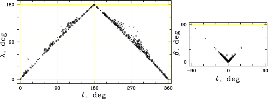
Figure 1: Aspect angles $\lambda$ and $\beta$ versus Galactic coordinates $l$ and $b$, respectively, for all 650 clusters.

Using the equations above, one can compute shape parameters (principal semi-axes $A$ and $B$, ellipticity $e$ and angles $q$, $\beta$), both for real and modelled clusters.

3 Numerical modeling

A non-sphericity of star clusters is predicted both by theory and numerical simulations. Wielen (1974, 1985) predicted that the ratios of the three orthogonal axes of the cluster ellipsoid should show the ratio $(a:b:c)=(2.0:1.4:1.0)$. The largest axis is pointing to the Galactic centre and the smallest one is directed to the North Pole. These results were obtained with N-body calculations of 500 particles, and were confirmed later with somewhat more populated models including up to 1000 particles (Terlevich 1987), and up to 2500 particles (Chumak & Rastorguev 2006). Such a number of particles corresponds to a cluster initial mass below $10^{3}M_{\odot}$. Presently there are evidences, however, that average masses of forming star clusters are larger. For example, Piskunov et al. (2008b) have found, that the average mass of the Galactic open clusters at birth is equal to $4.5\cdot 10^{3}\,m_{\odot}$. Therefore, it is necessary to consider more populated models than it has been done before.

3.1 $\phi$GRAPE N-body code

For our high resolution N-body simulations we use the specially developed $\phi$GRAPE code. The code itself and also the GRAPE hardware we used are described in the paper by Harfst et al. (2007) in more detail. Here we just briefly mention a few of the special features of our code. The program was already thoroughly tested with different N-body applications, including the high resolution, direct study of the dynamical evolution of the Galactic centre with Binary (or Single) Black Holes (Berczik et al. 2005, 2006; Merritt et al. 2007) .

The program acronym $\phi$GRAPE means: Parallel Hermite Integration with GRAPE. The serial and parallel versions of the program are written from scratch in ANSI-C and use the standard MPI library for communication. For the integration of the star cluster’s dynamical evolution inside the Galactic potential we use the parallel GRAPE systems developed at ARI Heidelberg (GRACE - year 2005) and at MAO Kiev (GRAPE/GRID - year 2007).

Table 1: The parameters of the Galactic potential components.

Mass component	$M/m_{\odot}$	$a$, kpc	$b$, kpc
Bulge	$1.4\cdot 10^{10}$	0.0	0.3
Disk	$9.0\cdot 10^{10}$	3.3	0.3
Halo	$7.0\cdot 10^{11}$	0.0	25.0

The code uses the 4-th order Hermite integration scheme for the particles with the hierarchical individual block timesteps, together with the parallel usage of GRAPE6a cards for the hardware calculation of the acceleration $\@vec{a}$ and the first time derivative of the acceleration $\@vec{\dot{a}}$ (this term is usually called “jerk” in the N-body community).

We specially check the effect of N-body softening, which suppresses the hard binary formation in our code, on the evolution of the cluster model. We vary the softening parameter from a few hundreds down to a few astronomical units and do not find a significant difference in the evolution of the cluster mass and shape. We also consider the role of a possible initial mass segregation and do not observe any dependence of the evolution of the semimajor axis on this value.

Compared with the previous public version we add two major changes to the code. First of all we add the possibility to have some external potential, acceleration and also “jerk”. For the external potential we choose the form proposed by Miyamoto & Nagai (1975). Using such a multi-mass component potential we can easily approximate the Galaxy’s external force, acting on our star cluster in the Galactic disk at different Galactocentric distances. The second change includes the possibility to turn on the mass loss due to the stellar evolution for every modelled star particle. For metallicity-dependent stellar lifetimes we use the approximation formula proposed by Raiteri et al. (1996):

$$\log\tau=a_{0}(Z)-a_{1}(Z)\cdot\log m+a_{2}(Z)\cdot\log^{2}m,$$

where $\tau$ is expressed in years, the stellar mass $m$ in solar masses, and where $Z$ is the abundance of heavy elements. The coefficients are defined as:

$$\begin{array}[]{lllll}a_{0}(Z)=10.130+0.0755\cdot\log Z-0.0081\cdot\log^{2}Z,\\ a_{1}(Z)=4.4240+0.7939\cdot\log Z+0.1187\cdot\log^{2}Z,\\ a_{2}(Z)=1.2620+0.3385\cdot\log Z+0.0542\cdot\log^{2}Z.\\ \end{array}$$

The mass lost by stars during their evolution is calculated with the help of tables from the paper of van den Hoek & Groenewegen (1997) and is approximated analytically via the metallicity-dependent formula:

$$m_{eject}=-0.4205\cdot Z^{-0.0177}+(0.9015+0.6294\cdot Z)\cdot m_{init}.$$

For simplicity, we assume in our model that stars loose their masses permanently with a constant rate: $-m_{eject}/\tau$.

Since stars lose the bulk of their masses at the end of their evolution, we test, also, an alternative mass loss scenario, where we reduce the stellar masses just in one timestep at the end of the star life. We find that the models show almost the same evolutionary patterns for shape parameters and mass loss of clusters independent of the version of stellar mass loss used.

3.2 Initial conditions for the star cluster

Table 2: The list of model parameters: initial mass $M_{c}(0)$, number of particles $N$, cluster radius $R_{c}$, distance from the Galactic center $R_{0}$, circular velocity $V_{0}$, time step $\delta t$, dimensionless angular velocity $\omega_{0}$; concentration parameter $W_{0}=6.0$.

$M_{c}(0),$	$N$	$R_{c}$,	$R_{0}$,	$V_{0}$,	$\delta t$,	$\omega_{0}$
$m_{\odot}$		pc	kpc	km/s	Myr
$10^{3}$	4040	3	7.0	236	2.45	0.0, 0.3, 0.6
$10^{3}$	4040	3	8.5	233	2.45	0.0, 0.3, 0.6
$10^{3}$	4040	3	10.0	231	2.45	0.0, 0.3, 0.6
$5\cdot 10^{3}$	20202	7	7.0	236	3.91	0.0, 0.3, 0.6
$5\cdot 10^{3}$	20202	7	8.5	233	3.91	0.0, 0.3, 0.6
$5\cdot 10^{3}$	20202	7	10.0	231	3.91	0.0, 0.3, 0.6
$10^{4}$	40404	10	7.0	236	4.71	0.0, 0.3, 0.6
$10^{4}$	40404	10	8.5	233	4.71	0.0, 0.3, 0.6
$10^{4}$	40404	10	10.0	231	4.71	0.0, 0.3, 0.6

For the generation of the initial position and velocity distributions of cluster particles we use the standard King model. The code for the generation of the initial rotating star cluster is described in detail by Einsel & Spurzem (1999). We also use their notation to parametrize our rotating King model family with the concentration parameter $W_{0}$ and the dimensionless angular velocity $\omega_{0}$. Thus each model can be parametrized by the combination of these two numbers. The larger $W_{0}$ the larger is the central concentration. The larger $\omega_{0}$ the larger is the angular momentum of the model.

For the present simulations we use the variation with three basic King models only. We vary only the rotation parameter $\omega_{0}=(0.0,\leavevmode\nobreak\ 0.3,\leavevmode\nobreak\ 0.6)$. According to Table 1 in Einsel & Spurzem (1999) the ratio of the “pure” rotational energy to the total kinetic energy of the model for these three cases is $E_{rot}/E_{kin}=(0.0,\leavevmode\nobreak\ 0.105,\leavevmode\nobreak\ 0.278)$. The concentration parameter was always set to $W_{0}=6.0$ (which corresponds to the models with medium concentration).

As a next step, taking the Salpeter (1955) initial mass function (IMF) $f(m)=dN/dm$, we create the random particle mass distribution:

$$dn(m)=f(m)\cdot dm={\it C}\cdot m^{-(1+\alpha)}\cdot dm,$$

with the lower and upper mass limits $m_{l}=0.08\leavevmode\nobreak\ m_{\odot}$, $m_{u}=8.0\leavevmode\nobreak\ m_{\odot}$ and with Salpeter’s slope $\alpha=1.35$. We use the upper mass limit of 8.0 $m_{\odot}$, because we consider a “pure/classical” open cluster (older than 30…40 Myr), when all high mass stars have already finished their life as a SNII, and swept out all the residual gas left from the cluster formation process.

The necessary number of particles for a given initial mass of the cluster $M_{c}(0)$, can be computed from the assumed IMF as

$$N=M_{c}(0)\cdot\frac{-\alpha+1}{-\alpha}\cdot\frac{(m_{u}^{-\alpha}-m_{l}^{-\alpha})}{(m_{u}^{-\alpha+1}-m_{l}^{-\alpha+1})}.$$

With the adopted IMF parameters for the model cluster and initial masses $M_{c}(0)=(10^{4},5\cdot 10^{3},10^{3})\leavevmode\nobreak\ m_{\odot}$ we have the following particle numbers $N$ = (40404, 20202, 4040).

After our setting of initial masses, positions and velocities of every particle in the model, we do the standard N-body normalization (Aarseth et al. 1974) of the model, and rescale the initial cluster data to put our system into virial equilibrium $E_{gra}=-2\cdot E_{kin}=2\cdot E_{tot}$ with the following parameters: $G=M_{c}=1$ and $E_{tot}=-0.25$. This step does not change any physical quantities of the modelled star cluster, but is just very useful for numerical reasons. For a King model with $W_{0}=6.0$ such a normalization produces a half-mass radius of about 0.8 (in dimensionless units).

After the construction of dimensionless parameters of our model we can easily extend them to a different physical cluster mass and half-mass radius. In principle, these two parameters can be set independently, but in order to reduce the number of independent initial parameters we decide to use some physically motivated relation between initial mass and initial half-mass radius. For this purpose we use the extension of the well known mass vs. radius relation for molecular clouds and clumps in the Galaxy (see Theis & Hensler 1993; Inoue & Kamaya 2000), which can be scaled as:

$$R_{c}\approx 100\cdot\sqrt{\frac{M_{c}}{10^{6}\leavevmode\nobreak\ m_{\odot}}}\leavevmode\nobreak\ \leavevmode\nobreak\ {\rm pc}$$

For the three physical masses chosen we set the corresponding radii to $R_{c}$ = (10, 7, 3) pc.

In order to check the dependence of the computed evolution of cluster shape on the adopted mass vs. radius relation, we run a series of models where we set the normalising factor to 100, 71, and 43 pc. We find that for typical model parameters, the evolution of the cluster shape does not depend on this factor, in practice.

3.3 Galactic rotation curve

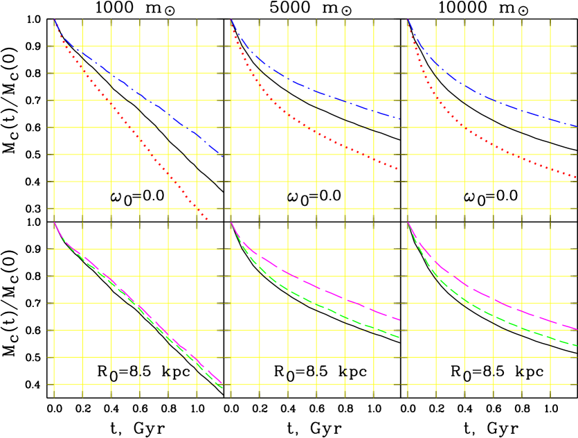
Figure 2: The evolution of the mass of dynamically bound particles for three cases of the initial mass of the cluster models (three columns with masses shown at the top of each column). The upper panels are constructed for non-rotating models ($\omega_{0}$ = 0.0) and show the effect of the Galactocentric distance. The dotted (red), solid (black) and dashed-dotted (blue) curves are models at $R_{0}=$ 7, 8.5 and 10 kpc. The bottom panels illustrate the effect of cluster rotation at the Solar Galactocentric distance. The solid (black), dashed (green) and long dashed (magenta) curves show models with $\omega_{0}=$ 0.0, 0.3 and 0.6.

For the external Galactic potential shaping a cluster we choose the combined “Plummer-Kuzmin disk” form (see Miyamoto & Nagai 1975):

$$\Phi(r,z)=-\frac{G\cdot M}{\sqrt{r^{2}+(a+\sqrt{b^{2}+z^{2}})^{2}}}.$$

Coupling such a potential with a three-component Galactic mass distribution model comprised of “Bulge”, “Disk”, “Halo” components (Douphole & Colin 1995) one can easily reproduce the observed rotation curve of the Galaxy

$$\frac{V^{2}(r)}{r}=-\nabla\Phi_{Bulge}(r,z)-\nabla\Phi_{Disk}(r,z)-\nabla\Phi_{Halo}(r,z).$$

In order to bring this into agreement with the kinematics of the open cluster subsystem in the Solar neighborhood we slightly modify the Douphole & Colin (1995) parameters. The parameter values consistent with the observed Oort constants $(A,B)=(14.5\pm 0.8,-13.0\pm 1.1)$ km/s/kpc derived by Piskunov et al. (2006) are shown in Table. 1. The adopted values of Oort constants correspond to $V/R_{\odot}=27.5\pm 1.3$ km/s/kpc, which at $R_{\odot}$ = 8.5 kpc gives $V\approx$ 233 km/s. Using these data we derive circular velocities at distances of 7.5 kpc and 10.0 kpc from the Galactic centre, too.

3.4 Model list and model cluster memberships

As a starting point for our model cluster, we select the position inside the Galactic disk ($R_{0}$, 0.0, 0.0) with the corresponding circular velocity (0.0, $-V_{0}$, 0.0). For the set of our runs we use three values for the positions inside the Galactic disk: $R_{0}$ = (7.0, 8.5, 10.0) kpc with corresponding circular velocities $V_{0}$ = (236, 233, 231) km/s. Together with the three initial masses $M_{c}(0)$ of clusters and with the three rotational parameters $\omega_{0}$ these three positions create the set of 3 $\times$ 3 $\times$ 3, i.e. in total 27 models (see the full list of model parameters in Table 2). Each model comprises a few hundreds of “snapshots” made at different moments of time equally spaced from $t=0$ to $t\gtrsim 1$ Gyr. For each model particle, every snapshot displays its initial and current mass, coordinates and velocities in the rectangular Galactocentric coordinate system.

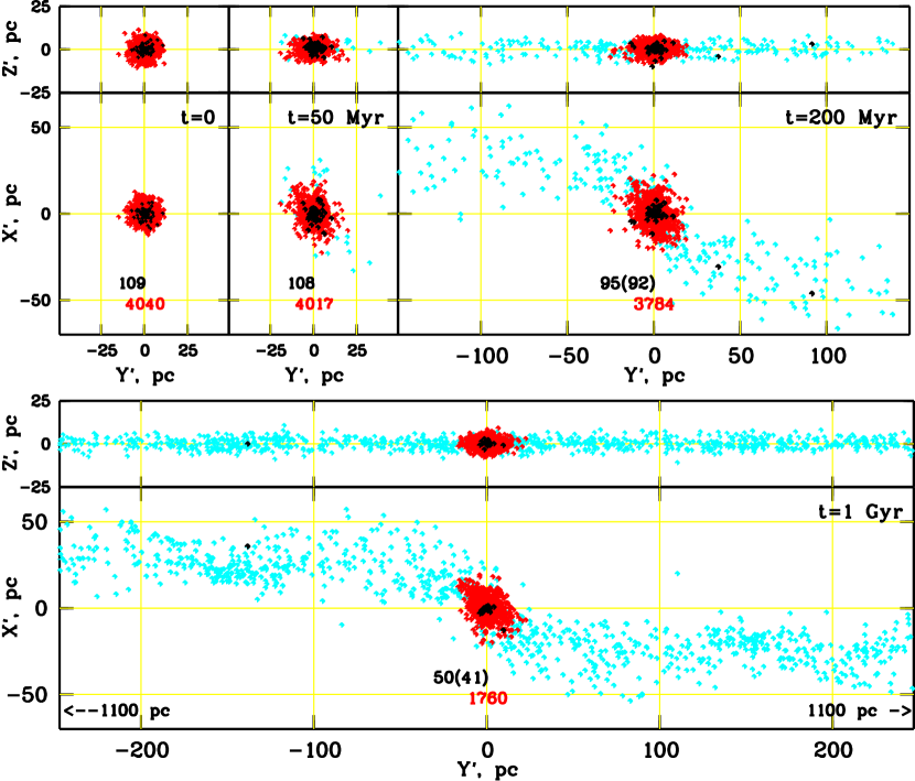
Figure 3: The particle distribution in the $X^{\prime}Y^{\prime}-$ and $Z^{\prime}Y^{\prime}-$ planes of a model with initial mass $M_{c}(0)=10^{3}m_{\odot}$ and distance from the Galactic centre $R_{0}$ = 8.5 kpc at different moments of time. The cluster age is indicated in the right corner of each panel. Cyan dots - all particles, red dots and red-color labels - dynamically bound particles, black dots and labels - massive particles ($m>1m_{\odot}$), black labels in brackets - dynamically bound massive particles. Arrows indicate the limits of cluster tails when they do not fit to the frame.

To provide the detailed analysis of star cluster shapes we need to find the cluster centre position, at first. This issue requires special attention, since particles having left the cluster during the evolution should not be taken into account for this purpose. For this we use our own iterative routine considering the distributions of positions and velocities of particles and apply it to every snapshot. We find that we are able to determine the centre even for models with highest mass loss, which lose more than half of their initial content during the evolution.

As a next step in our analysis, we convert the positions and velocities of the particles into the proper coordinate system of the cluster related to the local density centre and define the list of particles which are still bound to the cluster. We use the particle kinetic and gravitational energy as criteria of belonging to the cluster. The kinetic energy is computed from the velocity of every particle in the proper system of the cluster. For the gravitational energy we use the value of the cluster’s self-gravity potential, determined as the sum of all interactions between a selected particle and the rest of the particles. We assume, that only the particles which have a negative relative energy are still bound to the cluster:

$$|E^{gra}_{i}|>E^{kin}_{i}.$$

In other words, for bound particles we can write:

$$|\varphi_{i}|>\frac{|\mathbf{v}_{i}|}{2}.$$ (3)

Using such a condition for the definition of cluster membership, we exclude particles which have relatively large velocities compared to the cluster centre and construct a list of particles which we select to be “dynamical” cluster members.

We define the current mass of the cluster $M_{c}(t)$ as the sum of masses of all bound particles. In Fig. 2 we show the evolution of $M_{c}(t)$ for a set of selected models. The evolution shows a similar behaviour as in the models of Ernst et al. (2007) and Kim et al. (2008). Fig. 2 indicates, that a star cluster looses from 35% to 70% of its initial mass during the first 1 Gyr and the mass loss is decreasing with increasing distance of clusters from the Galactic centre and with increasing cluster rotation velocity.

We double check our mass loss sequences by comparing with the results which we obtain with other fully independent and also publicly available N-body codes (N-body4 (with GRAPE6) & N-body6++). All the models show the very same evolution patterns of mass loss.

4 Shape parameters of observed and modelled clusters

4.1 Shape parameters of the cluster models

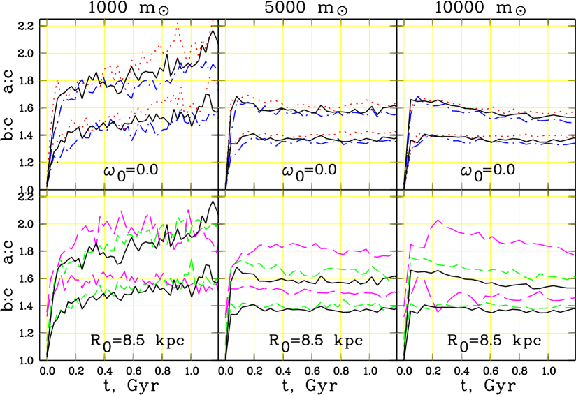
Figure 4: The evolution of ratios of the model ellipsoidal axes $a:c$ and $b:c$ for bound particles for models of different initial mass (three columns with masses shown at the panel top). In every panel the upper triplet of the curves indicates the $a:c$ ratio and the lower triplet corresponds to $b:c$. The designations are the same as in Fig. 2.

Let us first consider how the cluster model, initialized as a spheroid, changes its shape and orientation with time. The evolution of a selected model in the planes $X^{\prime}Y^{\prime}$ and $Y^{\prime}Z^{\prime}$ is shown in Fig. 3. With time the cluster elongates along the line of the Galactocentric radius, and begins to “leak” losing low-mass particles from the limits corresponding to the Lagrangian points, farthest and nearest to the Galactic centre. Because of the differential rotation the particles overtake the cluster at the end nearest to the Galactic centre and lag it at the farthest end. The tails contain stars, which are not bound to the cluster anymore. The dynamical members form an ellipsoid projected onto the $X^{\prime}Y^{\prime}$ and $Z^{\prime}Y^{\prime}$ planes as ellipses. In the $X^{\prime}Y^{\prime}$ plane the ellipse is tilted with respect to the $X^{\prime}$-axis at an angle $q_{XY}$, whereas in the $Z^{\prime}Y^{\prime}$- plane it follows the $Y^{\prime}$-axis.

Such details in the distribution of N-body particles arise due to interaction with the Galactic tidal field. They are found in all N-body simulations of open clusters (see, e.g. Fig.7 of Terlevich 1987; Chumak & Rastorguev 2006).

In Fig. 3 one can also clearly see the so-called “tidal tail clumps” (star density enhancements) at about 150 pc from the cluster centre. Such clumps were mentioned probably for the first time in Capuzzo Dolcetta et al. (2005) and were discussed in more detail recently by Küpper et al. (2008). We observe such clumps in all our models (see the model videos at the FTP link shown in the footnote on page 2). They can be explained by a simple theory (Just et al. 2008).

In Fig. 4 and Fig. 5 we show the evolution of the axis ratios $a:c$ and $b:c$ and of the tilt angle $q_{XY}$ for selected models. Already after a few tens of Myrs the initially spherical cluster transforms into an ellipsoid tilted with respect to the Galactocentric radius, with the semi-major axis about twice as large as the minor one, and a tilt between $30^{\circ}$ and $40^{\circ}$. The shape parameters are almost independent of the Galactocentric distance of the model clusters, but the ellipsoid becomes flatter with increasing cluster rotation.

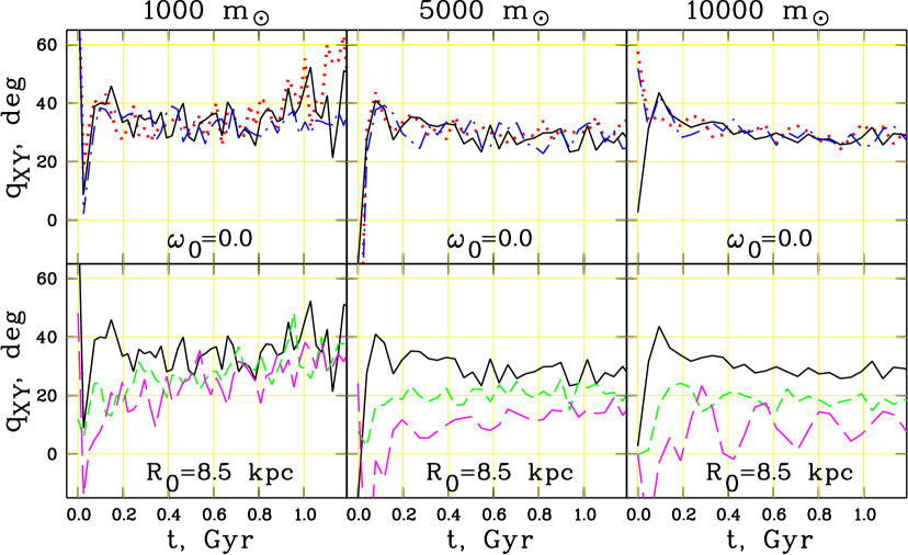
Figure 5: The evolution of the tilt angle $q_{XY}$ computed for dynamically bound particles for three cases of the initial mass of the cluster models (three columns with masses shown in the top of the panels). The designations are the same as in Fig. 2.

N-body models offer good possibilities for studying various biases which can occur in cluster ellipticities derived from observations. In Fig. 6 we show the dependence of the ellipticity of a model cluster on sampling constraints due to the mass and the distances from the cluster centre of the particles considered. In this way we mimic the usual selection effects which impact the observations of real clusters. Cutting the model particles at a certain mass limit simulates a possible bias due to a limited deepness of a survey. The restriction of the models by distances of particles from the cluster centre simulates the bias arising due to underestimation of cluster size. Hereafter, we call the latter effect a “restricted area bias”. We consider a cluster model, where both major and minor semi-axes of the ellipsoid are seen under a right angle, i.e. the projected ellipticity is at its maximum. The model cluster is 150 Myr old, its current mass is $4.2\cdot 10^{3}\,m_{\odot}$, and, as a consequence, its tidal radius is $r_{t}=22.5$. The number of dynamically bound particles is $N_{c}=19371$.

The tidal radius of the model cluster was computed from the current total mass of member particles with the well known relation from King (1962). This places the model tidal radii into the same system as the observed tidal radii of open clusters. Note that for about 1/3 of our clusters, we determined tidal radii by a fit of the cluster radial density distribution to a King profile (Piskunov et al. 2007), and for the remaining clusters we used a proper calibration to estimate their tidal radii (Piskunov et al. 2008a). Then, assuming that clusters fill up their potential well, the cluster “tidal” masses were computed from the King (1962) formula for all 650 clusters.

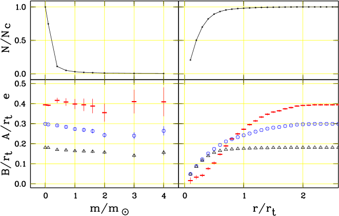
Figure 6: Dependence of the shape of a model cluster on the sampling constraints. Bottom: cluster ellipticity $e$ and semiaxes $A$ and $B$ as functions of lower mass limit (left) and radius of the considered area (right). The circles show the major semiaxes, the triangles are for the minor one, and short (red) horizontal bars mark the ellipticity. Vertical bars indicate the statistical uncertainties. The upper row shows the numbers of particles participating in the construction of the corresponding values.

From Fig. 6 we conclude that excluding low-mass particles from the consideration has a much smaller impact onto the resulting ellipticity, than excluding the external parts of the model cluster from consideration. Indeed, a removing of low-mass particles causes the axes $A$ and $B$ to slightly decrease. Since they change, however, in coordination to each other, the ellipticity is about constant within the statistical uncertainties. In contrast, with including more and more distant particles in the ellipticity calculation, the ellipticity increases steadily. At a distance of two tidal radii, the corresponding ellipticity is close to the limiting value which is achieved if all bound particles within about three tidal radii are taken into account.

This behaviour can be easily understood if one considers radial dependences of the axes $A$ and $B$. The minor axis $B$ reaches its maximum value already within $r_{t}$ and does not increase anymore, whereas the major axis $A$ continues to rise beyond the tidal radius. One should note that the cluster flatness is produced by a relatively small number of cluster particles: only 2% of bound particles occupy a zone beyond $1\,r_{t}$, and only 0.1% of them can be found at $r>2\,r_{t}$. In contrast, a few tens of the most massive particles, which are not constrained spatially, produce about the same ellipticity, as the rest of low mass members. A consequence of a smaller sample is, however, a considerably higher statistical uncertainty in the resulting ellipticity. A comparison with older models shows that the above conclusions are still valid for cluster ages up to one Gyr.

In summary we conclude that the determination of cluster ellipticity is not influenced strongly by the survey’s deepness, but rather by the sizes of the surveyed areas around the clusters. Restricting to areas smaller than the corresponding tidal radius one takes a risk to introduce a “restricted area bias” in the resulting cluster ellipticities, hence making clusters more circular than they are in reality.

4.2 Determination of the uniform shape parameters of the observed and modelled clusters

In order to compare the observations with models, one needs parameters adequately describing both entities. From observations, we compute apparent ellipticities $e$ and orientation parameters $q$ for each cluster of our sample using the approach presented in Sec. 2 and adopting the apparent cluster radius $r_{2}$ from Kharchenko et al. (2005a, b). The observed shape parameters $e$ and $q$ for each of the 650 open clusters are listed in a table that is available in electronic form only. It can be retrieved from the CDS. To compute the parameters, we consider only the most probable members, with kinematic and photometric probabilities higher than 61% (see Kharchenko et al. 2004). This decision was simply guided by the fact that a sample was stronger contaminated if we included stars with lower membership probability. Since field stars tend to a random distribution, the contamination leads to a bias: a fictitious decrease of the observed ellipticity.

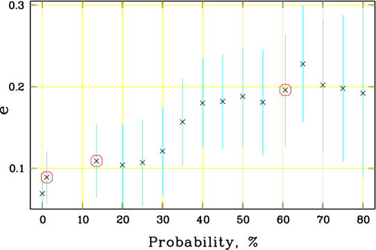
Figure 7: Dependence of the apparent ellipticity $e$ on the probability threshold for cluster membership for the open cluster Stock 2. The bars correspond to mean errors. Large open circles indicate the apparent ellipticities based on the sample of stars with membership probability larger than 1%(the left circle), larger than 14%(the middle circle), larger than 61%(the right circle).

For illustration, we carried out the ellipticity calculation considering cluster stars of different membership probability. For our basic sample of 152 clusters (see Sec. 4.3 for definition), we obtain an average ellipticity of $\overline{e}=0.18$ when we consider stars with a membership probability better than 61%, $\overline{e}=0.14$ with membership probability better than 14%, $\overline{e}=0.12$ with membership probability better than 1%, and $\overline{e}=0.09$ if we consider all stars projected on the cluster area. A probability threshold of 61% is a compromise between a possible bias due to backgroud contamination and the number of stars included in the ellipticity calculation.

On the other hand, one must make certain that stars with membership probability larger than 61% describe adequately the cluster properties. In Fig. 7 we show the variations of the apparent ellipticity with the probability threshold in the case of the cluster Stock 2, for example. This cluster is a well populated cluster, so we get satisfactory statistics even for the smallest star samples containing the most probable cluster members. The contamination effect by field stars is strong if the probability threshold $P$ is less than 30%, but it becomes almost insignificant (although still systematic) at $40\%\leqslant P<60\%$. If we consider stars with membership probabilities larger than 60%, the variations in the resulting apparent ellipticity have a random character. This indicates that - although the sample of stars with membership probability over the 61% threshold may contain a number of field stars - they do not introduce a bias in the apparent ellipticity determination. A further increase of the probability threshold does not improve the results significantly, but the mean error of the apparent ellipticities becomes larger due to poor statistics. Therefore, we consider the choice of a 61% threshold to be the optimum.

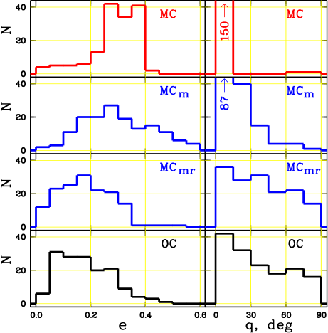
Figure 8: Distributions of ellipticities $e$ (left panels) and orientation angles $q$ (right panels) for 152 clusters. The panels are marked with the identifiers of the set.

From the models, we obtain the axes $a$, $b$, $c$ and the tilt angle $q_{XY}$ describing the shape and orientation of a cluster in the proper coordinate system ($X^{\prime},Y^{\prime},Z^{\prime}$). To compare them with the observed parameters $e$ and $q$, we must “view” the models under the same conditions which are valid for the observed clusters. First, one has to remember that the limiting magnitude of the ASCC-2.5 is about $V=12$, and even in the nearest clusters we can, therefore, observe only stars more massive than $0.7\,M_{\odot}$, i.e. one order of magnitude higher than the lower mass limit of model particles. Further, the resulting shape parameters are strongly dependent on the size of the area around the cluster centre included in the computations. Therefore, a model cluster must be scaled to the apparent cluster radius $r_{2}$ of its observed counterpart.

For each observed cluster, we first selected its theoretical counterpart from Table 2 at the Galactocentric distance which best fits the location of the observed cluster. Then, for a given model we selected a snapshot with an age closest to the observed age. This snapshot was placed at the position of the real cluster, and the model particles were projected onto the face-on plane (i.e. for every particle the standard coordinates $x,y$ were computed). From the complete list of model particles, we selected the actual members of the cluster by applying eq. (3). We used this list to compute “true” model parameters of the cluster’s shape with the formulae from Sec. 2.

The models contain particles down to relatively low masses which can not always be detected in real observations. In order to reproduce the observed conditions (i.e. to obtain “observed” model parameters), we further diminished the list of dynamical members selecting particles in the observed mass range and obeying the condition that the number of modelled and observed members within the cluster area $r_{2}$ is approximately the same.

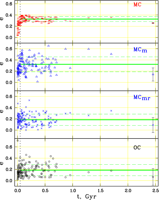
Figure 9: Ellipticities $e$ of 144 low-latitude open clusters ($\beta<20^{\circ}$) versus age $t$. The panels are marked with the identifiers of the set. The dotted vertical line marks $t=50$ Myr. In each panel, the horizontal lines show the corresponding average ellipticity for clusters older than 50 Myr. The dashed lines indicate their standard deviations. Vertical bars for a cluster at $t=2.46$ Gyr show typical $rms$ errors of the ellipticity estimates.

Table 3: Projected semi-axes $A$ and $B$ in selected directions of the sky for the model of preferentially oriented cluster ellipsoids.

Case	$\lambda$	$\beta$	semi-major axis $A$	semi-minor axis $B$
1)	$0^{\circ}\dots 180^{\circ}$	$0^{\circ}$	$a\cdot b/\sqrt{a^{2}\cdot\cos^{2}(\lambda-q_{XY})+b^{2}\cdot\sin^{2}(\lambda-q_{XY})}$	$c$
2)	$\lambda_{ac}$	$0^{\circ}\dots 90^{\circ}$	$a$	$c\cdot b/\sqrt{b^{2}\cdot\cos^{2}\beta+c^{2}\cdot\sin^{2}\beta}$
3a)	$\lambda_{bc}$	$0^{\circ}\dots\beta_{0}$	$b$	$c\cdot a/\sqrt{a^{2}\cdot\cos^{2}\beta+c^{2}\cdot\sin^{2}\beta}$
3b)	$\lambda_{bc}$	$\beta_{0}\dots 90^{\circ}$	$c\cdot a/\sqrt{a^{2}\cdot\cos^{2}\beta+c^{2}\cdot\sin^{2}\beta}$	$b$

As a result, we consider four different sets of input data. The first set includes real observations of clusters. We call this set “OC”. The following three sets are related to the models. The set “MC” represents the models as such, and reproduces “true” clusters containing all the dynamical members in the complete range of particle masses. The third set “$\mathrm{MC_{m}}$” includes only “massive” dynamical members of given clusters which are above the limiting magnitude of ASCC-2.5. Finally, the set “$\mathrm{MC_{mr}}$” completely reproduces the observed sample: it includes the same number of particles selected in the same mass range $\Delta m$ as we do observe in real clusters. Similar to the observed clusters, the $\mathrm{MC_{mr}}$ models contain only those particles, which reside within the apparent cluster radius $r_{2}$. Since the sets $\mathrm{MC_{m}}$ and $\mathrm{MC_{mr}}$ bridge the sets MC and OC, they are introduced to investigate the biases in the observed shape parameters which may occur due to the limitations of mass ranges and spatial distribution of cluster stars described in Sec. 4.1.

4.3 Comparison of shape parameters of the modelled and observed clusters

For comparison with the model data we consider only clusters with more than 20 most probable members. We also exclude the two very populated clusters NGC 869 ($h$ Per) and NGC 884 ($\chi$ Per), as they are overlapping in the projection onto the sky, and have a large number (more than 50%) of members in common, making an accurate determination of their individual shape parameters rather difficult. Hereafter, we refer to the resulting sample as the “basic sample” comprising 152 objects.

According to the mass estimates of open clusters given in Piskunov et al. (2008a), the average tidal mass of clusters in the basic sample turns out to be about $10^{3}m_{\odot}$ which is comparable to the average cluster mass of $700\,m_{\odot}$ determined in Piskunov et al. (2008b) for the complete cluster sample of 650 clusters. Therefore, we assume that the basic sample represents sufficiently well the typical cluster population in the Solar vicinity, having typical initial masses about $4.5\cdot 10^{3}\,m_{\odot}$ as determined in Piskunov et al. (2008b). For this reason, we select the cluster models with initial mass of $5\cdot 10^{3}m_{\odot}$ as the most suitable ones for comparison with observations. According to Fig. 4, the shape parameters do not change considerably for models with larger initial masses, whereas the ellipticity becomes more prominent in clusters with initial masses considerably lower than the adopted $5\cdot 10^{3}m_{\odot}$. In the following we consider the non-rotating models of open clusters keeping in mind that with increasing rotation velocity clusters become also flatter.

The distributions of ellipticities $e$ and orientation angles $q$ of the observed and modelled clusters of the basic sample are shown in Fig. 8. The distribution of ellipticity shows a clear maximum for the complete cluster models (the set MC) at $e\approx 0.25\dots 0.35$, and the corresponding ellipsoids are elongated parallel to the Galactic plane (the orientation angle $q\approx 0^{\circ}$). For the models $\mathrm{MC_{m}}$ and $\mathrm{MC_{mr}}$ which take into account the restrictions set by observations, the ellipticity decreases, while the spread in $q$ increases indicating a more random orientation of the apparent ellipses. The observed clusters (the set OC) show relatively small ellipticities with a peak between $0.075\dots 0.175$. Although a peak at $q=0$ is still observed, the orientation angles $q$ are distributed over the whole range. This is simply a consequence of small ellipticities since apparently circular clusters have no orientation angle.

We show the dependence of ellipticities $e$ on cluster age for all the four sets in Fig. 9. We limit our consideration to 144 clusters with $\beta<20^{\circ}$ in order to minimize the impact of the projection onto the smallest axis of the ellipsoid occurring for clusters at large galactic latitudes. According to the model set MC, clusters change their initially circular shapes into ellipsoids during the first 50 Myr and keep this form thereafter. This behaviour can be also concluded from Fig. 3. The small scatter around the average ellipticity for clusters older than 50 Myr is defined by their location in the Galactic plane relative to the Sun and to the Galactic centre, i.e. by the aspect angle $\lambda$. When we reduce the number of observable members by excluding model particles of low masses (the set $\mathrm{MC_{m}}$), the average ellipticity does not change, although the distribution shows a larger scatter which arises due to poorer statistics of the remaining dynamical members. When further excluding model particles located outside the apparent radius assumed for the clusters, the average ellipticity becomes significantly smaller. The observed clusters show a similar ellipticity distribution as the model set $\mathrm{MC_{mr}}$. These features confirm the analysis carried out in Sec. 4.1.

The following statistics supports the decisive role of spatial limitation ($r\leq r_{2}$) hiding the real ellipticity of clusters. The average ellipticities of 103 clusters with $t>50$ Myr are equal to $0.328\pm 0.004$, $0.322\pm 0.013$, $0.184\pm 0.010$, $0.186\pm 0.010$ for MC, $\mathrm{MC_{m}}$, $\mathrm{MC_{mr}}$ and CO, respectively. The similar average ellipticities of the sets $\mathrm{MC_{mr}}$ and OC indicate that a possible bias due to background contamination is rather small if the ellipticity calculation is based on cluster stars with membership probabilities higher than 61%. We conclude, also, that a spatial limitation of cluster members introduces a significant bias in the determination of ellipticities, whereas a mass limitation increases mainly the random uncertainties of the results. The smaller ellipticities of the sets $\mathrm{MC_{mr}}$ and OC are results of too small radii $r_{2}$ assumed for the clusters. Note that, on average, the ASCC-2.5-based estimates of cluster radii $r_{2}$ (Kharchenko et al. 2005a) are already larger by a factor of two compared to previously published values. Better estimates of cluster radii are only possible if a proper separation of cluster members from the numerous field stars can be achieved in outer cluster regions. This would require more accurate surveys of proper motions and photometric data all over the sky. On the other hand, surveys deeper than the ASCC-2.5 would increase the random accuracy of the ellipticity determination of open clusters.

4.4 Distribution of the cluster ellipticity over the sky

Up to now, the ellipticity of open clusters was studied either for individual objects (Raboud & Mermilliod 1998a, b), or in selected directions of the Galactic disk (Chen et al. 2004). In the present study we determined the apparent shape parameters for clusters observed all over the sky. Therefore, it seems to be useful to derive geometric relations between the apparent ellipticity of clusters and their spatial location in the Galaxy. Of course, a regular dependence can only be expected if cluster ellipsoids are not orientated randomly in space but show a certain orientation with respect to the Galactic centre.

Indeed, the model calculations indicate that the Galactic tidal field and differential rotation quickly align clusters along a preferential direction, and the resulting ellipsoids show always the same axes ratios. Let $a,\,b,\,c$ be the semi-axes of these three-axial ellipsoids with the semi-major axis $a$ tilted with respect to the Galactocentric radii of the clusters by an angle $q_{XY}$. For simplicity, we further assume that the major axis is parallel to the Galactic plane. Hereafter, we call this approach the model of preferentially-oriented ellipsoids, and the ellipsoid itself the “reference” one.

From observations, however, we can only see a two-dimensional projection of the reference ellipsoid on the sky that is an ellipse with the semi-axes $A$ and $B$. The ratio $B/A$ varies from $c/a$ to 1, depending on the aspect angles $\lambda$ and $\beta$ describing the cluster location with respect to the Sun and the Galactic centre. The apparent ellipticity $e$ changes from 0 to $1-c/a$, respectively.

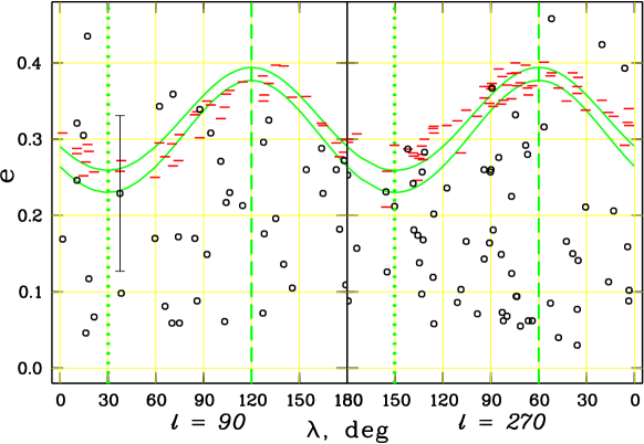
Figure 10: Ellipticity $e$ versus aspect angle $\lambda$ for 103 clusters with $\beta<20^{\circ}$ and $t>50$ Myr. The left panel corresponds to the Galactic longitude range $l=0^{\circ}...180^{\circ}$, the right panel to $l=180^{\circ}...360^{\circ}$. The curves show the $e(\lambda,\beta)$–relations for $\beta=0^{\circ}$ (upper curve) and $\beta=20^{\circ}$ (lower curve) constructed for the reference ellipsoid tilted to the direction to the Galactic centre by angle $q_{XY}=30^{\circ}$, having axes ratios (1.65 : 1.35 : 1). Short horizontal bars (red): set MC (complete models), open circles: set OC (observations). The vertical bars drawn for one object show the typical $rms$ error of the observed ellipticity. The dashed vertical lines mark $\lambda_{ac}$, the dotted ones $\lambda_{bc}$.

When a cluster is located in the Galactic plane ($b=\beta=0^{\circ}$), $B=c$ is always valid, and $A$ varies from $b$ to $a$. The apparent ellipticity reaches the maximum $e=1-c/a$ at aspect angles $\lambda_{ac}=90^{\circ}+q_{XY}$ (for $l=0^{\circ}\dots 180^{\circ}$) and at $\lambda_{ac}=90^{\circ}-q_{XY}$ (for $l=180^{\circ}\dots 360^{\circ}$). In contrary, the apparent ellipticity reaches the minimum $e=1-c/b$ at $\lambda_{bc}=q_{XY}$ (for $l=0^{\circ}\dots 180^{\circ}$) and $\lambda_{bc}=180^{\circ}-q_{XY}$ (for $l=180^{\circ}\dots 360^{\circ}$). For all other directions, the apparent ellipticities can be computed from the equations given in the first row of Table 3.

Though the majority of star clusters is located near the Galactic plane, there is a number of clusters at higher galactic latitudes. In a special case, when clusters are located directly at the Galactic Poles, one observes $A=a$ and $B=b$. For all other clusters outside the Galactic plane, the projection of the reference ellipsoid is defined by both aspect angles. For example, at $\lambda=\lambda_{ac}$ the ellipticity decreases monotonically from $1-c/a$ at $\beta=0^{\circ}$ to $1-b/a$ at $\beta=90^{\circ}$. The corresponding expression is given in the second row of Table 3. At $\lambda=\lambda_{bc}$ this relation is rather different since the projected ellipse changes its orientation at some angle $\beta_{0}$. Thus the ellipticity first decreases from $1-c/b$ at $\beta=0^{\circ}$ to 0 at $\beta=\beta_{0}$, and then increases to $1-b/a$ at $\beta=90^{\circ}$. The corresponding equations are listed in the last two rows of Table 3. The aspect angle $\beta_{0}$ where the projection becomes a circle ($A=B$) is determined by the semi-axes $a$, $b$, $c$ of the reference ellipsoid from the equality condition

$$b=\frac{c\cdot a}{\sqrt{a^{2}\cdot\cos^{2}\beta_{0}+c^{2}\cdot\sin^{2}\beta_{0}}}.$$ (4)

For given parameters of the reference ellipsoid, the Galactic meridian at $\lambda_{ac}$ defines a locus of maximum ellipticities $e(\lambda_{ac},\beta)$ over the sky, whereas the Galactic meridian at $\lambda_{bc}$ gives a locus of minimum ellipticities $e(\lambda_{bc},\beta)$.

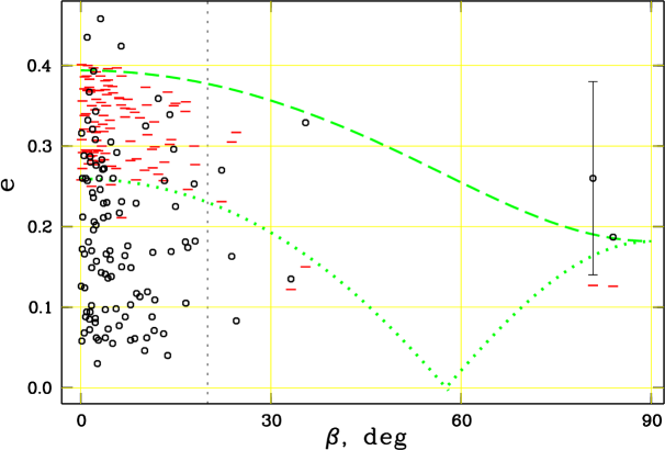
Figure 11: Ellipticity $e$ versus aspect angle $\beta$ for 110 clusters with $t>50$ Myr. The curves show the $e(\lambda,\beta)$–relations for $\lambda=\lambda_{ac}$ (dashed curve) and $\lambda=\lambda_{bc}$ (dotted curve) constructed for the reference ellipsoid tilted to the direction of the Galactic centre by an angle $q_{XY}=30^{\circ}$, and with axes ratios (1.65 : 1.35 : 1). Short horizontal bars (red): MC (complete models), open circles: OC (observations). The vertical bars drawn for one object show the typical $rms$ error of the observed ellipticity. The dashed vertical line marks $\beta=20^{\circ}$.

In Fig. 10 and Fig. 11 we plot the analytical relations from Table 3 together with the model and observed data on ellipticities versus the aspect angles for “relaxed” clusters which are older than 50 Myr. Though a few observed ellipticities fit the predicted values, the majority of the observed clusters show, as expected, too low ellipticities due to the restricted area bias described above. Therefore, we cannot use the observations for deriving the parameters of the reference ellipsoid. Instead, the parameters $a,\,b,\,c$ and $q_{XY}$ were found by fitting the relations from Table 3 to the data points of the complete models (MC) as $(a:b:c)=(1.65:1.35:1)$ and $q_{XY}=30^{\circ}$. These parameters are based on the non-rotating models assuming the same initial masses ($5\cdot 10^{3}M_{\odot}$) but different location of clusters from the Galactic centre (see also Fig. 4 and Fig. 5). For this reference ellipsoid, the angle $\beta_{0}$ is determined from eq. (4) to be $\beta_{0}=57.6^{\circ}$.

4.5 Comparison with the literature

In the literature, there are only a few studies on the ellipticity of Galactic open clusters. Raboud & Mermilliod (1998a) and Raboud & Mermilliod (1998b) studied the shape of the Pleiades and Praesepe using the best data on astrometric and photometric membership then available for these open clusters. For the Pleiades, Raboud & Mermilliod (1998a) determined $e=0.17\pm 0.05$. Since Raboud & Mermilliod (1998b) do not provide the ellipticity for Praesepe, we computed this value ($e=0.05\pm 0.07$) based on the data on the cluster membership from their Table 2. Chen et al. (2004) published morphological parameters, including the ellipticity, of 31 Galactic open clusters, residing basically in the Galactic anticentre direction. They used the 2MASS catalogue and segregated clusters from the background with the help of an equidensity method. We compare our results with the above studies in Fig. 12.

Our results for the two nearest clusters ($e=0.16\pm 0.09$ for the Pleiades, and $e=0.14\pm 0.09$ for Praesepe) are in good agreement with the ellipticities derived by Raboud & Mermilliod (1998a) and Raboud & Mermilliod (1998b). This can be expected since both studies are based on the catalogues of the Hipparcos-Tycho family, and the member lists of Raboud and Mermilliod practically coincide with our membership for these clusters. Because the Pleiades and Praesepe are at small distances from the Sun and show large proper motions, one can reliably determine membership in these clusters up to relatively large distances from the cluster centres and down to stars of relatively low masses. Therefore, these clusters are the best candidates to get realistic ellipticities from observations. Indeed, the complete models (MC) provide $e=0.30$ and 0.12 for the Pleiades and Praesepe, respectively, and fit the observations reasonably well.

A comparison with the results of Chen et al. (2004) is expected to be more informative since different techniques and different input data are used for ellipticity determination. Unfortunately, both studies have only 13 clusters in common, and 12 of them do not belong to the basic sample since the number of their most probable members is less than 20 stars in our data. Nevertheless, the agreement between the both results is reasonable: the ellipticities of 11 of 13 clusters deviate from the bisector by less than one $rms$-error in Fig. 12 (left panel).

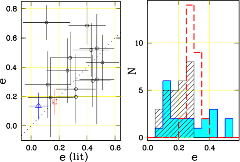
Figure 12: Comparison of our results with data from the literature. The left panel compares ellipticities of selected clusters. The clusters from Chen et al. (2004) are shown with open circles, the Pleiades (Raboud & Mermilliod 1998a) with a red square, and Praesepe (Raboud & Mermilliod 1998b) with a blue triangle. The dotted line is the bisector. Right panel: comparison of distributions with $e$ for 21 clusters with $t>50$ Myr within the Galactic longitude range $144^{\circ}...250^{\circ}$ of Chen et al. (2004) – filled histogram, and our 27 clusters within the same longitude and age ranges (hatched histogram). The dashed (red) histogram is the distribution of full models (set MC) of 27 clusters. See details in the text.

In Fig. 12 (right panel) we compare the distributions of cluster ellipticities of Chen et al. (2004) with our models (MC) and observations (OC). In order to avoid coordinate-dependent mis-interpretations, we consider only those clusters from our basic sample that are located in the same area of the sky as the clusters of the sample of Chen et al. (2004), i.e. $l=144^{\circ}\dots 250^{\circ},\,b=-18^{\circ}\dots 20^{\circ}$. We also exclude all clusters younger than 50 Myr from the comparison. The restricted samples include 21 clusters of Chen et al. (2004) and 27 of our clusters with observed and model ellipticities. Whereas N-body models forecast an average ellipticity of $e\approx 0.3$ and a narrow spread of ellipticities in this Galactic direction, our observations show a much wider distribution enhanced at smaller ellipticities ($e=0.06...0.29$). Provided that the peak in the distribution of Chen et al. (2004) data at low ellipticities ($e\approx 0.10-0.15$) is not random, we conclude that their data suffer even more from the restricted area bias than our observations do. The large spread in the data of Chen et al. (2004) can be explained by larger random errors of their ellipticities.

We briefly mention here results on the ellipticities of Galactic globular clusters. For the latter White & Shawl (1987) determined shape parameters based on the equidensity contours method from the data of Palomar and SRC Sky surveys. They find that for 99 globular cluster the average ellipticity is only $0.07\pm 0.01$, and the orientation angles are distributed randomly (because the clusters are almost round). White & Shawl (1987) point to interstellar extinction as a probable reason of such an unexpected result.

5 Conclusion

Based on a multicomponent analysis of coordinates of the most probable cluster members we have determined shape parameters of 650 Galactic open clusters. Ellipticities and orientation angles complete the list of morphological and dynamical parameters (core sizes and apparent cluster radii, indicators of mass segregation, tidal radii) which were determined and analysed in a series of previous papers (Schilbach et al. 2006; Piskunov et al. 2007, 2008a).

We have carried out high resolution N-body simulations with the specially developed $\phi$GRAPE code on the parallel GRAPE systems developed at ARI Heidelberg and MAO Kiev. The set of 27 cluster models (3 initial masses $\times$ 3 Galactocentric distances $\times$ 3 rotation parameters) with a maximum number of particles of 40404 was evolved during 1 Gyr. The cluster particles are initially distributed according to a Salpeter IMF in the mass range $0.08...8.0\leavevmode\nobreak\ m_{\odot}$. For each particle, the decision on its cluster membership is made by comparing its potential and kinetic energies.

The calculations of the apparent shape parameters of the modelled and observed clusters were carried out with the same technique. The selection of suitable models was based on initial cluster masses that were estimated from the earlier studies of our cluster sample (Piskunov et al. 2007, 2008a). This enabled us to realize a self-consistent approach for comparison of model and observed shape parameters using the data on 152 of the most populated Galactic clusters from our sample.

N-body calculations show that all the models loose more than about 50% of their initial mass during the first Gyr of the evolution due to two body encounters only. A model cluster older than $\approx 50$ Myr keeps an oblate shape, with the major axis $a$ tilted with respect to the Galactocentric radius at an angle of $\approx$30-40 degrees. The model counterparts corresponding to 152 observed clusters have an ellipticity distribution with a peak at $e\approx 0.3..0.4$, and, on average, the ellipticity becomes even larger for rotating model clusters.

However, the observed clusters show a significantly lower ellipticity, typically of about $e=0.2$. A comparison of observed cluster shapes with the detailed models allowed us to realize that lower ellipticities are only apparent. We explain this disagreement by a bias in observations due to underestimated cluster sizes $r_{2}$ based on the ASCC-2.5 data and used in the determination of cluster ellipticities. According to the models, the ellipticity of the central region of a cluster is small, it increases if outer layers are taken into account, and approaches asymptotically the largest value at 2-3 tidal radii $r_{t}$. Particles outside the tidal radius contribute negligibly to the cluster mass, however, their spatial distribution is decisive for the determination of the cluster ellipticity. Due to a relatively low density of cluster members above the background in outer cluster regions, real clusters are usually observable only within distances smaller than $r_{t}$ from the cluster centres. Though the apparent cluster sizes $r_{2}$ based on the ASCC-2.5 are twice as large as previously published in the literature, the ratio $r_{2}/r_{t}$ was found to be, on average, only 0.5 (Piskunov et al. 2008a).

In contrast, the deepness of the survey does not play such a dramatic role for the ellipticity determination. Although deeper surveys offer a possibility to identify more numerous cluster members of lower masses and, consequently, to increase the random accuracy of the ellipticity determination, this alone is not sufficient to avoid the “restricted area bias”.

We adopt the assumption of Wielen (1974, 1985) on the preferential shape and orientation of cluster ellipsoids in the Galaxy and derive simple formulae giving a relation between the apparent ellipticity and spatial location of clusters of our sample. Due to relatively high systematic and random errors in observed ellipticities, however, we could not use the present observations for estimating the parameters of the reference ellipsoid. According to N-body calculations, the cluster ellipsoid has an axes ratio of $a:b:c=1.65:1.35:1$, and it is tilted by an angle $q_{XY}\approx 30^{\circ}$ with respect to the Galactocentric radius.

In order to test the models with the real observations, the ellipticity determination for clusters must be based on sufficiently large areas (up to two to three tidal radii) around the clusters. From this point of view, equidensity methods are hardly useful to determine real cluster sizes, especially, due to a low density contrast of cluster members above the background at large distances from the cluster centres. The membership determination with kinematic and photometric criteria fits the problem better but requires surveys with higher accuracy of proper motions than it is in the ASCC-2.5.