Tachyon field in loop quantum cosmology: An example of traversable singularity

Abstract

Loop quantum cosmology (LQC) predicts a nonsingular evolution of the universe through a bounce in the high energy region. But LQC has an ambiguity about the quantization scheme. Recently, the authors in [Phys. Rev. D 77, 124008 (2008)] proposed a new quantization scheme. Similar to others, this new quantization scheme also replaces the big bang singularity with the quantum bounce. More interestingly, it introduces a quantum singularity, which is traversable. We investigate this novel dynamics quantitatively with a tachyon scalar field, which gives us a concrete example. Our result shows that our universe can evolve through the quantum singularity regularly, which is different from the classical big bang singularity. So this singularity is only a week singularity.

I Introduction

Among the candidates for a theory of quantum gravity, the non-perturbative quantum gravity develops rapidly. In recent years, as a non-perturbative quantum gravity scheme, Loop Quantum Gravity (LQG) shows more and more strength on gravitational quantization thiemann06 . LQG is rigorously constructed on the kinematical Hilbert space. Many spatial geometrical operators, such as the area, the volume and the length operator have also been constructed on this kinematical Hilbert space. The successful examples of LQG include quantized area and volume operators rovelli95 ; ashtekar97 ; ashtekar98a ; thiemann98 , a calculation of the entropy of black holes rovelli96 , Loop Quantum Cosmology (LQC) bojowald05 , etc. As a successful application of LQG to cosmology, LQC has an outstanding and interesting result—replacing the big bang spacetime singularity of cosmology with a big bounce bojowald01 . In addition, LQC also gives a quantum suppression of classical chaotic behavior near singularities in Bianchi-IX models bojowald04a ; bojowald04b . Furthermore, it has been shown that the non-perturbative modification of the matter Hamiltonian leads to a generic phase of inflation bojowald02 ; date05 ; xiong1 .

Recently the authors in Mielczarek08 proposed a new quantization scheme (we will call it $\mu_{MS}$ scheme in the following) for LQC . In this new quantization scheme, the classical big bang singularity is also replaced by a quantum bounce. The most interestingly, this new scheme introduces a novel quantum singularity. At this quantum singularity the Hubble parameter diverges, but the universe can evolve through it regularly, which is different from the case for the classical big bang singularity. In order to investigate the novel quantum singularity in this $\mu_{MS}$ scheme, we apply it to the universe filled with a tachyon field and compared the result with the classical dynamics and the $\bar{\mu}$ scheme which is presented in our previous paper xiong1 .

The organization of this paper is as follows. In Sec. II we give out the effective framework of LQC coupled with the tachyon field, and a brief review of the new quantization scheme suggested in Mielczarek08 . In addition we show some general properties of this specified effective LQC system. In Sec. III, we use the numerical method to investigate the detailed dynamics of the universe filled with the tachyon field in the $\mu_{MS}$ scheme. At the same time we compare the difference between the $\mu_{MS}$ scheme, the $\bar{\mu}$ scheme and the classical behavior. In Sec. IV we present some comments on the traversable singularity. In Sec.V we conclude and discuss our results on the $\mu_{MS}$ quantization scheme. Throughout the paper we adopt units with $c=G=\hbar=1$.

II the effective framework of LQC coupled with tachyon field

The tachyon scalar field arises in string theory Sen02 ; Sen02b , which may provide an explanation for inflation tachyon_inflation at the early epochs and could contribute to some new form of the cosmological dark energy tachyon_dark at late times. Moreover, the tachyon scalar field can also be used to interpret the dark matter causse04 . In this paper we investigate the tachyon field in the effective framework of LQC. According to Sen Sen02 , in a spatially flat FRW cosmology the Hamiltonian for the tachyon field can be written as

$$H_{\phi}(\phi,\Pi_{\phi})=a^{3}\sqrt{V^{2}(\phi)+a^{-6}\Pi_{\phi}^{2}}$$

where $\Pi_{\phi}=\frac{a^{3}V\dot{\phi}}{\sqrt{1-\dot{\phi}^{2}}}$ is the conjugate momentum for the tachyon field $\phi$, $V(\phi)$ is the potential term for the tachyon field, and $a$ is the FRW scale factor. So we have

$$-1\leq\dot{\phi}\leq 1.$$

Following our previous work xiong1 , we take a specific potential for tachyon field Sen02b in this paper,

$$V(\phi)=V_{0}e^{-\alpha\phi},$$

where $V_{0}$ is a positive constant and $\alpha$ is the tachyon mass. Similar to xiong1 , we set $V_{0}=0.82$ and $\alpha=0.5$. For the flat model of universe, the phase space of LQC is spanned by coordinates $c=\gamma\dot{a}$ and $p=a^{2}$, being the only remaining degrees of freedom after the symmetry reduction and the gauge fixing. In terms of the connection and triad, the classical Hamiltonian constraint is given by ashtekar03

$$H_{cl}=-\frac{3}{8\pi\gamma^{2}}\sqrt{p}c^{2}+H_{\phi}.$$ (1)

Considering $\bar{\mu}$ quantization scheme, the effective Hamiltonian in LQC is given by ashtekar06b

$$H_{eff,\bar{\mu}}=-\frac{3}{8\pi\gamma^{2}\bar{\mu}^{2}}\sqrt{p}\sin^{2}\left(\bar{\mu}c\right)+H_{\phi}.$$ (2)

The variable $\bar{\mu}$ corresponds to the dimensionless length of the edge of the elementary loop and is given by

$$\bar{\mu}=\xi p^{-1/2},$$ (3)

where $\xi$ is a constant ($\xi>0$) and depends on the particular scheme in the holonomy corrections. $\xi$ is given by

$$\xi^{2}=2\sqrt{3}\pi\gamma l_{p}^{2},$$ (4)

where $l_{p}$ is the Planck length. Considering the $\mu_{MS}$ quantization scheme, the effective Hamiltonian in LQC is given by Mielczarek08

$$H_{eff,\mu_{MS}}=-\frac{3}{8\pi\gamma^{2}}\frac{1-\sqrt{1-\frac{4}{3}\sin^{2}(\bar{\mu}c)}}{\frac{2}{3}\bar{\mu}^{2}}\sqrt{p}+H_{\phi}.$$ (5)

In analogy to the $\mu_{0}$ scheme and the $\bar{\mu}$ scheme, we can understand this $\mu_{MS}$ scheme as follows. We write the effective Hamiltonian as

$$H_{eff,\mu_{MS}}=-\frac{3}{8\pi\gamma^{2}\mu_{MS}^{2}}\sqrt{p}\sin^{2}\left(\mu_{MS}c\right)+H_{\phi}.$$ (6)

While $\mu_{MS}$ is given by

$$\frac{\sin^{2}\left(\mu_{MS}c\right)}{\mu_{MS}^{2}}=\frac{1-\sqrt{1-\frac{4}{3}\sin^{2}(\bar{\mu}c)}}{\frac{2}{3}\bar{\mu}^{2}},$$ (7)

with $\bar{\mu}$ determined by Eq. (3). As to the argument for the above equation we refer to Mielczarek08 . With notation of the effective energy density $\rho_{eff}$ and the effective pressure $P_{eff}$, we can write the modified Friedmann equation, modified Raychaudhuri equation and the conservation equation in the same form

$$H^{2}=\frac{8\pi}{3}\rho_{eff},$$ (8)

$$\frac{\ddot{a}}{a}=\dot{H}+H^{2}=-\frac{4\pi}{3}\left(\rho_{eff}+3P_{eff}\right),$$ (9)

$$\dot{\rho}_{eff}+3H\left(\rho_{eff}+P_{eff}\right)=0.$$ (10)

In the above equations, $H\equiv\frac{\dot{a}}{a}$ stands for the Hubble parameter; $\rho_{eff}$ and $P_{eff}$ are the effective energy density and the effective pressure, respectively. For the following three situations: the classical cosmology, the $\bar{\mu}$ scheme and the $\mu_{MS}$ scheme in LQC, we have

$$\rho_{eff,cl} = \rho_{\phi}=\frac{V}{\sqrt{1-\dot{\phi}^{2}}},$$ (11)

$$P_{eff,cl} = P_{\phi}=-V\sqrt{1-\dot{\phi}^{2}},$$ (12)

$$\rho_{eff,\bar{\mu}} = \rho_{\phi}\left(1-\frac{\rho_{\phi}}{\rho_{c}}\right),$$ (13)

$$P_{eff,\bar{\mu}} = P_{\phi}\left(1-\frac{2\rho_{\phi}}{\rho_{c}}\right)-\frac{\rho_{\phi}^{2}}{\rho_{c}},$$ (14)

$$\rho_{eff,\mu_{MS}} = \rho_{\phi}\left(1-\frac{\rho_{\phi}}{3\rho_{c}}\right)\left[\frac{3}{4}+\frac{1}{4}\left(1-\frac{2}{3}\frac{\rho_{\phi}}{\rho_{c}}\right)^{-2}\right],$$ (15)

$$P_{eff,\mu_{MS}} = \left[P_{\phi}\left(1-4\frac{\rho_{\phi}}{\rho_{c}}\right)-\frac{\rho_{\phi}^{2}}{3\rho_{c}}\right]\left[\frac{3}{4}+\frac{1}{4}\left(1-\frac{2}{3}\frac{\rho_{\phi}}{\rho_{c}}\right)^{-2}\right]$$ (16)

$$+\frac{1}{3}\left(1-\frac{\rho_{\phi}}{3\rho_{c}}\right)\left(1-\frac{2}{3}\frac{\rho_{\phi}}{\rho_{c}}\right)^{-3}\left(\frac{\rho_{\phi}^{2}}{\rho_{c}}+\frac{\rho_{\phi}P_{\phi}}{\rho_{c}}\right),$$

where $\rho_{c}=\frac{\sqrt{3}}{16\pi^{2}\gamma^{3}l_{p}^{2}}$. In the first two lines we have already used the Hamiltonian for the tachyon field and the definitions of the energy density and the pressure hossain05

$$\rho_{\phi}=\frac{H_{\phi}}{a^{3}},\ P_{\phi}=-\frac{1}{3a^{2}}\frac{\partial H_{\phi}}{\partial a}.$$ (17)

Correspondingly, we have the following evolution equations

$$classical : \ddot{\phi}=-\left(1-\dot{\phi}^{2}\right)\frac{V^{\prime}}{V}\mp 3\dot{\phi}\left(1-\dot{\phi^{2}}\right)\left[\frac{8\pi}{3}\rho_{\phi}\right]^{1/2},$$ (18)

$$\bar{\mu} : \ddot{\phi}=-\left(1-\dot{\phi}^{2}\right)\frac{V^{\prime}}{V}\mp 3\dot{\phi}\left(1-\dot{\phi^{2}}\right)\left[\frac{8\pi}{3}\rho_{\phi}\left(1-\frac{\rho_{\phi}}{\rho_{c}}\right)\right]^{1/2},$$ (19)

$$\mu_{MS} : \ddot{\phi}=-\left(1-\dot{\phi}^{2}\right)\frac{V^{\prime}}{V}$$ (20)

$$\mp 3\dot{\phi}\left(1-\dot{\phi^{2}}\right)\left\{\frac{8\pi}{3}\rho_{\phi}\left(1-\frac{\rho_{\phi}}{3\rho_{c}}\right)\left[\frac{3}{4}+\frac{1}{4}\left(1-\frac{2}{3}\frac{\rho_{\phi}}{\rho_{c}}\right)^{-2}\right]\right\}^{1/2}.$$

In the above equations, “$-$” corresponds to the expanding universe while “$+$” corresponds to the contracting universe. For the $\bar{\mu}$ scheme, the bounce happens at $\rho_{\phi}=\rho_{c}$, so we have ashtekar06a ; ashtekar06b ; xiong1

$$\rho_{\phi}=\frac{V_{0}e^{-\alpha\phi}}{\sqrt{1-\dot{\phi}^{2}}}\leq\rho_{c}.$$

For the $\mu_{MS}$ scheme, the bounce happens at $\rho_{\phi}=3\rho_{c}$, so we have Mielczarek08

$$\rho_{\phi}=\frac{V_{0}e^{-\alpha\phi}}{\sqrt{1-\dot{\phi}^{2}}}\leq 3\rho_{c}.$$

The comparison of these features are shown in Fig. 1 and 2. In the left panel of Fig. 1 we compare the different behavior of the Hubble parameter versus the energy density of the matter. The upper half corresponds to the expansion stage of the universe, and the lower half corresponds to the contraction stage. For the $\bar{\mu}$ quantization scheme, we can see clearly the bounce behavior at $\rho_{\phi}=\rho_{c}$. When $\rho_{\phi}>\rho_{c}/2$ the universe meets a superinflation phase ($\dot{H}>0$). When $\rho_{\phi}$ becomes small, the universe behaves as the standard picture. While for the $\mu_{MS}$ scheme, the bounce happens at $\rho_{\phi}=3\rho_{c}$. When $\rho_{\phi}>3\rho_{c}/2$, the universe meets a superinflation phase. In the region where $\rho_{\phi}$ is small, the Hubble parameter of the $\mu_{MS}$ scheme is smaller than the one of the standard cosmology. In this sense the universe of the $\mu_{MS}$ scheme expands slower than the universe of the standard cosmology.

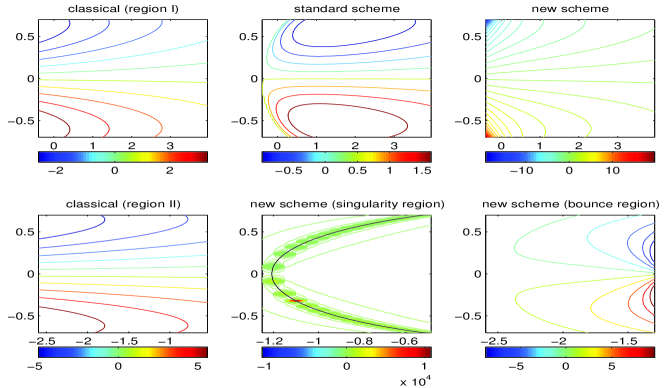
Figure 2: (color online) Comparison of $\ddot{\phi}$ in the expanding universe. The horizontal axis is $\phi$, and vertical axis is $\dot{\phi}$. The lines are contour lines for $\ddot{\phi}$. The upper row is comparison of three dynamical systems near the bounce region of the $\bar{\mu}$ quantization scheme. The lower row is comparison of the classical system and the $\mu_{MS}$ scheme. In the three subfigures of upper row we only show the admissible region for the $\bar{\mu}$ scheme, which is the common region for three dynamical systems. The lines are contour plot of $\ddot{\phi}$. The figure does not show this singularity properly due to the numerical resolution. But the envelopes of islands in this figure are true. At present, we are not clear what physical phenomena these islands will result in. Near the bounce region, the behavior of $\ddot{\phi}$ is similar to the one of the $\bar{\mu}$ scheme in its corresponding bounce region (compared middle subfigure in the upper row with the one of last subfigure in the lower row).

In Fig. 2 we compare the different behavior of $\ddot{\phi}$ in the expanding universe (taking “-” in Eqs. (18)-(20)), in the phase space, i.e., $\dot{\phi}$-$\phi$ space. Firstly, from the upper three subfigures, we can see that the quantum correction in the $\bar{\mu}$ scheme of LQC changes the amplitude of classical $\ddot{\phi}$ very small, while in contrast, the quantum correction in the $\mu_{MS}$ scheme changes this amplitude significantly. Besides, the quantum correction in the $\bar{\mu}$ scheme changes obviously the line shapes for iso-$\ddot{\phi}$, while the quantum correction in the $\mu_{MS}$ scheme changes the line shapes negligibly. This difference results from the different locations of the bounce region. In fact, the quantum effect is the strongest in the bounce region for different quantum corrections. The region shown in these three upper subfigures is near the bounce region for the $\bar{\mu}$ scheme while some far away from the bounce region of the $\mu_{MS}$ scheme. Secondly, in the lower three subfigures, we compare the quantum correction from $\mu_{MS}$ of LQC with the classical behavior. We see that the behavior of $\ddot{\phi}$ near the singularity region is changed completely. $\ddot{\phi}$ diverges when the state approaches the singularity line (the contour line of $\rho_{\phi}=\frac{3}{2}\rho_{c}$) except for one point $\left(\phi,\dot{\phi}\right)=\left(-\frac{1}{\alpha}\ln{\frac{3\rho_{c}}{2V_{0}}},0\right)$ where $\ddot{\phi}=\alpha$. Yet near the bounce region, the behavior of $\ddot{\phi}$ is similar to the one of the $\bar{\mu}$ scheme in its corresponding bounce region.

III quantitative analysis of the cosmological dynamics coupled with tachyon field

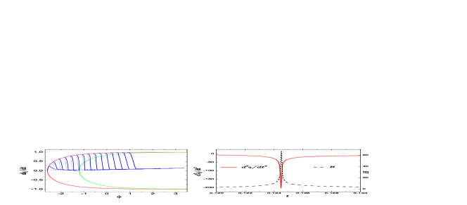
Figure 3: (color online) Lept panel, comparing of the dynamical trajectories for the classical (dotted lines) and the $\mu_{MS}$ quantization scheme (solid lines) under the expanding universe scenario in $\dot{\phi}-\phi$ space. The left “C” shape line is the boundary of admissible states for the $\mu_{MS}$ scheme, which is also the iso line of $\rho_{\phi}=3\rho_{c}$. The right “C” shape line corresponds to the singularity (the iso line of $\rho_{\phi}=1.5\rho_{c}$) for the $\mu_{MS}$ scheme, which is also the interface for hyper-inflationary and deflationary states. Right panel, the concrete example of the dynamical behavior of $\ddot{\phi}$ and the Hubble parameter $H$ near singularity for the $\mu_{MS}$ quantization scheme, which corresponds to any line which passes through the singularity for the $\mu_{MS}$ scheme in the left panel. The behavior of other ones are similar on the singularity. The solid line shows behavior of $\ddot{\phi}$, while the dotted line shows behavior of the Hubble parameter $H=\frac{\dot{a}}{a}$. This subfigure is a blow-up near singularity.

In the original paper Mielczarek08 , the authors provided qualitative analysis of the dynamics for LQC in the $\mu_{MS}$ scheme. Take the advantage of the specific model of the universe coupled with the tachyon field, we can investigate this dynamics for LQC quantitatively, and compare the difference between the classical, the $\bar{\mu}$ scheme and the $\mu_{MS}$ scheme dynamics. We solve the equations (18), (19) and (20) with the Rung-Kutta subroutine. The result is presented in Fig. 3.

For the $\mu_{MS}$ scheme, the difference between the classical and the quantum behaviors is more explicit in the region between the bouncing boundary and the singularity line. While the difference in the region on the right-hand side of singularity is negligible. Note that the admissible states for the $\bar{\mu}$ scheme all locate in this region. So we can imagine that the difference between the $\mu_{MS}$ scheme and the $\bar{\mu}$ scheme is nothing but the difference between the classical one and the $\bar{\mu}$ one, which is presented in Figs. 1 and 2 of our previous paper xiong1 . Near the bounce region, the quantum behavior is similar for both the $\bar{\mu}$ scheme and the $\mu_{MS}$ scheme. Certainly, this behavior emerges at different places in $\dot{\phi}$-$\phi$ space for the $\bar{\mu}$ scheme and the $\mu_{MS}$ scheme respectively. Near the singularity region, there is not special respects for the quantum evolution in the $\dot{\phi}$-$\phi$ space, except that the quantum trajectories are much steeper than the classical ones. This steeper behavior is resulted from the singularity behavior of the quantum dynamics which makes $\ddot{\phi}$ much larger than the original classical ones. From the right panel of Fig.3, we can see that both the hyper-inflationary and deflationary phases of the universe emerged clearly. The universe expands increasingly faster before singularity untill the acceleration becomes infinity. This stage corresponds to the hyper-inflationary phase for the universe. After this singularity, the universe expands more and more slowly. The behavior comes back to the classical one sami02 ; guo03 quickly. This stage is the deflationary phase for the universe.

IV Comments on the traversable singularity

As a dynamical system, (20) is singular when $\rho_{\phi}=3\rho_{c}/2$, which corresponds to the right “C” shaped curve of the left panel of Fig.  3. That means that the dynamical system is only defined in two separated regions. One is the region between the left “C” shaped line and the right “C” shaped line, and the another is the region on the right-hand side of the right “C” shaped line. Then a question arises naturally–does the numerical behavior traversing the separated “C” shaped line make sense or is it only a numerical cheating ? If we consider these two regions separately the dynamical system is well defined in the sense of the Cauchy uniqueness theorem. The orbits in the phase space $\phi$-$\dot{\phi}$ are smooth. Taking the phase space as $R^{2}$, these orbits are smooth curves. So these smooth curves have proper limit points on the separated “C” shaped line. From the numerical solutions shown in Fig.  3, we can see that the different orbits have different limit points on the “C” shaped line. This is because the vector flow generating the trajectories (on the $\phi$-$\dot{\phi}$ plane) has well-defined directions (vertical) at the singularity, which means the trajectories cannot intersect there. Then it is natural to join the two orbits in the two separated regions with the same limit points. In this way we get a well-defined dynamical system in the total region which lies on the right-hand side of the left “C” shaped line. We can expect the numerical solution with the Rung-Kutta method will converge to this solution (we also performed numerical integrations starting from both sides towards the singular point and obtained the same result). So the numerical result presented in the above sections does make sense.

In the following, we come back to the spacetime to check the property of this traversable singularity. Corresponding to the two separated regions of phase space $\phi$-$\dot{\phi}$, the scale factor $a$ can be determined by $\phi$ and $\dot{\phi}$ through

$$a(\phi,\dot{\phi})=(\rho_{\phi}/H_{\phi})^{1/3}$$ (21)

which is a smooth function of $\phi$ and $\dot{\phi}$. Therefore, the two spacetime regions of the universe corresponding to these two regions is smooth. When the universe evolves to $\rho_{\phi}=3\rho_{c}/2$, $a$ is also well defined through (21). That implies that the whole spacetime of the universe is well defined through joining the above mentioned two regions together by the well-defined $a$ at $\rho_{\phi}=3\rho_{c}/2$. But since $\ddot{\phi}$ is singular there, $\dot{a}$ is also singular there, which makes the spacetime of the universe unsmooth. In this sense the spatial slice corresponding to this special universe time is a traversable singularity of the spacetime.

According to ellis77 ; tipler77 ; krolak88 ; seifert77 , singularities can be classified into strong and weak types. A singularity is strong if the tidal forces cause complete destruction of the objects irrespective of their physical characteristics, whereas a singularity is considered weak if the tidal forces are not strong enough to forbid the passage of objects. In this classification the singularity discussed here is only a weak singularity. As to the cosmological singularities, they can be classified in more details with the triplet of variables ($a,\rho,P$) nojiri05 ; cattoen05 ; fernandez06 ; singh09 : Big bang and Big Crunch ($a=0$, $\rho$ and curvature invariants diverge at a finite proper time); Big Rip or type I singularity ($a$, $\rho$, $P$ and curvature invariants diverge at a finite proper time); Sudden or type II singularity ($a$ and $\rho$ are finite while $P$ diverges); type III singularity ($a$ is finite while $\rho$ and $P$ diverge); type IV singularity ($a$, $\rho$, $P$ and the curvature invariants are finite while the curvature derivatives diverge). For the singularity discussed in this paper, $a$, $\rho$ and $P$ are all finite because of the regularity of $\phi$ and $\dot{\phi}$ at the singularity. But the Ricci curvature invariant,

$$R=6(H^{2}+\frac{\ddot{a}}{a}),$$ (22)

diverges at the singularity. So the singularity here does not fall in any type of above clarification. But it is more similar to type IV singularity than to the other types.

V discussion and conclusion

In the classical cosmology our universe has a big bang singularity. All physical laws break down there. LQC replaces this singularity with a quantum bounce and the universe can evolve through the bounce point regularly. Considering the quantum ambiguity of quantization scheme in LQC, the authors in Mielczarek08 proposed a new scheme. In addition to the quantum bounce, a novel quantum singularity emerges in this new scheme. The quantum singularity is different from the big bang singularity and is traversable, although the Hubble parameter diverges at this singularity. In this paper, we follow our previous work xiong1 to investigate this novel dynamics with the tachyon scalar field in the framework of the effective LQC. We analyze the evolution of the tachyon field with an exponential potential in the context of LQC, and obviously, any other choice of potential can lead to the similar result.

In the high energy region (approaching the critical density $\rho_{c}$), LQC in the new quantization scheme greatly modifies the classical FRW cosmology and predicts a nonsingular bounce at density $3\rho_{c}$, which is located at a different density region compared with the $\bar{\mu}$ quantization scheme. In addition, besides this quantum bounce, this new quantization scheme also introduces a quantum singularity, which emerges at density $1.5\rho_{c}$. At this quantum singularity the Hubble parameter diverges. But this singularity is different from the classical one. The universe can evolve through this quantum singularity regularly. Different from the $\bar{\mu}$ scheme, the dynamics of the new quantization scheme will deviates from the classical one even in a small energy density region (see Fig. 1).

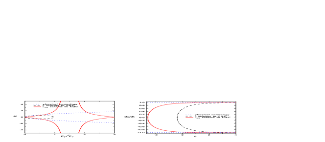
Figure 1: (color online) The dotted line, dashed line and solid line correspond to the classical, the $\bar{\mu}$ scheme and the $\mu_{MS}$ scheme dynamics respectively. Left panel: Hubble parameter versus the energy density of matter. When $\rho_{\phi}\ll 1$, the quantum correction becomes negligible in the $\bar{\mu}$ scheme, i.e., the behavior of universe goes back to classical one. But for the $\mu_{MS}$ the quantum correction is strong even when $\rho_{\phi}\ll 1$. Right panel: The phase portrait for all admissible $\phi$ and $\dot{\phi}$ and the graph shows the region boundary. These boundaries are nothing but the contour lines of $\rho_{\phi}$ in $\dot{\phi}-\phi$ space. The dashed line, dotted line and solid line correspond to $\infty$, $3\rho_{c}$ and $\rho_{c}$ respectively. The admissible states for classical system are between the two dashed lines. The admissible states for quantum system are the right part of the corresponding lines.

- (1) T. Thiemann, Mordern Canonical Quantum General Relativity, (Cambridge University Press, 2006); arXiv: gr-qc/0110034.
- (2) C. Rovelli and L. Smolin, Nucl. Phys. B 442, 593 (1995).
- (3) A. Ashtekar and J. Lewandowski, Class. Quant. Grav. 14, A55 (1997).
- (4) A. Ashtekar and J. Lewandowski, Adv. Theor. Math. Phys. 1, 388 (1998).
- (5) T. Thiemann, J. Math. Phys. 39, 3372 (1998).
- (6) C. Rovelli, Phys. Rev. Lett. 77, 3288 (1996).
- (7) M. Bojowald, Living Rev. Relativity lrr-2008-4.
- (8) M. Bojowald, Phys. Rev. Lett. 86, 5227 (2001).
- (9) M. Bojowald, G. Date, Phys. Rev. Lett. 92, 071302 (2004).
- (10) M. Bojowald, Class. Quantum Grav. 21, 3541 (2004).
- (11) M. Bojowald, Phys. Rev. Lett. 89, 261301 (2002).
- (12) G. Date and G. Hossain, Phys. Rev. Lett. 94, 011301 (2005).
- (13) Hua-Hui Xiong and Jian-Yang Zhu, Phys. Rev. D 75, 084023 (2007).
- (14) J. Mielczarek and M.Szydlowski, Phys. Rev. D 77, 124008 (2008).
- (15) A. Sen, J. High Energy Phys. 04 (2002) 048; 07 (2002) 065.
- (16) A. Sen, Mod. Phys. Lett. A 17, 1797 (2002).
- (17) G. Gibbons, Phys. Lett. B 537, 1 (2002); A. Feinstein, Phys. Rev. D 66, 063511 (2002); T. Padmanabhan, Phys. Rev. D 66, 021301(R) (2002); M. Sami, D. Chingangham, and T. Qureshi, Phys. Rev. D 66, 043530 (2002); A. Frolov, L. Kofman, and A. Linde, Phys. Lett. B 545, 8 (2002); S. Sugimoto and S. Terashima, J. High Energy Phys. 07, 025 (2002).
- (18) A. Riess et al., Astron. J. 116, 1009 (1998); S. Perlmutter et al., Astrophys. J. 517, 565 (1998); G. Efstathiou et al., Mon. Not. R. Astron. Soc. 330, L29 (2002).
- (19) M. Causse, arXiv: astro-ph/0312206v2.
- (20) A. Ashtekar, M. Bojowald, and Lewandowski, Adv. Theor. Math. Phys. 7, 233 (2003).
- (21) A. Ashtekar, T. Pawlowski, and P. Singh, Phys. Rev. D 74, 084003 (2006).
- (22) G. Hossain, Classical Quantum Gravity 22, 2653 (2005).
- (23) A. Ashtekar, T. Pawlowski, and P. Singh, Phys. Rev. D 73, 124038 (2006).
- (24) M. Sami, P. Chingangbam, and T. Qureshi, Phys. Rev. D 66, 043530 (2002).
- (25) Z. Guo, Y. Piao, and R. Cai, Phys. Rev. D 68, 043508 (2003).
- (26) G. Ellis, and B. Schmidt, Gen. Rel. Grav. 8, 915 (1977).
- (27) F. Tipler, Phys Lett. A 64, 8 (1977).
- (28) A. Krolak, Class. Quantum Grav. 3, 267 (1988).
- (29) H. Seifert, “Causal structure of singularities”, in Differential Geometric Methods in Mathematical Physics, Lecture notes in Mathematics, Springer (1977).
- (30) S. Nojiri, S. Odintsov, and S. Tsujikawa, Phys. Rev. D 71, 063004 (2005).
- (31) C. Cattoen, and M. Visser, Class. Quantum Grav. 22, 4913 (2005).
- (32) L. Fernandez-Jambrina, and R. Lazkoz, Phys. Rev. D 74, 064030 (2006).
- (33) P. Singh, arXiv: 0901.2750v1.