Could the photon dispersion relation be non-linear ?

Abstract.

The free photon dispersion relation is a reference quantity for high precision tests of Lorentz Invariance. We first outline theoretical approaches to a conceivable Lorentz Invariance Violation (LIV). Next we address phenomenological tests based on the propagation of cosmic rays, in particular in Gamma Ray Bursts (GRBs). As a specific concept, which could imply LIV, we then focus on field theory in a non-commutative (NC) space, and we present non-perturbative results for the dispersion relation of the NC photon.

1. Lorentz Invariance Violation (LIV)

Lorentz Invariance (LI) plays a central rôle in relativity: it holds as a global symmetry in Special Relativity Theory, and as a local symmetry in General Relativity Theory. We refer to the former in order to be able to describe particle physics in terms of quantum field theory, where a field $\Phi$ (scalar, vector, tensor or spinor) is transformed globally in some representation $D$ of the Lorentz group $SO(1,3)$,

$$\Phi(x)\to U(\Lambda)^{\dagger}\Phi(x)U(\Lambda)=D(\Lambda)\Phi(\Lambda^{-1}x)\ ,\quad U~{}{\rm unitary}\ ,\quad\Lambda\in SO(1,3)\ .$$ (1)

If a local field theory obeys LI, then it is also CPT invariant [2]. If LI is broken, CPT may be intact or not. If, however, CPT is broken, then a LI Violation (LIV) is inevitable [3]. Therefore LI can be probed indirectly by testing CPT predictions, such as the equivalence of the mass and magnetic moment of particles and their antiparticles. In particular the masses of $K^{0}$ and $\bar{K}^{0}$ coincide to a relative precision $<8\cdot 10^{-19}$ [4].

Specific direct LI tests are even more stringent. In the framework of the Standard Model Extension (SME) [5], local terms are added to the Standard Model Lagrangian, which can cause a spontaneous LIV, e.g.

$${\cal L}={\rm i}\bar{\psi}\gamma_{\mu}\partial^{\mu}\psi-g\bar{\psi}\phi\psi-{\rm i}\bar{\psi}(g^{\prime}G_{\mu\nu}+g^{\prime\prime}H_{\mu\nu}\gamma_{5})\gamma^{\mu}\partial^{\nu}\psi+\dots$$ (2)

Spontaneous Symmetry Breaking (SSB) of the Higgs field $\phi\in{\kern 2.5pt\sf{C}\kern-4.49997pt\sf{{\small{I}}}\kern 4.49997pt\kern-2.5pt}^{2}$ leads to the fermion mass. In analogy the new tensor fields $G$ and $H$ may also undergo SSB, which affects LI (unlike the SSB of the Higgs field). For a simple change of the observers frame, $G$ and $H$ are transformed as well, so that ${\cal L}$ remains invariant; but the fermion $\psi$ perceives them as an invariant background. LIV is then manifest for instance through a modified fermion dispersion relation, depending on the Yukawa-type couplings $g^{\prime}$, $g^{\prime\prime}$. Kostelecký et al. identified more than 100 parameters of this kind (for a review, see Ref. [6]), which are claimed to be compatible with the usual properties of the Standard Model except for LI (and in part CPT) [7]. This corresponds to a low energy expansion, after lifting the usual LI condition. This collaboration interprets the photon as a Nambu-Goldstone boson [8]. All LIV parameters emerging in this framework are experimentally bounded by $O(10^{-27})$ (in a dimensionless form, which factors out the Planck scale) [9]. If some of these parameters are non-zero, they still allow for sizable LIV effects at tremendous energies, though this scenario poses a severe hierarchy problem [10].

In an effective approach, Coleman and Glashow considered Maximal Attainable Velocities (MAVs, attained in the high energy limit), which could slightly differ from the speed of light, depending on the particle type [11]. They were most interested in the impact on cosmic rays (which attain the highest energies in the Universe). In particular the prediction that proton rays cannot exceed the Greisen-Zatsepin-Kuz’min (GZK) energy of $E_{\rm GZK}\approx 6\cdot 10^{19}~{}{\rm eV}$ over a distance of more than $\sim 100~{}{\rm Mpc}$ in the Cosmic Microwave Background (CMB) (mainly due to photopion production via a $\Delta$-resonance) could be evaded by tiny MAV differences. However, recent observations favour the validity of the GZK energy cutoff [12]: up to $E_{\rm GZK}$ the cosmic ray flux follows closely a behaviour $\propto E^{-2.7}$, but beyond $E_{\rm GZK}$ there is an extra suppression compared to this power law. This suggests that LI holds even under boosts of Lorentz factors like $\gamma=E_{\rm GZK}/m_{\rm proton}\sim 10^{11}$, i.e. 6 orders of magnitude beyond the $\gamma$-factors accessible in laboratories, which further constrains the MAV differences [13].

This issue is reviewed in Ref. [14], covering theoretical and phenomenological aspects and the current status, along with MAV effects in cosmic rays with respect to decays, Čerenkov radiation and neutrino oscillation [15] (these effects were addressed already in Ref. [11], and reviewed earlier in Ref. [16]).

2. Cosmic $\gamma$-rays

The highest energies in cosmic $\gamma$-rays have been observed around $E_{\gamma}\sim 50~{}{\rm TeV}$. They were emitted from the Crab Nebula [17] (a remnant of a supernova of the year 1054, at a distance of $2~{}{\rm kpc}$). With certain assumptions about the origin of these rays (synchrotron radiation of high energy electrons and positrons, followed by powerful inverse Compton scattering) one obtains stringent LIV constraints [16].

The most energetic $\gamma$-rays reaching us from outside our galaxy originate from blazars, a subset of the Active Galactic Nuclei. Two prominent blazars are denoted as Markarian 501 and 421 at distances of about $157~{}{\rm Mpc}$ and $110~{}{\rm Mpc}$, which had emitted photons that arrived at Earth with $E_{\gamma}\sim 20~{}{\rm TeV}$ [18] resp. $E_{\gamma}\sim 10~{}{\rm TeV}$ [19]. These multi-TeV $\gamma$-rays have been considered a puzzle similar to the GZK cutoff (which seemed to disagree with the data in the 20^th century): they give rise to the creation of electron/positron pairs in the CMB , which can perform inverse Compton scattering on further CMB photons. This leads to a cascade of high energy photons, which are attenuated in this way. The penetration depth of these cascades in the CMB, above certain energy thresholds, is reviewed for instance in Ref. [20]: it is sensitive to details of the extragalactic magnetic fields and the radio background, which are not known precisely. In analogy to the GZK energy cutoff, also here LIV effects — and in particular MAV differences — have been proposed as an explanation for the possibly puzzling $\gamma$-radiation from blazars [21]. However, also in this case it is not clear if they really represent a puzzle — e.g. the analysis in Refs. [22] suggest that their understanding does not require new physics.

Since 1967 we also know about the existence of Gamma Ray Bursts (GRBs), which are emitted in powerful eruptions. Temporarily they yield the brightest spots in the sky. Typically they last for a few seconds or minutes, and they involve photons in the energy range $E_{\gamma}\approx(10^{4}\dots 10^{8})~{}{\rm eV}$. About their origin we only have speculations, such as the merger of black holes or neutron stars, along with fireball shock models for the GRB generation. In any case their existence is suggestive for a high precision test of the photon dispersion relation, which represents a purely kinematic facet of LI [23]. A deviation from the linear dispersion relation, i.e. a photon group velocity $v_{\gamma}(E_{\gamma})\neq const.\,$, can be obtained most simply by introducing a photon mass $m_{\gamma}>0$ (through a modified Higgs mechanism, keeping the photon MAV unaltered). However, the bound based on laboratory experiments, $m_{\gamma}<10^{-18}~{}{\rm eV}$ [4], is so tiny that its impact would still not be detectable in GRBs [23]. Hence this approach is not attractive in this context and we return to $m_{\gamma}=0$.

Instead we switch to the simple effective ansatz (with the photon speed $c=1$ attained at low $E_{\gamma}$)

$$v_{\gamma}\simeq 1-\frac{E_{\gamma}}{M}\ ,$$ (3)

where $M$ is a very heavy mass parameter (which could emerge from some unspecified “quantum gravity foam”), and we consider only $O(E_{\gamma}/M)$. Ref. [24] confronted this ansatz with the data of 35 GRBs measured from three satellites, and observed that photons with higher energy tend to arrive earlier. They parametrised the observed time delay $\Delta t$ between energy channels, which differ by $\Delta E$, as

$$\frac{\Delta t}{1+z}=d_{\rm source}+a_{\rm LIV}\,K(z)\ ,\quad a_{\rm LIV}:=\frac{\Delta E}{H_{0}M}\ ,\quad H_{0}~{}:~{}{\rm Hubble~{}parameter},~{}z~{}:~{}{\rm redshift}\ .\quad$$ (4)

The parameter $d_{\rm source}$ captures a possible relative delay already at the source, and $K(z)$ is a function of the redshift, which is derived in Ref. [24]. The question is now whether or not the data are compatible with a vanishing LIV parameter. Fig. 1 (on the left) shows that they do certainly not rule out $a_{\rm LIV}=0$, although the best linear fit has a slight slope. The plot on the right specifies the windows for the parameters $d_{\rm source}$ and $a_{\rm LIV}$ with 68 % resp. 95 % confidence level (C.L.). The observation that $a_{\rm LIV}$ cannot deviate much from zero implies [24]

$$|M|>1.4\cdot 10^{25}~{}{\rm eV}\approx 0.001\ M_{\rm Planck}\qquad{\rm(with~{}95~{}\%~{}C.L.)\ .}$$ (5)

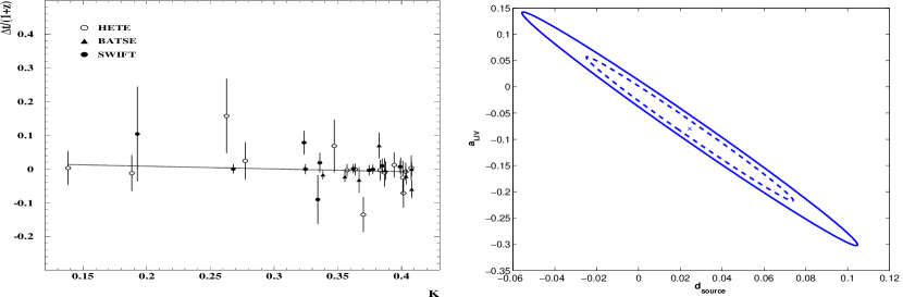
Figure 1. Evaluation of the parameters in eq. (4) from GRB data of three satellites. The plot on the left shows the left-hand-side of eq. (4) against the function $K(z)$. The plot on the right illustrates the resulting bounds for the parameters $d_{\rm source}$ (relative delay at the source) and $a_{\rm LIV}$ (LIV effects) with 68 % resp. 95 % C.L. (plots adapted from Ref. [24]).

This result appears robust due to the large data set considered. Similar studies based on single GRBs or blazar flares (again involving Markarian 501) did not report evidence for LIV either, and derived bounds for $|M|$ even up to $O(0.01)\cdot M_{\rm Planck}$ [25].

As another purely kinematic effect — which does not require any assumptions about the interactions in a LIV modified form of QED — there could be vacuum birefringence, if $v_{\gamma}$ is slightly helicity dependent,

$$v_{\gamma}^{\pm}(k)=1\pm\frac{k}{2M_{\rm h}}\qquad(k=|\vec{k}\,|~{}:~{}{\rm momentum},~{}M_{\rm h}~{}:~{}{\rm heavy~{}mass},~{}\pm~{}:~{}{\rm helicities})\ .$$ (6)

In this case linearly polarised light should be depolarised completely after a long enough time of flight. However, cosmic $\gamma$-rays from quasars at a distance of $300~{}{\rm Mpc}$, with wave lengths of $(400\dots 800)~{}{\rm nm}$ were observed, essentially with a linear polarisation (less than $10^{\circ}$ deviation from the polarisation plane) [26]. This implies for that LIV scenario even a strongly trans-Planckian bound: $|M_{\rm h}|>10^{4}\,M_{\rm Planck}$ [27].

Still better precision is expected soon from GRB and blazar flare photons with $E_{\gamma}\approx 8~{}{\rm keV}\dots 300~{}{\rm GeV}$, to be detected by the Fermi Gamma-ray Space Telescope [28], which arrived in orbit in June 2008. In addition the Chinese-French Space-based multi-band astronomical Variable Objects Monitor mission (SVOM) [29] plans to monitor about 80 GRBs a year, starting in 2013.

Also the subjects of this section are reviewed more extensively in Refs. [16, 14].

3. $U(1)$ gauge theory in a non-commutative (NC) plane

We now address another theoretical concept for LIV, which is fundamentally different from the low energy effective approaches [5, 11] that we referred to in Section 1. We first consider a Euclidean plane given by Hermitian coordinate operators $\hat{x}_{1},\,\hat{x}_{2}$, which do not commute. This yields a purely spatial uncertainty relation,

$$[\hat{x}_{\mu},\hat{x}_{\nu}]={\rm i}\theta\epsilon_{\mu\nu}\ ,\quad\Delta x_{1}\cdot\Delta x_{2}\mathop{\raise 1.29167pt\hbox{$>$\kern-7.5pt\raise-4.73611pt\hbox{$\sim$}}}\frac{1}{2}|\theta|\ .$$ (7)

Here we assume $\theta=const.$ (which can be generalised, of course). $\sqrt{|\theta|}$ now represents a kind of “minimal length”, as a new constant of Nature, like the parameters $1/M$ or $1/M_{\rm h}$ in Section 2. It might have an interpretation as the event horizon of a mini black hole in a (hypothetical) attempt to measure distances of $O(L_{\rm Planck})$ (which would require a tremendous energy density) [30]. Field theory on such a space is necessarily non-local over this range. This gives rise to the mixing between UV and IR divergences, which makes perturbation theory mysterious (for a review, see e.g. Ref. [31] and references therein).

Here we refer to a fully non-perturbative approach, which starts by introducing a lattice structure. Let the spectra of $\hat{x}_{1}$ and $\hat{x}_{2}$ be discrete multiples of some “lattice spacing” $a$ (although there are no sharp lattice sites, since $\hat{x}_{1}$, $\hat{x}_{2}$ cannot be diagonalised simultaneously). On the other hand, the momentum components $k_{1},\,k_{2}$ commute, and they obey the usual periodicity over the Brillouin zone,

$$e^{{\rm i}k_{\mu}\hat{x}_{\mu}}=e^{{\rm i}(k_{\mu}+2\pi/a)\hat{x}_{\mu}}\quad\Rightarrow\quad\hat{1}\!\!1=e^{{\rm i}(k_{\mu}+2\pi/a)\hat{x}_{\mu}}\ e^{-{\rm i}k_{\nu}\hat{x}_{\nu}}=\hat{1}\!\!1\ e^{{\rm i}\pi\theta(k_{2}-k_{1})/a}\quad\Rightarrow\quad\frac{\theta}{2a}k_{\mu}\in Z\!\!\!Z\ .\qquad$$

For fixed parameters $\theta$ and $a$ the momenta turn out to be discrete, i.e. the lattice must be periodic. Let us assume periodicity over a $N\times N$ lattice, hence the $k_{\mu}$ are integer multiples of $2\pi/(aN)$, and from the computation above we infer

$$\theta=\frac{1}{\pi}Na^{2}\ .$$ (8)

In our studies we were therefore interested in the Double Scaling Limit (DSL), which takes $a\to 0$ and $N\to\infty$, while keeping $Na^{2}=const.$ This simultaneous UV and IR limit leads to a continuous NC plane of infinite extent. The necessity to link these limits is related to the UV/IR mixing mentioned above. In other regularisation schemes it is less obvious how to achieve this delicate balance.

It is equivalent to return to coordinates $x_{\mu}$, but perform all field multiplications by a star product, e.g.

$$\phi(x)\star\psi(x):=\phi(x)\exp\Big{(}\frac{\rm i}{2}\mathop{\raise 6.02773pt\hbox{$\leftarrow$\kern-7.5pt\raise-6.02773pt\hbox{$\partial$}}}\ \!\!\!_{\mu}\,\theta\,\epsilon_{\mu\nu}\!\mathop{\raise 6.02773pt\hbox{$\rightarrow$\kern-7.5pt\raise-6.02773pt\hbox{$\partial$}}}\ \!\!\!_{\nu}\Big{)}\psi(x)\ .$$ (9)

Thus the NC $U(1)$ pure gauge action takes the star-gauge invariant form

$$S[A]=\frac{1}{2}\int d^{2}x\,F_{\mu\nu}\star F_{\mu\nu}\ ,\quad F_{\mu\nu}=\partial_{\mu}A_{\nu}-\partial_{\nu}A_{\mu}+{\rm i}g(A_{\mu}\star A_{\nu}-A_{\nu}\star A_{\mu})\ ,$$ (10)

which involves a Yang-Mills term. Its lattice discretisation does not appear simulation-friendly; note that compact link variables would have to be star-unitary. However, there is an exact map onto a matrix model in one point — the twisted Eguchi-Kawai model [32] — which is Morita equivalent [33]. This renders simulations feasible, and it also provides a sound definition of Wilson loops. These Wilson loops are complex in general, but the lattice action is real positive, since it sums over both plaquette orientations.

Our Monte Carlo simulations — using a heat-bath algorithm — revealed the following features [34]: at small area the Wilson loops $\langle W\rangle$ of all shapes are real and they follow an area law behaviour. At large area, however, a complex phase sets in, which obeys for many shapes the simple relation ${\rm arg}\langle W\rangle={\rm area}/\theta$. If we formally identify $1/\theta$ with a magnetic field across the plane, then this is the behaviour of the Aharonov-Bohm effect. This identification can be conjectured on tree level, and it has been used extensively in the literature; for instance, it is inherent in the Seiberg-Witten map [35]. In the case discussed above, however, this relation only shows up as a non-perturbative effect.

Moreover the Wilson loops of large area were observed to be shape dependent, so the symmetry under Area Preserving Diffeomorphisms is broken, including the subgroup of linear unimodular transformations, $SL(2,R)$ [36]. That symmetry was a corner stone in the solution of Yang-Mills theories in a commutative plane. We conclude that the same technique cannot be applied in the NC plane, so an analytical solution would be difficult, but the system may have a rich structure.

4. The fate of the non-commutative photon

It is straightforward to extend action (10) to higher dimensions and any $U(n)$ gauge group in the fundamental representation, but the formulation of $SU(N)$ gauge theories in NC spaces fails. Therefore 4d NC $U(1)$ gauge theory is appropriate to investigate a link to particle phenomenology.

On the perturbative side, the 1-loop calculation of the effective potential suggests a photon dispersion relation of the form [37]

$$E^{2}=\vec{p}^{\,2}+C\,\frac{g^{2}}{p\circ p}\ ,\quad p\circ p:=-\Theta^{\mu\nu}p_{\nu}\Theta_{\mu}^{\ \ \sigma}p_{\sigma}\geq 0\ ,\quad(\ C=const.,\ \ \Theta^{\mu\nu}=-{\rm i}\,[\hat{x}^{\mu},\hat{x}^{\nu}]\ )\ ,\quad$$ (11)

which contains an IR divergence at finite $\Theta$. Moreover we see that the transition to a vanishing non-commutativity tensor, $\Theta\to 0$, is not smooth (which invalidates an expansion in small $\|\Theta\|$). Therefore one could even feel tempted to claim a lower bound for $\|\Theta\|$ — if it is non-zero — from the fact that no deviation from the linear dispersion has been observed down to small photon momenta [38].

However, the situation becomes even more dramatic due to the observation that the above 1-loop correction is actually negative, $C=-2/\pi^{2}$ [39]. This looks worrisome indeed: the theory seems to be IR unstable. Without a ground state the system does hardly have a physical interpretation. The negative IR divergence is avoided in a supersymmetric version, but here we are interested in the NC photon without a SUSY partner. We addressed the issue of its stability in a fully non-perturbative study [41].

To this end we considered a Euclidean space consisting of a commutative and a NC plane. The former contains the Euclidean time. This is essential in order to preserve reflection positivity as one of the Osterwalder-Schrader axioms, which are required for the transition to Minkowski signature. Once time is commutative, non-commutativity can be restricted to one plane by means of rotations. This setting is the safest NC formulation beyond perturbation theory, and it can be viewed as minimal non-commutativity; there is again just one non-commutativity parameter $\theta$, as in eq. (7).

We regularise the commutative plane by a standard $L\times L$ lattice, and the NC plane with an $N\times N$ lattice ($L\approx N$), which is again mapped onto $N\times N$ matrices in the twisted Eguchi-Kawai model. The first goal in our numerical study [41] was the identification of a DSL. The results for a set of observables (Wilson loops and lines and their 2-point functions, matrix spectra as coordinates of a dynamically generated geometry) stabilised to a good approximation if different $N$ and $\beta\propto 1/g^{2}$ were tuned as

$$N/\beta^{2}=const.\qquad\Rightarrow\qquad a\propto 1/\beta\qquad{\rm and}\qquad\theta\propto N/\beta^{2}\ .$$ (12)

As an example we show in Fig. 2 the real part of square shaped Wilson loops in different planes, at a fixed ratio $N/\beta^{2}=20$. In the commutative plane and in the mixed planes $\langle W\rangle$ is real due to reflection symmetry on the commutative axes. In the NC plane we see an oscillating behaviour of the real part at large area, which is due to a rotating complex phase, similar to the 2d case [34] that we described in Section 3.

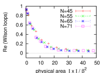
Figure 2. Wilson loops measured in NC QED₄ at $N/\beta^{2}=20$ in the commutative plane, a mixed plane and the NC plane (from left to right). In the first two planes $\langle W\rangle$ is real, whereas the oscillation of $\,{\rm Re}\,\langle W\rangle\,$ in the NC plane is due to a rotating complex phase (similar to NC QED₂ [34]).

The next goal was the exploration of the phase diagram. For this purpose we measured expectation values of open Wilson lines $P_{\mu}(n)$ in the NC plane, with a length $\Theta_{\mu\nu}p_{\nu}=na\hat{\mu}$ of a few lattice spacings ($|\hat{\mu}|=1,\ n\in\!{\kern 2.5pt\sf{N}\kern-8.00003pt\sf{I}\kern 8.00003pt\kern-2.5pt}$). The $P_{\mu}(n)$ are gauge invariant in NC space; note that star-gauge transformations are non-local themselves. Since these open Wilson lines carry finite momentum, they are suitable order parameters to detect the spontaneous breaking of translation symmetry. Results for $N=15,\,25$ and $35$ are shown in Fig. 3.

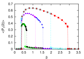
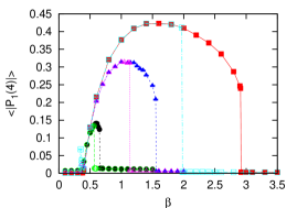
Figure 3. The expectation values of open Wilson lines of length $2$ and $4$ lattice spacings (on the left/right) for $N=15,\ 25$ and $35$ (curves connecting bullets, triangles and squares, with hysteresis at the transition to the weak coupling phase). At intermediate gauge coupling we discovered a phase of spontaneously broken translation symmetry.

Translation symmetry is intact at strong and at weak gauge coupling, in agreement with the corresponding expansions, but it is broken at intermediate coupling. This effect is purely non-perturbative; it was not visible in analytical studies. The transition strong/moderate coupling occurs at $\beta\approx 0.35$ (for any $N$), whereas the transition moderate/weak coupling roughly follows a behaviour $\beta\propto N^{2}$ (that phase transition is of first order, as we see in Fig. 3 from the hysteresis). The existence of a broken symmetry phase at moderate coupling was also confirmed in simulations of the closely related 4d twisted Eguchi-Kawai model [42]. In our case we obtain the phase diagram in Fig. 4.

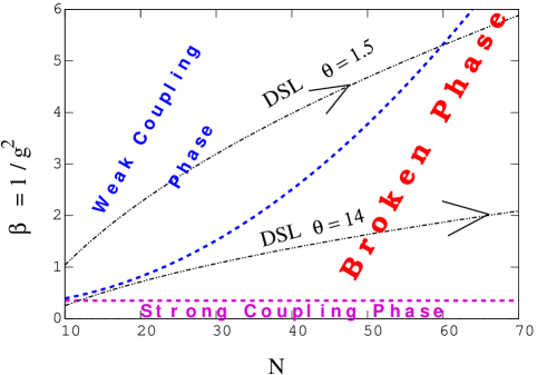
Figure 4. The phase diagram for QED₄ with a NC plane (in lattice units): between the strong coupling phase ($\beta\mathop{\raise 1.29167pt\hbox{$<$\kern-7.5pt\raise-4.73611pt\hbox{$\sim$}}}0.35$) and the weak coupling phase we recognise a phase of broken translation invariance. The weak/broken transition rises like $\beta\propto N^{2}$, whereas the DSL for a fixed NC parameter $\theta$ follows $\beta\propto\sqrt{N}$, so any DSL ends up in the broken phase.

The DSL is attained by following lines of constant $\theta$. Relation (12) implies that they correspond to $\beta\propto\sqrt{N}$, hence the DSL always leads to the broken phase. Since we found stability for a number of observables as we approach this limit, it seems to provide IR stability for the NC photon.

At last we consider non-perturbative results for the NC photon dispersion relation. The plot in Fig. 5 on the left shows the behaviour in the symmetric phase at weak coupling: it is fully consistent with the perturbative result of a negative IR divergence. However, we saw that the DSL leads to the broken phase, which is therefore physically relevant. For that phase the plot on the right of Fig. 5 reveals an IR stable behaviour, at least for the energy depending on the momentum component in the commutative space direction only, $E(p=p_{3})_{p_{1}=p_{2}=0}$.

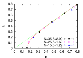
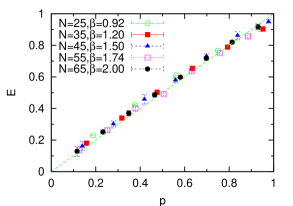
Figure 5. Dispersion relations $\,E(p)\$ for the photon in a NC space, in the weak coupling phase (on the left), and in the broken phase (on the right). The former result is consistent with the perturbatively predicted IR instability (“tachyonic” behaviour). In the physical phase, however, the photon is massless again, corresponding to a Nambu-Goldstone boson of the broken translation symmetry.

Therefore the photon could survive the transition to an NC world after all. Then one could again try to interpret it as the Nambu-Goldstone boson of the SSB of Poincaré symmetry, similar to the interpretation in the context of the SME [8] (cf. Section 1).

5. Conclusions

Cosmic $\gamma$-rays enable LI tests to extreme precision. So far LIV has not been detected anywhere — we reviewed failed attempts based on GRB data.

As theoretical frameworks leading to LIV we discussed on one side low energy effective theories [5, 6, 7, 8] and an effective ansatz which introduces particle specific Maximal Attainable Velocities [11]. Another approach is based on NC geometry — the presence of IR divergences in quantum field theory on such spaces clarifies its distinction from low energy effective theories.

In Section 4 we were concerned with the kinematics of a NC photon. Perturbation theory to one loop suggests its IR instability [39], which looks like a disaster for NC field theory. The picture changes, however, in light of a non-perturbative consideration.

Our numerical study revealed a phase of spontaneously broken Poincaré symmetry, which is not visible to perturbative calculations. In fact the limit to the continuum and to infinite volume at fixed non-commutativity (the Double Scaling Limit) leads to this phase of broken symmetry,and not to the symmetric weak coupling phase. In the broken symmetry phase we observed stability for a number of observables [41]. In particular the photon dispersion relation in a commutative sub-space appears linear. However, its behaviour at non-zero momentum components in the NC directions is not explored yet. In that respect, non-perturbative results could be confronted with phenomenological data — in particular from GRBs — to establish a robust bound on $\|\Theta\|$ in Nature. On the phenomenological side, more stringent data are expected from new large-scale GRB observations, for instance in the projects discussed in Refs. [28, 29].

Our non-perturbative results so far imply that the photon may survive in a NC world — despite the IR disaster on the 1-loop level — without the requirement to proceed to SUSY.

It was my pleasure to attend the 4^th EU RTN Workshop on “Constituents, Fundamental Forces and Symmetries of the Universe” in the beautiful city of Varna (Bulgaria), where this talk was presented. I would like to thank my collaborators for their contributions to Refs. [36, 40, 41, 34], the authors of Ref. [24] for their permission to reproduce Fig. 1, and F.W. Stecker for a helpful comment. This work was supported by the Deutsche Forschungsgemeinschaft (DFG) through Sonderforschungsbereich SFB/TR55 “Hadron Physics from Lattice QCD”.

References

- [1]
-
[2]
W. Pauli, Nuovo Cim. 6, 204 (1957).
G. Lüders, Ann. Phys. 2, 1 (1957).
R. Jost, Helv. Phys. Acta 30, 409 (1957). - [3] O.W. Greenberg, Phys. Rev. Lett. 89, 231602 (2002).
- [4] C. Amsler et al. (Particle Data Group), Phys. Lett. B 667, 1 (2008).
- [5] D. Colladay and V.A. Kostelecký, Phys. Rev. D 58, 116002 (1998).
- [6] R. Bluhm, Lect. Notes Phys. 702, 191 (2006).
-
[7]
D. Colladay and V.A. Kostelecký,
Phys. Rev. D 55, 6760 (1997).
V.A. Kostelecký and R. Lehnert, Phys. Rev. D 63, 065008 (2001). - [8] R. Bluhm and V.A. Kostelecký, Phys. Rev. D 71, 065008 (2005).
-
[9]
D. Mattingly,
Living Rev. Rel. 8, 5 (2005) 5; arXiv:0802.1561 [gr-qc].
V.A. Kostelecký and N. Russell, arXiv:0801.0287 [hep-ph]. - [10] J. Collins, A. Perez, D. Sudarsky, L. Urrutia and H. Vucetich, Phys. Rev. Lett. 93, 191301 (2004).
- [11] S.R. Coleman and S.L. Glashow, Phys. Rev. D 59, 116008 (1999).
-
[12]
R. Abbasi et al. (HiRes Collaboration),
Phys. Rev. Lett. 100, 101101 (2008).
J. Abraham et al. (Pierre Auger Collaboration), Phys. Rev. Lett. 101, 061101 (2008); arXiv:0906.2189 [astro-ph.HE]. -
[13]
S.T. Scully and F.W. Stecker,
arXiv:0811.2230 [astro-ph].
X.-J. Bi, Z. Cao, Y. Li and Q. Yuan, arXiv:0812.0121 [astro-ph]. - [14] W. Bietenholz, arXiv:0806.3713 [hep-ph].
- [15] G.L. Fogli, E. Lisi, A. Marrone and G. Scioscia, Phys. Rev. D 60, 053006 (1999). G. Battistoni et al., Phys. Lett. B 615, 14 (2005). M.C. Gonzalez-Garcia and M. Maltoni, Phys. Rev. D 70, 033010 (2004).
- [16] T. Jacobson, S. Liberati and D. Mattingly, Annals Phys. 321, 150 (2006).
- [17] T. Tanimori et al. (CANGAROO Collaboration), astro-ph/9710272.
- [18] F.A. Aharonian et al. (HEGRA Collaboration), Astron. Astrophys. 349, 11 (1999).
- [19] F. Krennrich et al., astro-ph/9808333.
- [20] P. Bhattacharjee and G. Sigl, Phys. Rept. 327, 109 (2000).
-
[21]
G. Amelino-Camelia and T. Piran,
Phys. Lett. B 497, 265 (2001); Phys. Rev. D 64, 036005 (2001).
R.J. Protheroe and H. Meyer, Phys. Lett. B 493, 1 (2000). - [22] F.W. Stecker and S.L. Glashow, Astropart. Phys. 16, 97 (2001). O.C. de Jager and F.W. Stecker, Astrophys. J. 566, 738 (2002).
- [23] G. Amelino-Camelia, J.R. Ellis, N.E. Mavromatos, D.V. Nanopoulos and S. Sarkar, Nature 393, 763 (1998).
- [24] J.R. Ellis, N.E. Mavromatos, D.V. Nanopoulos, A.S. Sakharov and E.K.G. Sarkisyan, Astropart. Phys. 25, 402 (2006); Erratum, arXiv:0712.2781 [astro-ph].
- [25] S.E. Boggs, C.B. Wunderer, K. Hurley and W. Coburn, Astrophys. J. 611, L77 (2004). M. Rodriguez Martinez and T. Piran, JCAP 0605, 017 (2006). J. Albert et al. (MAGIC Collaboration), and J.R. Ellis, N.E. Mavromatos, D.V. Nanopoulos, A.S. Sakharov and E.K.G. Sarkisyan, Phys. Lett. B 668, 253 (2008).
- [26] M.S. Brotherton, H.D. Tran, W. van Breugel, A. Dey and R. Antonucci, Astrophys. J. Lett. 487, L113 (1997).
- [27] R.J. Gleiser and C.N. Kozameh, Phys. Rev. D 64, 083007 (2001).
- [28] R. Lamon, JCAP 0808, 022 (2008) 022.
- [29] S. Basa, J. Wei, J. Paul and S.N. Zhang (for the SVOM Collaboration), arXiv:0811.1154 [astro-ph].
- [30] S. Doplicher, K. Fredenhagen and J.E. Roberts, Commun. Math. Phys. 172, 187 (1995).
- [31] R.J. Szabo, Phys. Rept. 378, 207 (2003).
- [32] A. González-Arroyo and M. Okawa, Phys. Rev. D 27, 2397 (1983).
-
[33]
H. Aoki, N. Ishibashi, S. Iso, H. Kawai,
Y. Kitazawa and T. Tada,
Nucl. Phys. B 565, 176 (2000).
J. Ambjørn, Y. Makeenko, J. Nishimura and R.J. Szabo, JHEP 11, 29 (1999); Phys. Lett. B 480, 399 (2000); JHEP 05, 023 (2000). - [34] W. Bietenholz, F. Hofheinz and J. Nishimura, JHEP 0209, 009 (2002).
- [35] N. Seiberg and E. Witten, JHEP 9909, 032 (1999).
- [36] W. Bietenholz, A. Bigarini and A. Torrielli, JHEP 0708, 041 (2007).
- [37] A. Matusis, L. Susskind and N. Toumbas, JHEP 0012, 002 (2000).
- [38] G. Amelino-Camelia, L. Doplicher, S.-K. Nam and Y.-S. Seo, Phys. Rev. D 67, 085008 (2003).
- [39] F. Ruiz Ruiz, Phys. Lett. B 502, 274 (2001). K. Landsteiner, E. Lopez and M.H.G. Tytgat, JHEP 0106, 055 (2001). M. Van Raamsdonk, JHEP 0111, 006 (2001).
- [40] W. Bietenholz, F. Hofheinz and J. Nishimura, JHEP 0406, 042 (2004).
- [41] W. Bietenholz, J. Nishimura, Y. Susaki and J. Volkholz, JHEP 0610, 042 (2006).
-
[42]
M. Teper and H. Vairinhos,
Phys. Lett. B 652, 359 (2007).
T. Azeyanagi, M. Hanada, T. Hirata and T. Ishikawa, JHEP 0801, 025 (2008).