Oscillations of Rapidly Rotating Superfluid Stars

Abstract

Using time evolutions of the relevant linearised equations we study non-axisymmetric oscillations of rapidly rotating and superfluid neutron stars. We consider perturbations of Newtonian axisymmetric background configurations and account for the presence of superfluid components via the standard two-fluid model. Within the Cowling approximation, we are able to carry out evolutions for uniformly rotating stars up to the mass-shedding limit. This leads to the first detailed analysis of superfluid neutron star oscillations in the fast rotation regime, where the star is significantly deformed by the centrifugal force. For simplicity, we focus on background models where the two fluids (superfluid neutrons and protons) co-rotate, are in $\beta$-equilibrium and coexist throughout the volume of the star. We construct sequences of rotating stars for two analytical model equations of state. These models represent relatively simple generalisations of single fluid, polytropic stars. We study the effects of entrainment, rotation and symmetry energy on non-radial oscillations of these models. Our results show that entrainment and symmetry energy can have a significant effect on the rotational splitting of non-axisymmetric modes. In particular, the symmetry energy modifies the inertial mode frequencies considerably in the regime of fast rotation.

1 Introduction

According to the standard paradigm, millisecond pulsars are accelerated to their fast rotation rates by accreting matter from a close companion. This means that they tend to be relatively old. Moreover, the fastest spinning pulsars should have weak (exterior) magnetic fields. In the standard accretion model, neutron stars with canonical $10^{12}$ G dipole fields will reach equilibrium already at a modest spin. A weak surface field is also expected since accretion leads to magnetic field burial. This picture agrees well with observational data. Rapidly rotating neutron stars are most commonly found in binary systems. It is well established that accreting neutron stars in low-mass X-ray binaries (where the angular momentum transfer is more efficient due to the long evolution time of the low mass partner) can reach a millisecond rotation period. Furthermore, the fastest known millisecond pulsar J1748-2446ad, with a period of 1.39 ms (Hessels et al., 2006), is in a binary system. In fact, its companion, with mass $M\geq 0.14M_{\odot}$, could still fill the Roche lobe powering the spin-up phase further. The mass and radius of J1748-2446ad are unknown, but combining reasonable ranges for these parameters, $M=1.4-2M_{\odot}$ and $R=10-14~{}\rm{km}$, with an empirical formula for the maximum rotation of the star (Lattimer & Prakash, 2004)

$$\Omega_{K}\approx 6566\left(\frac{M}{M_{\odot}}\right)^{1/2}\left(\frac{10\rm{km}}{R}\right)^{3/2}\rm{Hz}\,,$$ (1)

one finds that the spin of this object lies in the range $0.48\mathrel{\hbox{\hbox to0.0pt{\hbox{\lower 4.0pt\hbox{$\sim$}}\hss}\hbox{$<$}}}\Omega/\Omega_{K}\mathrel{\hbox{\hbox to0.0pt{\hbox{\lower 4.0pt\hbox{$\sim$}}\hss}\hbox{$<$}}}0.96$. In other words, it could be close to the mass-shedding limit.

The temperature of a mature neutron star is likely below the critical temperature, $T_{c}\simeq 5\times 10^{9}$ K, where neutrons and protons are superfluid and superconducting, respectively. Depending on the cooling mechanism, neutrino emission can cool a hot proto-neutron star below this temperature shortly after its formation in a core collapse supernova (see e.g, Page, Geppert & Weber, 2006). In an accreting system, the neutron star core temperature is not expected to increase beyond $T_{c}$ (nuclear burning in the accreted surface layers is thought to the heat the core to $\sim 10^{8}$ K). Hence, all mature neutron stars should contain degenerate superfluid neutrons in the outer core and the inner crust and degenerate superconducting protons in the outer core. The deep core may contain more exotic phases of matter, like superfluid hyperons and/or colour superconducting quarks. Superfluidity influences the thermal evolution and the dynamical properties of a neutron star. In particular, the dynamics is strongly affected by entrainment, the formation of quantized neutron vortices, and the presence of new dissipative mechanisms like mutual friction. An understanding of superfluid dynamics is crucial for modelling many aspects of the neutron star physics, ranging from pulsar glitches and free precession to the mutual friction damping of stellar oscillations and associated instabilities.

Tidal forces, accretion and glitches may trigger oscillations and/or instabilities in rapidly rotating neutron stars. Observations of such oscillations, either via electromagnetic or gravitational radiation, would help us explore the exotic physics of these compact objects (Andersson & Kokkotas, 1998; Benhar et al., 2004; Samuelsson & Andersson, 2007). In this context it is interesting to note the differences in dynamics between neutron stars above the superfluid transition temperature and colder systems. The core of a hot young neutron star is relatively well described by the Navier-Stokes equations. In contrast, a star with a superfluid core requires a multi-fluid description. The standard model for such systems is inspired by the two-fluid model for superfluid Helium (Landau & Lifshitz, 1959; Khalatnikov, 1965; Tilley & Tilley, 1990). The oscillation spectrum of superfluid neutron stars reflects the presence of the additional degree of freedom (Epstein, 1988). Basically, the perturbed fluid elements in a two-fluid system can oscillate either in phase or in a counter-phase motion. Previous studies, see for example, Lee (1995); Andersson & Comer (2001); Prix & Rieutord (2002); Yoshida & Lee (2003a), have established that co-moving pulsations have spectral properties similar to single fluid stars. Hence, it is natural to refer to such modes as “ordinary” modes. The counter-moving degree of freedom leads to new oscillation modes that are specific to the two-fluid systems. These are often referred to as “superfluid” modes. Later, when we write down the perturbation equations for a superfluid neutron star core, we choose to work with variables that are directly associated with the two types of motion. This is natural if we want to distinguish spectral properties associated with the “superfluid” degree of freedom. In addition, we use the standard classification of neutron star oscillation modes, based on the main restoring force that acts on a perturbed fluid element. A rotating single fluid star can sustain acoustic and inertial modes restored by pressure and the Coriolis force, respectively. When thermal or composition gradients are present in the star, buoyancy acts as restoring force for the so-called gravity modes (Unno et al., 1989; Reisenegger & Goldreich, 1992). Previous work has shown that superfluid neutron stars have two families of acoustic and inertial modes, more or less clearly (depending on the stellar model) associated with the co- and counter-moving fluid motion. It is, however, not the case that all single fluid modes have a ”double” in the superfluid problem. The gravity modes are not present at all in a superfluid core (Lee, 1995; Andersson & Comer, 2001; Prix & Rieutord, 2002). Their absence provides a potentially important signature for neutron star seismology.

Rapidly rotating neutron stars have been studied in detail with a variety of methods (see e.g., Stergioulas, 2003). Yet, there have not been any previous studies of multi-fluid dynamics in the rapid rotation regime near the break-up limit. The oscillation modes of superfluid neutron stars have only been calculated in the frequency domain using the slow rotation approximation (Lindblom & Mendell, 2000; Yoshida & Lee, 2003a, b). In that framework, the effects of the stellar rotation are determined perturbatively as corrections to the non-rotating results. The only previous attempt (that we are aware of) to study superfluid oscillations for truly fast spinning stars is the work by Lindblom & Mendell (2000). They extended the two-potential formalism of Ipser & Lindblom (1990) to the superfluid case. However, due to numerical difficulties they could not study rotating models near the break-up limit. Neither did they manage to determine the superfluid modes.

In this work, we study the time evolution of perturbed fast rotating, Newtonian superfluid neutron stars within the Cowling approximation. As far as we are aware, this is the first study that evolves in time the oscillations of superfluid neutron stars. Moreover, it is the first detailed analysis of the rapid rotation regime. Within the framework of the two-fluid formalism, we carry out a linear perturbation analysis for stationary and axisymmetric equilibrium configurations. As preparation for more detailed studies, we consider relatively simple models where the two fluids coexist throughout the star, and where the unperturbed configuration is in $\beta$-equilibrium. These assumptions imply that the two fluids are co-rotating and share the same external stellar surface in our background configurations. We use these models to investigate the effects of entrainment, symmetry energy and rotation on the superfluid oscillation spectrum. In order to establish the reliability of our numerical evolution code, we compare our results to previous work for non-rotating and slowly rotating models. We then consider, for the first time, the dynamics of superfluid models rotating up to the mass shedding limit.

2 Equations of Motion

We use the two-fluid framework for superfluid neutron stars (Mendell, 1991a, b; Prix, 2004; Andersson & Comer, 2006). This model distinguishes between a superfluid neutron component and a neutral mixture of protons and electrons. The charged particles are assumed to be locked together by the electromagnetic interaction on a timescale much shorter than the dynamics we consider. For simplicity, we refer to the charged particle conglomerate as the “protons” from now on. When the mass of each component is conserved the dynamics is described by two mass conservation laws, two Euler-type equations and the Poisson equation for the gravitational potential (Prix, 2004):

$$\partial_{t}\rho_{\mathrm{x}}+\nabla_{i}\left(\rho_{\mathrm{x}}v_{\mathrm{x}}^{i}\right)=0\,,\\$$ (2)

$$\left(\partial_{t}+v_{\mathrm{x}}^{k}\nabla_{k}\right)\left(v_{i}^{\mathrm{x}}+\varepsilon_{\mathrm{x}}w_{i}^{\mathrm{y}\mathrm{x}}\right)+\nabla_{i}\left(\Phi+\tilde{\mu}_{\mathrm{x}}\right)+\varepsilon_{\mathrm{x}}w_{k}^{\mathrm{y}\mathrm{x}}\nabla_{i}v_{\mathrm{x}}^{k}=\frac{f^{\mathrm{x}}_{i}}{\rho_{\mathrm{x}}}\,,\\$$ (3)

$$\nabla^{2}\Phi=4\pi G\rho\,.$$ (4)

Here the indices $i$ and $k$ label the spatial components of the vectors while $\mathrm{x}$ and $\mathrm{y}$ denote the two fluid components. The constituent indices take the values $\mathrm{n}$ for the neutrons and $\mathrm{p}$ for the protons. Note that the summation rule for repeated indices applies only for spatial and not for constituent indices. In equations (2)–(4), $\rho=\rho_{\mathrm{n}}+\rho_{\mathrm{p}}$ and $\Phi$ represent the total mass density and the gravitational potential, respectively. Meanwhile, $\mathbf{f}^{\mathrm{x}}$ is the force density acting on the $\mathrm{x}$ fluid component. In this work, we consider an isolated system where dissipation processes, like mutual friction, are absent. We then have $\mathbf{f}^{\mathrm{x}}=\mathbf{0}$. Furthermore, we have assumed that the particle masses are equal, $m=m_{\mathrm{n}}=m_{\mathrm{p}}$, and defined the chemical potential and the relative velocity between the two fluids as follows:

$$\tilde{\mu}_{\mathrm{x}} \equiv \left.\frac{\partial\mathcal{E}}{\partial\rho_{\mathrm{x}}}\right|_{\rho_{\mathrm{y}},w_{\mathrm{x}\mathrm{y}}^{2}}\,,$$ (5)

$$w^{\mathrm{x}\mathrm{y}}_{i} \equiv v_{i}^{\mathrm{x}}-v_{i}^{\mathrm{y}}\,.$$ (6)

The energy functional $\mathcal{E}=\mathcal{E}(n_{\mathrm{n}},n_{\mathrm{p}},w_{\mathrm{n}\mathrm{p}}^{2})$ describes the equation of state (EoS) of the system. Finally, the non-dissipative entrainment between the two fluids is governed by the parameter $\varepsilon_{\mathrm{x}}$, which follows from the definition:

$$\varepsilon_{\mathrm{x}}\equiv 2\rho_{\mathrm{x}}\left.\frac{\partial\mathcal{E}}{\partial w^{2}_{\mathrm{n}\mathrm{p}}}\right|_{\rho_{\mathrm{x}},\rho_{\mathrm{y}}}\,.$$ (7)

The equations that describe rapidly and uniformly rotating background models can be derived by integrating the Euler-type equations (3) and the Poisson equation (4) (Prix et al., 2002; Yoshida & Eriguchi, 2004). This leads to

$$\tilde{\mu}_{\mathrm{x}}+\Phi-\frac{r^{2}}{2}\sin\theta^{2}\,\Omega_{\mathrm{x}}^{2}=C_{\mathrm{x}}\,,$$ (8)

where $\Omega_{\mathrm{x}}$ and $C_{\mathrm{x}}$ are, respectively, the angular velocities and the integration constants for the neutron and proton fluids. In this work, we focus on corotating background models, $\Omega_{\mathrm{n}}=\Omega_{\mathrm{p}}=\Omega$, where the two fluids are in $\beta$-equilibrium and have a common surface. The hydrostatic equilibrium equation (8) then become

$$\tilde{\mu}+\Phi-\frac{r^{2}}{2}\sin\theta^{2}\,\Omega^{2}=C\,,$$ (9)

where $\tilde{\mu}_{\mathrm{p}}=\tilde{\mu}_{\mathrm{n}}\equiv\tilde{\mu}$ is the background chemical potential and $C\equiv C_{\mathrm{n}}=C_{\mathrm{p}}$. It is worth noticing that equations (4) and (9) are formally equivalent to the single fluid problem provided one replaces the chemical potential with the enthalpy (Yoshida & Eriguchi, 2004). Given an equation of state, equations (4) and (9) can be numerically solved using the self-consistent field method of Hachisu (1986). The surface of the star corresponds to the zero chemical potential surface, $\tilde{\mu}\left(r\left(\theta\right),\theta\right)=0$ (Yoshida & Eriguchi, 2004).

3 Perturbation Equations

It is straighforward to write down the system of partial differential equations that governs the Eulerian perturbations $\delta\rho_{\mathrm{x}},\delta\mathbf{v}_{\mathrm{x}},\delta\tilde{\mu}_{\mathrm{x}}$ and $\delta\Phi$. However, instead of working with these variables, we define (see Andersson, Glampedakis & Haskell, 2008, for a detailed discussion) new variables which are more closely related to the natural degrees of freedom of the problem. In the rotating frame, the co-moving (ordinary) motion is described by the mass flux $\mathbf{f}$ (not to be confused with the mutual force $\mathbf{f}^{\mathrm{x}}$), the total mass density $\delta\rho$ and the pressure $\delta P$, defined by

$$\mathbf{f} = \rho_{\mathrm{p}}\mathbf{v}_{\mathrm{p}}+\rho_{\mathrm{n}}\mathbf{v}_{\mathrm{n}}\,,$$ (10)

$$\delta\rho = \delta\rho_{\mathrm{n}}+\delta\rho_{\mathrm{p}}\,,$$ (11)

$$\nabla\delta P = \rho_{\mathrm{p}}\nabla\delta\tilde{\mu}_{\mathrm{p}}+\rho_{\mathrm{n}}\nabla\delta\tilde{\mu}_{\mathrm{n}}\,.$$ (12)

Meanwhile, the counter-moving (superfluid) motion is described by a vector field $\mathbf{D}$ that is proportional to the relative velocity between the two fluids, the scalar perturbation $\delta\beta$ that measures the deviation from $\beta$-equilibrium and the quantity $\delta\chi_{\mathrm{p}}$, which is related to the perturbed proton fraction. These variables are defined by

$$\mathbf{D} = x_{\mathrm{p}}\left(1-x_{\mathrm{p}}\right)\rho\left(\mathbf{v}_{\mathrm{p}}-\mathbf{v}_{\mathrm{n}}\right)\,,$$ (13)

$$\delta\beta = \delta\tilde{\mu}_{\mathrm{p}}-\delta\tilde{\mu}_{\mathrm{n}}\,,$$ (14)

$$\delta\chi_{\mathrm{p}} = \rho\,\delta x_{\mathrm{p}}\,,$$ (15)

where $x_{\mathrm{p}}=\rho_{\mathrm{p}}/\rho$ is the proton fraction.

In order to simplify the evolutions, we neglect the perturbations of the gravitational potential $\delta\Phi=0$. That is, we adopt the Cowling approximation. This approximation should be quite accurate for inertial modes. For low order acoustic modes, like the f-mode, it is not so accurate but the results are still qualitatively correct. For our present purposes, this should be sufficent. Although, it would not be too difficult to solve also for the perturbed gravitational potential it is computationally costly to add the solution of an elliptic equation to our evolutions. Hence, we decided not to solve the full problem in this first exploratory study.

In the frame of the rotating background the final perturbation equations can be written

$$\partial_{t}\mathbf{f} = -\nabla\delta P-2\mathbf{\Omega}\times\mathbf{f}+\frac{\nabla P}{\rho}\,\delta\rho\,,$$ (16)

$$\partial_{t}\mathbf{D} = -\frac{x_{\mathrm{p}}\left(1-x_{\mathrm{p}}\right)\rho\nabla\delta\beta}{1-\bar{\varepsilon}}-\frac{2\mathbf{\Omega}\times\mathbf{D}}{1-\bar{\varepsilon}}\,,$$ (17)

$$\partial_{t}\delta\rho = -\nabla\cdot\mathbf{f}\,,$$ (18)

$$\partial_{t}\delta\chi_{\mathrm{p}} = -\nabla\cdot\mathbf{D}-\mathbf{f}\cdot\nabla x_{\mathrm{p}}\,,$$ (19)

where we have defined $\bar{\varepsilon}=\varepsilon_{\mathrm{n}}/x_{\mathrm{p}}$.

The time evolution of the non-axisymmetric perturbation equations is a three-dimensional problem in space. However, linear perturbations on an axisymmetric background can be expanded in terms of a set of basis functions $\left(\cos m\phi\,,\sin m\phi\right)$, where $m$ is the azimuthal harmonic index (Papaloizou & Pringle, 1980). The mass density perturbations as well as the other perturbation quantities take the following form (Jones et al., 2002; Passamonti et al., 2009)

$$\delta\rho\left(t,r,\theta,\phi\right)=\sum_{m=0}^{m=\infty}\left[\delta\rho_{m}^{+}\left(t,r,\theta\right)\cos m\phi+\delta\rho_{m}^{-}\left(t,r,\theta\right)\sin m\phi\right]\,.$$ (20)

The perturbation equations now decouple with respect to $m$ and the problem becomes two-dimensional. Therefore for any $m$, the non-axisymmetric oscillations of a superfluid neutron star requires the solution of a system of eighteen partial differential equations for the twenty variables $\left(\mathbf{f}^{\pm},\delta\rho^{\pm},\delta P^{\pm},\mathbf{D}^{\pm},\delta\chi_{\mathrm{p}}^{\pm},\delta\beta^{\pm}\right)$. To fully specify the problem, the set of equations (16)-(19) must be complemented by two relations that depend on the EoS (see Section 4).

3.1 Boundary Conditions

In order to evolve the perturbation equations we must also specify boundary conditions. For non-axisymmetric oscillations with $m\geq 2$, equations (16)–(19) are regular at the origin, $r=0$, when the following conditions are satisfied:

$$\delta P=\delta\chi_{\mathrm{p}}=\delta\beta=\delta\rho=0\,,\qquad\textrm{and}\qquad\mathbf{f}=\mathbf{D}=\mathbf{0}\,.$$ (21)

For the boundary condition at the stellar surface, it is worth remembering that the unperturbed configuration is such that the two fluids have a common surface (see Section 1). At the perturbed level, we require that the Lagrangian perturbation of the chemical potentials vanishes at the surface, i.e.,

$$\Delta_{\mathrm{x}}\tilde{\mu}_{\mathrm{x}}=\delta\tilde{\mu}_{\mathrm{x}}+\mathbf{\xi}_{\mathrm{x}}\cdot\nabla\tilde{\mu}_{\mathrm{x}}=0\,,$$ (22)

where the Lagrangian variations $\Delta_{\mathrm{x}}$ are associated with the fluid displacements $\mathbf{\xi}_{\mathrm{x}}$ (Andersson, Comer & Grosart, 2004). Equations (22) can be expressed in terms of $\delta P$ and $\delta\beta$ by using the definitions (12) and (14). This leads to

$$\Delta P = \delta P+\left[x_{\mathrm{p}}\,\mathbf{\xi}_{\mathrm{p}}+\left(1-x_{\mathrm{p}}\right)\mathbf{\xi}_{\mathrm{n}}\right]\cdot\nabla P=0\,,$$ (23)

$$\Delta\beta = \delta\beta+\left(\mathbf{\xi}_{\mathrm{p}}-\mathbf{\xi}_{\mathrm{n}}\right)\cdot\frac{\nabla P}{\rho}=0\,,$$ (24)

where we have used the fact that the background model is in $\beta$-equilibrium condition, i.e., $\tilde{\mu}_{\mathrm{n}}=\tilde{\mu}_{\mathrm{p}}$. As in the single fluid case we can derive a simpler condition for the pressure perturbation. From the Euler equation for the stationary background (noting that (12) holds also at the unperturbed level)

$$\nabla P=-\rho\mathbf{\Omega}\times\left(\mathbf{\Omega}\times\mathbf{r}\right)-\rho\nabla\Phi\,,$$ (25)

and the fact that the EoS used in this work are such that the total mass density vanishes at the surface, it follows that equation (23) is equivalent to (Tassoul, 1978):

$$\delta P=0\,.$$ (26)

This condition is numerically convenient, and ensures that all variables remain regular at the surface.

The reflection symmetry with respect to the equator divides the perturbation variables into two sets (Passamonti et al., 2009). Perturbations of the Type I parity class have $\left(f_{r},f_{\phi},\delta\rho,\delta P,D_{r},D_{\phi},\delta\chi_{\mathrm{p}},\delta\beta\right)$ even and $\left(f_{\theta},D_{\theta}\right)$ odd. The opposite is true for perturbations of Type II.

4 Equation of State

To complete the formulation of the superfluid oscillation problem we need to supply a suitable multi-parameter equation of state. In a truly realistic model, the equation of state should be obtained from a microscopic (quantum) analysis. It will completely specify not only the relation between pressure and density, but also the composition and the detailed superfluid energy gaps for neutrons and protons. Moreover, it has to also provide the entrainment parameters. We do not yet have such a model, although recent developments in this direction are promising (Chamel, 2008). Given this, and the fact that our main aim is to understand the oscillations of a rotating superfluid neutron star at the qualitative level, we will opt to work with two simple analytic model equations of state. These models, described in Sections 5.1 and  5.2 below, are natural generalisations of the single fluid polytropes. The analytical models are particularly useful since they allow us to tune key parameters like entrainment and symmetry energy more or less freely. As we will see, we can also vary the coupling between the co- and counter-moving fluid degrees of freedom.

Quite generally, the required energy functional can be expressed as a function of the two fluid mass densities and the relative velocity:

$$\mathcal{E}=\mathcal{E}\left(\rho_{\mathrm{n}},\rho_{\mathrm{p}},w_{\mathrm{n}\mathrm{p}}^{2}\right)\,,$$ (27)

where the dependence on $\mathbf{w}_{\mathrm{n}\mathrm{p}}$ ensures Galilean invariance. For a small relative velocity between the two fluids, equation (27) can be written

$$\mathcal{E}=\mathcal{E}_{0}\left(\rho_{\mathrm{n}},\rho_{\mathrm{p}}\right)+\alpha_{0}\left(\rho_{\mathrm{n}},\rho_{\mathrm{p}}\right)w_{\mathrm{n}\mathrm{p}}^{2}+\mathcal{O}\left(w_{\mathrm{n}\mathrm{p}}^{4}\right)\,,$$ (28)

in which case the bulk EoS $\mathcal{E}_{0}$ and the entrainment $\alpha_{0}$ can be independently specified at $\mathbf{w}_{\mathrm{n}\mathrm{p}}=\mathbf{0}$. From equation (7) follows that the entrainment parameter $\varepsilon_{\mathrm{x}}$ is related to the function $\alpha_{0}$ by

$$\rho_{\mathrm{x}}\varepsilon_{\mathrm{x}}=2\alpha_{0}\,.$$ (29)

Having specified the EoS, we must determine two equations that close the system (16)–(19). One possible choice is to determine the pressure perturbation and the quantity $\delta\beta$ from the total density and the proton fraction

$$\delta P=\delta P\left(\delta\rho,\delta x_{\mathrm{p}}\right)\,,\qquad\qquad\delta\beta=\delta\beta\left(\delta\rho,\delta x_{\mathrm{p}}\right)\,.$$ (30)

The required relations are obtained by first expressing these quantities in terms of the chemical potential perturbations $\delta\tilde{\mu}_{\mathrm{x}}$, i.e. using the thermodynamic definitions

$$\delta P = \rho_{\mathrm{p}}\delta\tilde{\mu}_{\mathrm{p}}+\rho_{\mathrm{n}}\delta\tilde{\mu}_{\mathrm{n}}\,,$$ (31)

$$\delta\beta = \delta\tilde{\mu}_{\mathrm{p}}-\delta\tilde{\mu}_{\mathrm{n}}\,.$$ (32)

For corotating background models ($\mathbf{w}_{\mathrm{n}\mathrm{p}}=\mathbf{0}$), the perturbation of the chemical potential $\tilde{\mu}_{\mathrm{x}}=\tilde{\mu}_{\mathrm{x}}\left(\rho_{\mathrm{p}},\rho_{\mathrm{n}}\right)$ can be expressed as

$$\delta\tilde{\mu}_{\mathrm{x}}=\left.\frac{\partial\tilde{\mu}_{\mathrm{x}}}{\partial\rho_{\mathrm{p}}}\right|_{\rho_{\mathrm{n}}}\delta\rho_{\mathrm{p}}+\left.\frac{\partial\tilde{\mu}_{\mathrm{x}}}{\partial\rho_{\mathrm{n}}}\right|_{\rho_{\mathrm{p}}}\delta\rho_{\mathrm{n}}\,,$$ (33)

where the mass densities of the two fluid components are defined in terms of the total mass density and proton fraction by

$$\delta\rho_{\mathrm{p}} = x_{\mathrm{p}}\delta\rho+\rho\,\delta x_{\mathrm{p}}\,,$$ (34)

$$\delta\rho_{\mathrm{n}} = \left(1-x_{\mathrm{p}}\right)\delta\rho-\rho\,\delta x_{\mathrm{p}}\,.$$ (35)

By introducing equations (33)–(35) into equations (31)–(32), we obtain:

$$\delta P = \left[\left(\left(1+2\sigma\right)x_{\mathrm{p}}^{2}-2\left(1+\sigma\right)x_{\mathrm{p}}+1\right)A_{\mathrm{n}\mathrm{n}}+x_{\mathrm{p}}^{2}A_{\mathrm{p}\mathrm{p}}\right]\rho\,\delta\rho+\left[\left(\left(1+2\sigma\right)x_{\mathrm{p}}-1-\sigma\right)A_{\mathrm{n}\mathrm{n}}+x_{\mathrm{p}}A_{\mathrm{p}\mathrm{p}}\right]\rho\,\delta\chi_{\mathrm{p}}\,,$$ (36)

$$\delta\beta = \left[\left(\left(1+2\sigma\right)x_{\mathrm{p}}-1-\sigma\right)A_{\mathrm{n}\mathrm{n}}+x_{\mathrm{p}}A_{\mathrm{p}\mathrm{p}}\right]\delta\rho+\left[\left(1+2\sigma\right)A_{\mathrm{n}\mathrm{n}}+A_{\mathrm{p}\mathrm{p}}\right]\delta\chi_{\mathrm{p}}\,,$$ (37)

where the matrix $A_{\mathrm{x}\mathrm{y}}$ is defined by

$$A_{\mathrm{x}\mathrm{y}}\equiv\frac{\partial\tilde{\mu}_{\mathrm{x}}}{\partial\rho_{\mathrm{y}}}=\frac{\partial^{2}\mathcal{E}}{\partial\rho_{\mathrm{y}}\partial\rho_{\mathrm{x}}}\,,$$ (38)

and $\sigma$ corresponds to the so-called “symmetry energy” (Prix, Comer & Andersson, 2002; Prakash, Lattimer & Ainsworth, 1988). That is, we have

$$\sigma\equiv-\frac{A_{\mathrm{n}\mathrm{p}}}{A_{\mathrm{n}\mathrm{n}}}\,.$$ (39)

5 Stellar Models

Background stellar models such that the two fluids are co-rotating can be constructed by solving the hydrostatic equilibrium equations (4) and (9) for a given bulk EoS $\mathcal{E}_{0}$, cf.  (28). Since equations (4) and (9) are formally equivalent to the equilibrium equations for a single fluid polytrope, we can straightforwardly use the method of Hachisu (1986) to determine such background models (see Section 2).

For a co-rotating background, entrainment does not not affect the equilibrium configuration. Hence, it can be chosen independently from the bulk EoS (see equations (28) and (29)). In fact, the entrainment parameter appears only in the perturbation equation (17) through the combination

$$\bar{\varepsilon}=\frac{\varepsilon_{\mathrm{n}}}{x_{\mathrm{p}}}=\varepsilon_{\mathrm{p}}+\varepsilon_{\mathrm{n}}\,.$$ (40)

In the last step we have used the relation (29), i.e. $\rho_{\mathrm{n}}\varepsilon_{\mathrm{n}}=\rho_{\mathrm{p}}\varepsilon_{\mathrm{p}}$. Nuclear physics calculations limit the value of the entrainment in the neutron star core to $0.2\leq\varepsilon_{\mathrm{p}}\leq 0.8$, see Chamel (2008) for a recent analysis. However, values outside this range are possible, especially for the crust superfluid. In fact, the parameter $\varepsilon_{\mathrm{p}}$ is expected to have negative values in the crust region (Chamel, 2006). Since we are interested in exploring the effect that the different parameters have on the neutron star oscillation modes, we will consider the range $-0.7\leq\bar{\varepsilon}\leq 0.7$.

5.1 Model A

Table 1: This table provides the main parameters for the rotating models A and B (see Sections 5.1 and 5.2 for the detailed EoS). The first column labels each model. In the second and third columns we show, respectively, the ratio of polar to equatorial axes and the angular velocity of the star. In the fourth column, the rotation rate is compared to the Kepler velocity $\Omega_{K}$ that represents the mass shedding limit. The ratio between the rotational kinetic energy and gravitational potential energy $T/|W|$ and the stellar mass are given in the fifth and sixth columns, respectively. All quantities are given in dimensionless units, where $G$ is the gravitational constant, $\rho_{c}$ represents the central mass density and $R_{eq}$ is the equatorial radius.

Model	$R_{p}/R_{eq}$	$\Omega/\sqrt{G\rho_{c}}$	$\Omega/\Omega_{K}$	$T/|W|\times 10^{2}$	$M/(\rho_{c}R_{eq}^{3})$
A0	1.000	0.000	0.000	0.000	1.273
A1	0.996	0.084	0.116	0.096	1.270
A2	0.983	0.167	0.230	0.385	1.248
A3	0.950	0.287	0.396	1.169	1.197
A4	0.900	0.403	0.556	2.385	1.118
A5	0.850	0.488	0.673	3.639	1.038
A6	0.800	0.556	0.767	4.933	0.956
A7	0.750	0.612	0.844	6.252	0.869
A8	0.700	0.658	0.907	7.568	0.779
A9	0.650	0.693	0.956	8.822	0.684
A10	0.600	0.717	0.989	9.865	0.579
A11	0.558	0.725	0.999	10.277	0.480
B0	1.000	0.000	0.000	0.000	1.833
B1	0.996	0.094	0.107	0.105	1.825
B2	0.983	0.187	0.213	0.419	1.799
B3	0.950	0.323	0.368	1.275	1.733
B4	0.900	0.453	0.516	2.608	1.632
B5	0.850	0.551	0.628	4.002	1.529
B6	0.800	0.629	0.717	5.459	1.424
B7	0.750	0.695	0.792	6.981	1.317
B8	0.700	0.751	0.856	8.566	1.207
B9	0.650	0.798	0.909	11.020	1.093
B10	0.600	0.835	0.952	11.862	0.973
B11	0.563	0.857	0.977	13.074	0.875
B12	0.496	0.877	0.999	14.613	0.669

As our first model equation of state we consider  (see, Prix et al., 2002; Yoshida & Eriguchi, 2004)

$$\mathcal{E}_{0}=\frac{1}{2}\sum_{\mathrm{x},\mathrm{y}}A_{\mathrm{x}\mathrm{y}}\rho_{\mathrm{x}}\rho_{\mathrm{y}}\,.$$ (41)

We will refer to this as model A. Despite its obvious simplicity, this model allows us to investigate the effect of the symmetry energy on the oscillation spectrum. This is apparent from the matrix coefficients $A_{\mathrm{x}\mathrm{y}}$ which have the following form:

$$A_{\mathrm{n}\mathrm{n}} = \frac{2K}{1-\left(1+\sigma\right)x_{\mathrm{p}}}\ ,$$ (42)

$$A_{\mathrm{p}\mathrm{p}} = \frac{2K\left[1+\sigma-\left(1+2\sigma\right)x_{\mathrm{p}}\right]}{x_{\mathrm{p}}\left[1-\left(1+\sigma\right)x_{\mathrm{p}}\right]}\,,$$ (43)

$$\qquad A_{\mathrm{n}\mathrm{p}} = -\sigma A_{\mathrm{n}\mathrm{n}}\,,$$ (44)

where $\sigma$ and $K$ are constants. Equations (42)–(44) are equivalent to the set used by Yoshida & Eriguchi (2004) with $2K=1/k$. From the $\beta$-equilibrium condition for the stellar background, $\tilde{\mu}_{\mathrm{n}}=\tilde{\mu}_{\mathrm{p}}$, and the definition (5) we can derive the proton fraction for these models

$$x_{\mathrm{p}}=\frac{\left(1+\sigma\right)A_{\mathrm{n}\mathrm{n}}}{A_{\mathrm{p}\mathrm{p}}+\left(1+2\sigma\right)A_{\mathrm{n}\mathrm{n}}}\,.$$ (45)

If we take the coefficients $A_{\mathrm{x}\mathrm{y}}$ to be constant, model A leads to a family of non-stratified stars. The perturbation variables are related by equations (36)–(37) which in this case become

$$\delta P=2K\rho\,\delta\rho\,,\qquad\qquad\delta\beta=\frac{2K\left(1+\sigma\right)}{x_{\mathrm{p}}\left[1-\left(1+\sigma\right)x_{\mathrm{p}}\right]}\delta\chi_{\mathrm{p}}\,.$$ (46)

Therefore, the models are specified by the three parameters $K,\sigma$ and $x_{\mathrm{p}}$. For this class of models, the degrees of freedom that describe the co- and counter-moving fluid motion are decoupled. The variables $\mathbf{f},\delta\rho,\delta P$ evolve independently from $\mathbf{D},\delta\chi_{\mathrm{p}},\delta\beta$. This is a useful simplification that helps the interpretation of the oscillation spectrum.

For a background star in $\beta$-equilibrium, the chemical potential is related to the total mass density by

$$\tilde{\mu}=2K\rho\,,$$ (47)

which means that the pressure is that of the usual $N=1$ polytrope:

$$P=K\rho^{2}\,.$$ (48)

We have constructed a family of rotating stars for this equation of state. In dimensionless units, the constant $K$ is determined automatically by specifying the polytropic index and the axis ratio between the polar and equatorial radius $R_{p}/R_{eq}$ (Jones et al., 2002; Passamonti et al., 2009). The properties of our rotating models are given in Table 1, where we also label each member of the sequence. The non-rotating model is refered to as A0 and the fastest rotating model is A11. Being non-stratified stars, the values of both the proton fraction $x_{\mathrm{p}}$ and the symmetry energy term $\sigma$ affect only the counter-moving motion of the perturbed fluid. In fact, they appear only in the perturbation equations (17) and (19), and in equation (46) for the $\delta\beta$ perturbation. In our numerical simulations, we focus mainly on stars with $x_{\mathrm{p}}=0.1$ and $-1\leq\sigma\leq 1$. The range of the symmetry energy is constrained by the requirement that $A_{\mathrm{x}\mathrm{y}}$ should be invertible (see e.g., Prix et al., 2002) as well as realistic calculations for neutron star EoS (Lattimer & Prakash, 2007). For simplicity, we will assume that the symmetry energy is constant throughout the star.

5.2 Model B

Our second model equation of state is constructed in such a way that we can explore the relevance of the chemical coupling between the two fluid degrees of freedom that arises due to composition variation. We consider the simple analytical EoS (Prix & Rieutord, 2002; Andersson et al., 2002):

$$\mathcal{E}_{0}=k_{\mathrm{n}}\,\rho_{\mathrm{n}}^{\gamma_{n}}+k_{\mathrm{p}}\,\rho_{\mathrm{p}}^{\gamma_{\mathrm{p}}}\,,$$ (49)

where $k_{\mathrm{x}}$ are constant coefficients. For this EoS, the symmetry energy term vanishes, as $A_{\mathrm{n}\mathrm{p}}=0$. However, the polytropic indices $N_{\mathrm{x}}=\left(\gamma_{\mathrm{x}}-1\right)^{-1}$ of the neutron and proton fluids can be different, i.e. $N_{\mathrm{n}}\neq N_{\mathrm{p}}$. This enables us to construct stratified configurations. To see this, consider the relation between the chemical potential and the mass density

$$\rho_{\mathrm{x}}=\left(\frac{\tilde{\mu}_{\mathrm{x}}}{k_{\mathrm{x}}\gamma_{\mathrm{x}}}\right)^{N_{\mathrm{x}}}\,,$$ (50)

which for a model in $\beta$-equilibrium leads to the following profile for the proton fraction:

$$x_{\mathrm{p}}=\left[1+\frac{\left(\gamma_{\mathrm{p}}k_{\mathrm{p}}\right)^{N_{\mathrm{p}}}}{\left(\gamma_{\mathrm{n}}k_{\mathrm{n}}\right)^{N_{\mathrm{n}}}}\,\tilde{\mu}^{N_{\mathrm{n}}-N_{\mathrm{p}}}\right]^{-1}\,.$$ (51)

For a vanishing symmetry energy, equations (36)–(37) become

$$\delta P = \left[\left(x_{\mathrm{p}}^{2}-2x_{\mathrm{p}}+1\right)A_{\mathrm{n}\mathrm{n}}+x_{\mathrm{p}}^{2}A_{\mathrm{p}\mathrm{p}}\right]\rho\,\delta\rho+\left[\left(x_{\mathrm{p}}-1\right)A_{\mathrm{n}\mathrm{n}}+x_{\mathrm{p}}A_{\mathrm{p}\mathrm{p}}\right]\rho\,\delta\chi_{\mathrm{p}}\,,$$ (52)

$$\delta\beta = \left[\left(x_{\mathrm{p}}-1\right)A_{\mathrm{n}\mathrm{n}}+x_{\mathrm{p}}A_{\mathrm{p}\mathrm{p}}\right]\delta\rho+\left(A_{\mathrm{p}\mathrm{p}}+A_{\mathrm{n}\mathrm{n}}\right)\delta\chi_{\mathrm{p}}\,.$$ (53)

For model B the $A_{\mathrm{x}\mathrm{y}}$ coefficients are explicitly given by

$$A_{\mathrm{x}\mathrm{x}}=k_{\mathrm{x}}\gamma_{\mathrm{x}}\left(\gamma_{\mathrm{x}}-1\right)\rho_{\mathrm{x}}^{\gamma_{\mathrm{x}}-2}\,.$$ (54)

We have constructed two different non-rotating models for this analytic EoS. These two models are labeled $\rm B^{NS}$ and B0, and correspond to (after a transformation of units) models I and II of Prix & Rieutord (2002). The parameters for models $\rm B^{NS}$ and B0 are given in Table 2. Comparing model I and II of Prix & Rieutord (2002) to our numerical models, we find an agreement to better than one percent for the dimensionless stellar mass $M/\left(\rho_{c}R_{eq}^{3}\right)$.

Table 2: This table provides the parameters for two non-rotating stellar models for the EoS (49). We refer to these models as $\rm B^{NS}$ and B0. They correspond to models I and II of Prix & Rieutord (2002), respectively. The units of the coefficients $k_{\mathrm{x}}$ are $GR_{eq}^{2}\rho_{c}^{2-\gamma_{\mathrm{x}}}$, where $G$ is the gravitational constant and $R_{eq}$ is the equatorial radius. The proton fraction at the star’s centre is $x_{\mathrm{p}}\left(0\right)$, while the central mass density is $\rho_{c}$.

Model	$\gamma_{\mathrm{n}}$	$\gamma_{\mathrm{p}}$	$k_{\mathrm{n}}$	$k_{\mathrm{p}}$	$x_{\mathrm{p}}\left(0\right)$	$M/\left(\rho_{c}R_{eq}^{3}\right)$
$\rm B^{NS}$	2.0	2.0	0.705	6.347	0.1	1.273
$\rm B0$	2.5	2.1	0.693	8.871	0.1	1.833

The non-rotating $\rm B^{NS}$ model represents a non-stratified star, $\gamma_{p}=\gamma_{n}$, with a constant proton fraction given by

$$x_{\mathrm{p}}=\frac{k_{\mathrm{n}}}{k_{\mathrm{n}}+k_{\mathrm{p}}}=0.1\,.$$ (55)

This means that, the co- and counter-moving perturbations are decoupled and equations (52)–(53) become:

$$\delta P=2\frac{k_{\mathrm{n}}k_{\mathrm{p}}}{k_{\mathrm{n}}+k_{\mathrm{p}}}\rho\,\delta\rho\,,\qquad\qquad\delta\beta=2\left(k_{\mathrm{n}}+k_{\mathrm{p}}\right)\delta\chi_{\mathrm{p}}\,.$$ (56)

We use this model to test our evolutions against the frequency domain results of Prix & Rieutord (2002).

In addition we consider a rotating sequence, which extends B0 up to the fastest rotating model B12. All our rotating B models correspond to the same $\gamma_{x}$ and $k_{\mathrm{x}}$ as the B0 model. Therefore, any rotating B model is stratified with $x_{\mathrm{p}}(0)\neq 0$ at the centre and zero proton fraction at the star’s surface. Due to the effect of rotation on the central density and chemical potential, the central proton fraction is $x_{\mathrm{p}}(0)=0.1$ for the non-rotating model B0 and becomes $x_{\mathrm{p}}(0)\simeq 0.081$ for model B12, which is near the mass shedding limit. These stratified models are physically interesting, as the relations (52)–(53) and the perturbation equations couple the co- and counter-moving degrees of freedom and we can study the effect of this coupling on the spectrum of stellar oscillations. The main properties of the B models are given in Table 1.

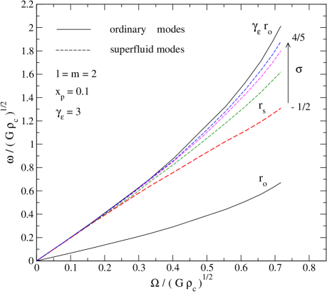
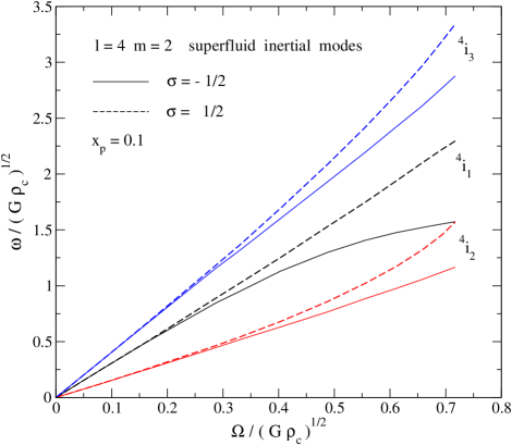
Figure 1: This figure shows the frequencies of the axial-led inertial modes and their dependence on the star’s spin and the symmetry energy $\sigma$ for the sequence of rotating models A with proton fraction $x_{\mathrm{p}}=0.1$ and entrainment parameter $\bar{\varepsilon}=2/3$. The mode-frequencies and the stellar angular velocity are given in units of $\sqrt{G\rho_{c}}$, where $G$ is the gravitational constant and $\rho_{c}$ the central mass density. The mode-frequencies are determined in the frame of the rotating star. In the left panel, we show the ordinary $\rm r_{o}$-mode and the superfluid $\rm r_{\mathrm{s}}$-modes for different values of $\sigma$ in the range $-1/2\leq\sigma\leq 4/5$. For fast rotating models, $\Omega/\sqrt{G\rho_{c}}>0.25$, the $\rm r_{s}$-mode deviates from the simple slow-rotation relation (61), where $\gamma_{\varepsilon}=1/(1-\bar{\varepsilon})=3$, because of the symmetry energy. In the right panel we show three $l=4,m=2$ superfluid inertial modes for $\sigma=-0.5$ and $\sigma=0.5$. These results also show a clear dependence on the symmetry energy. It is worth noticing that, for the non-stratified models A the ordinary inertial modes are equal to the results for single fluid $N=1$ polytropes, where $N$ is the polytropic index.

6 Results

In this section we present the result from the first ever time-evolution study of perturbed, rapidly rotating, superfluid stars. The main aim is to explore how fast rotation, symmetry energy and entrainment affect the non-axisymmetric oscillation modes.

6.1 The evolution code

The evolution problem for equations (16)–(19) is intrinsically a three dimensional problem. As already mentioned, the Fourier decomposition of the azimuthal degree of freedom, identifying specific $m$-modes, reduces the problem to two spatial dimensions. In spherical coordinates, we could then evolve this system of equations on a two-dimensional grid based on the coordinates $r$ and $\theta$. However, instead of using $r$ we adopt a new radial coordinate $x=x(r,\theta)$, fitted to surfaces of constant pressure (Jones et al., 2002; Passamonti et al., 2009). This leads to an easier implementation of the surface boundary conditions. As we are working in the time domain, the various mode frequencies are extracted by a Fast Fourier Transformation (FFT) of the time evolved perturbation variables.

The numerical code for superfluid neutron stars extends the single fluid code developed by Passamonti et al. (2009). In fact, with our chosen variables the Euler equation (16) and the mass conservation equation (18) are identical to the single fluid case. We have thus extended the previous code by adding equations (17) and (19), together with the appropriate boundary conditions. The main elements of the code are the use of a Mac-Cormack algorithm, a second order accurate numerical scheme both in space and time, and the implementation of a fourth-order Kreiss-Oliger numerical dissipation, which stabilizes the simulations against spurious high frequency oscillations. The performance of the final code is practically identical to that of the single fluid code, see Passamonti et al. (2009) for details.

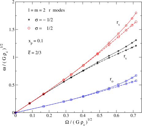
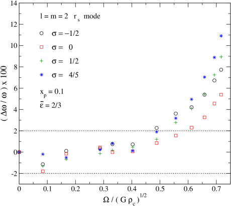
Figure 2: In this figure we compare our rotating frame frequencies for the r-modes with the slow rotation results of  Haskell et al. (2009), which include $\mathcal{O}\left(\Omega^{3}\right)$ corrections. In the left panel, we show the $l=m=2$ $\rm r_{s}$ and $\rm r_{o}$-mode frequencies for the rotating models A with $\sigma=\pm 1/2$, proton fraction $x_{\mathrm{p}}=0.1$, and entrainment parameter $\bar{\varepsilon}=2/3$. Our numerical results are shown as solid lines, while the frequencies of Haskell et al. (2009) are represented by dashed lines. The right panel provides the relative error between the $\rm r_{s}$-mode frequencies calculated with the two methods, where the dotted lines denote the 2% level. The results show that the calculated frequencies agree to better than 2% up to a stellar angular velocity of $\Omega/\sqrt{G\rho_{c}}\approx 0.4$.

6.2 Initial Data

In a time domain study, the initial perturbations can be chosen to excite specific parts of the spectrum. Of course, a strict selection of oscillation modes requires the determination of eigenfunctions to be used as initial data. To achieve this, one would have to either solve the frequency domain version of the perturbation equations (16)–(19) or perform an eigenfunction recycling study of the time evolutions (Stergioulas et al., 2004; Dimmelmeier et al., 2006). In this work we use neither of these strategies. We are interested in a multi-mode analysis where many oscillation modes are excited in each simulation. As discussed by Passamonti et al. (2009), this is easily achieved by the use of initial perturbations with an arbitrary radial profile and an angular dependence appropriate for the general class of eigenfunction. For the radial part we typically use a Gaussian distribution. Meanwhile the angular functions are inspired by slow-rotation results.

Type I parity perturbations are generally excited with the following mass density and proton fraction perturbations:

$$\delta\rho = A_{0}\,\exp{\left[-\left(\frac{r-r_{0}}{qR\left(\theta\right)}\right)^{2}\right]}Y_{ll}\left(\theta,\phi\right)\,,$$ (57)

$$\delta\chi_{\mathrm{p}} = A_{1}\,\exp{\left[-\left(\frac{r-r_{0}}{qR\left(\theta\right)}\right)^{2}\right]}Y_{ll}\left(\theta,\phi\right)\,,$$ (58)

where $A_{0}$ and $A_{1}$ are two arbitrary constants that determine the initial values of $\delta\rho$ and $\delta\chi_{\mathrm{p}}$ on the star’s surface. The stellar radius at polar angle $\theta$ is denoted by $R\left(\theta\right)$, and the parameters $r_{0}$ and $q$ respectively determine the centre of the Gaussian profile and its width. The $l=m$ spherical harmonic $Y_{ll}\left(\theta,\phi\right)$ approximates the typical angular behaviour of a polar mode in a spherical star. For simplicity, all other perturbation variables are set to zero to complete the initial data.

For Type II parity perturbations we use the following initial data for the vector fields $\mathbf{f}$ and $\mathbf{D}$:

$$\mathbf{f} = \rho\,\exp{\left[-\left(\frac{r-r_{0}}{qR\left(\theta\right)}\right)^{2}\right]}Y_{ll}^{B}\left(\theta,\phi\right)\,,$$ (59)

$$\mathbf{D} = x_{\mathrm{p}}\left(1-x_{\mathrm{p}}\right)\rho\,\exp{\left[-\left(\frac{r-r_{0}}{qR\left(\theta\right)}\right)^{2}\right]}Y_{ll}^{B}\left(\theta,\phi\right)\,,$$ (60)

Here $Y_{ll}^{B}\left(\theta,\phi\right)$ is a magnetic spherical harmonic (Thorne, 1980). The remaining perturbations are set to vanish on the initial time slice.

6.3 Inertial modes

Let us first consider the inertial modes which in a superfluid star split (more or less clearly depending on the equation of state) into ordinary and superfluid modes. In the first class, the perturbed fluid elements of the two components oscillate in phase, whereas for the superfluid modes they pulsate in counter-phase. As for single fluid stars, each inertial mode can be classified by its parity as an axial-led or polar-led inertial mode (Lockitch & Friedman, 1999). Among the axial-led inertial modes, the r-modes form a well defined sub-set. They are the only modes that are purely axial in the slow-rotation limit. In stratified neutron stars, only the co-moving r-mode exists. The counter-moving mode is no longer purely axial, but acquires a polar component already at leading order in the rotation (Haskell et al., 2009). In a non-stratified neutron star, on the other hand, the ordinary and superfluid degrees of freedom are completely decoupled and a purely axial counter-moving r-mode exists (Andersson et al., 2008; Haskell et al., 2009).

Up to $\mathcal{O}\left(\Omega\right)$, the frequencies of the superfluid and ordinary inertial modes are related according to (Prix et al., 2004):

$$\omega_{s}\simeq\gamma_{\varepsilon}\,\omega_{o}\,,$$ (61)

where $\gamma_{\varepsilon}\equiv(1-\bar{\varepsilon})^{-1}$. It makes sense, as a first step, to investigate to what extent the inertial-mode frequencies deviate from this simple scaling law in the case of rapid rotation. To do this, we consider model A with fixed entrainment parameter $\bar{\varepsilon}=2/3$ and proton fraction $x_{\mathrm{p}}=0.1$. For the symmetry energy term we consider four different values $\sigma=-1/2,0,1/2,4/5$. The results are shown in figure 1. In the left panel we show the $l=m=2$ ordinary and superfluid r-modes. The ordinary $\rm r_{o}$ mode is represented by a solid line and the expected frequency (61) of the superfluid $\rm r_{s}$ mode is also indicated. Our results show that the $\rm r_{s}$ mode frequencies for different values of $\sigma$ agree well with equation (61) roughly up to a stellar rotation $\Omega/\sqrt{G\rho_{c}}\simeq 0.2$. For faster rotation, the $\rm r_{s}$-mode frequency depends strongly on the symmetry energy.

In order to confirm these results, we also considered the superfluid r-modes within the slow-rotation approximation (Haskell et al., 2009). The approximate results confirm that, even though one should expect the counter-moving inertial modes to approach (61) as $\sigma\to 1$, the relation does not hold perfectly even in the extreme limit.

Our results show that the $\rm r_{s}$-mode frequency remains closer to the values expected from equation (61) for larger $\sigma$. Similar behaviour is noted for other inertial modes. In the right panel of figure 1, we show three $l=4$, $m=2$ axial-led inertial modes for $\sigma=\pm 1/2$. The dependence on the symmetry energy term is distinguishable beyond $\Omega/\sqrt{G\rho_{c}}\approx 0.25$ also for these modes. These results can be understood from a local plane-wave analysis, see Appendix A for a detailed discussion.

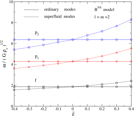
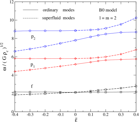
Figure 3: This figure illustrates the dependence of the $l=m=2$ acoustic modes on the entrainment parameter $\bar{\varepsilon}$ for two non-rotating stellar models, the non-stratified $\rm B^{NS}$ model (left panel) and the stratified B0 model (right panel). Solid and dashed lines represent oscillation modes where neutrons and protons move, respectively, in phase (ordinary modes) and counter-phase (superfluid modes). The spectrum of the B0 model shows some avoided crossings. Avoided crossings are expected in a stratified neutron star as the co- and counter-moving degrees of freedom are coupled.

We can also compare our results to the superfluid r-mode frequencies calculated by Haskell et al. (2009), who worked in the slow-rotation approximation keeping terms up to $\mathcal{O}\left(\Omega^{3}\right)$. The $l=m=2$ $\rm r_{s}$ frequency is then given by

$$\omega_{\mathrm{s}}=c_{0}\,\Omega+c_{2}\,\Omega^{3}\,,$$ (62)

where $c_{0}$ and $c_{2}$ are constants that depend on the stellar model and the multipole of the modes. The first coefficient has the well known analytical expression:

$$c_{0}=\gamma_{\varepsilon}\,\frac{2m}{l\left(l+1\right)}\,,$$ (63)

while $c_{2}$ is given in closed form by Haskell et al. (2009). For the $l=m=2$ $\rm r_{s}$-mode of a model A star with $\bar{\varepsilon}=2/3$ and $x_{\mathrm{p}}=0.1$, we have $c_{0}=2$ and the values for $c_{2}$ given in Table 3. In figure 2, we compare the $\rm r_{s}$-mode frequencies extracted from our evolutions to those determined analytically by Haskell et al. (2009) for different values of the symmetry energy. In the left panel, we show how the $\rm r_{s}$-mode frequency depends on the star’s rotation for two selected models with $\sigma=\pm 1/2$. The right panel shows the relative error between the frequencies obtained with the two methods. The agreement is better than three percent up to $\Omega/\sqrt{G\rho_{c}}\approx 0.55$, which corresponds to a rapidly rotating star with $\Omega/\Omega_{K}\approx 0.77$ (see Table 1). For faster rotation, the errors become larger and reach eleven per cent near the mass shedding limit. In order to improve the accuracy, the slow-rotation analysis would need to consider higher order corrections. This may be prohibitively difficult.

Table 3: The coefficient $c_{2}$ required in equation (62) for the $l=m=2$ superfluid r-mode. The values of $c_{2}$ are given in the units used in Haskell et al. (2009), i.e. $GM/R^{3}$. Here we have used the mass $M$ and the radius $R$ for the non-rotating model A0, with $\bar{\varepsilon}=2/3$ and $x_{\mathrm{p}}=0.1$.

$\sigma$	$c_{2}$
$-0.5$	$-1.052$
0.0	0.452
0.5	0.956
0.8	1.123

The dependence of the superfluid inertial modes on the proton fraction is very weak for model A neutron stars. That this should be expected can be seen from equation (81). To confirm this we have evolved the fast rotating model A8 with $x_{\mathrm{p}}=0.01$. The frequencies for this model differ by less than one percent from the $x_{\mathrm{p}}=0.1$ case.

6.4 Acoustic modes

Let us now study the effects of entrainment and symmetry energy on the fundamental and pressure modes of a superfluid star. The acoustic mode spectrum is characterized by the usual two classes of ordinary (co-moving) and superfluid (counter-moving) modes. We will focus on the quadrupole $l=m=2$ modes. These are the modes that tend to be the most relevant for gravitational-wave studies.

First we consider the oscillations of two non-rotating equilibrium configurations, the non-stratified $\rm B^{NS}$ model and the stratified B0 model described in Section 5.2. In figure 3, we show the variation of the fundamental quadrupole mode and the first two quadrupole pressure modes with the entrainment parameter $\bar{\varepsilon}$. In order to determine the co- and counter-moving character of a mode, we have first reconstructed the time variation of the component velocities $\mathbf{v_{\mathrm{x}}}$ from the primary dynamical variables $\mathbf{f}$ and $\mathbf{D}$. Post processing the numerical evolution data, we have determined the velocity components using the eigenfunction extraction code developed by Stergioulas et al. (2004) and Dimmelmeier et al. (2006). For any mode, we have then compared the velocity eigenfunctions of the two fluid components and determined whether they oscillate in phase or counter-phase. In figure 3, the solid lines represent modes that oscillate in phase, while dashed lines correspond to modes that pulsate in counter-phase. In absence of composition gradients (model $\rm B^{NS}$ in the left panel of figure 3), the co-moving and counter-moving degrees of freedom are completely decoupled and the spectrum does not exhibit any interaction between ordinary and superfluid modes. They are actually related by the simple expression, cf. (81),

$$\omega_{\mathrm{s}}\simeq\sqrt{\gamma_{\varepsilon}}\,\omega_{\mathrm{o}}\,.$$ (64)

The spectrum of stratified superfluid stars is more interesting. From the right panel of figure 3, we note that the coupling between “ordinary” and “superfluid” perturbations generates avoided crossings, where the oscillation phase of the mode changes at (roughly) $\bar{\varepsilon}=0$. This behaviour is more evident in the ordinary and superfluid pressure modes. From our data there does not appear to be an avoided crossing for the fundamental mode. However, the region where this crossing should take place is difficult to resolve with our evolutions. We have tried different initial data sets but only managed to find a single f-mode at $\bar{\varepsilon}=0$. Nonradial oscillations of the $\rm B^{NS}$ and B0 models have already been studied by Prix & Rieutord (2002), although not within the Cowling approximation. A direct comparison with their results is not possible since the Cowling approximation can introduce a 15-20$\%$ error in the f-mode frequencies. However, the qualitative behaviour of the acoustic spectrum in the two studies is clearly similar.

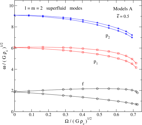
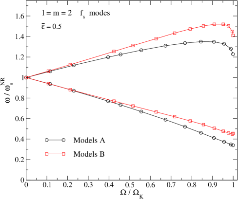
Figure 4: This figure shows the rotational splitting of the $l=m=2$ non-axisymmetric modes (in the reference frame of the rotating star) for the two sequences of rotating models A and B. In the left panel, we show the dimensionless frequencies of the superfluid f-mode and the first two counter-moving p-modes for models A with $\sigma=0$ and $\bar{\varepsilon}=0.5$. In the right panel, we compare the superfluid f-modes of these A models with the models B having $\bar{\varepsilon}=0.5$. In this panel, the star’s angular velocity is normalized (the horizontal axis) with the mass-shedding limit $\Omega/\Omega_{K}$, while the mode-frequency is divided by the superfluid f-mode frequency of the non-rotating star $\omega_{\mathrm{s}}^{\rm{NS}}$ (the vertical axis).

In order to investigate the effect of entrainment on the rotational splitting of the non-axisymmetric acoustic modes we consider a sequence of A models with $\sigma=0$ and models B. In figure 4, we show results corresponding to the $l=m=2$ acoustic modes in the $\bar{\varepsilon}=0.5$ case. For the generic initial data given by equations (57)–(58) many oscillation modes are excited in the numerical simulations. By studying their eigenfunctions we can track individual modes from the non-rotating model up to the mass shedding limit. An example is illustrated in the left panel of figure 4, where the rotating frame frequencies of the superfluid f-mode and the first two p-modes are shown for the A models. The counter-moving f_s mode exhibits a larger rotational splitting compared to the two pressure modes. In the right panel of figure 4, we compare instead the normalized frequencies of the superfluid f-mode, namely $\omega/\omega^{\rm{NR}}_{\mathrm{s}}$, for models A and B. The horizontal-axis of this figure represents the stellar rotation divided by the maximal angular velocity $\Omega_{K}$. The results in the figure show that, even though the two classes of models have the same value of the entrainment parameter, the non-axisymmetric splitting of the f_s mode is quite different in the two cases. This is particularly clear in the rapid rotation regime. Meanwhile, the two $\rm f_{\mathrm{s}}$ modes have very similar frequencies for $\Omega\mathrel{\hbox{\hbox to0.0pt{\hbox{\lower 4.0pt\hbox{$\sim$}}\hss}\hbox{$<$}}}0.25~{}\Omega_{K}$.

It is instructive to explore the slow-rotation regime to see if there is a simple relation between the $\rm f_{\mathrm{s}}$ mode frequencies and the entrainment. To this end, we determine the $\rm f_{\mathrm{s}}$ mode frequencies for models A and B with $-0.7\leq\bar{\varepsilon}\leq 0.7$. In the left panel of figure 5, the variation of the $\rm f_{\mathrm{s}}$ mode frequency with $\bar{\varepsilon}$ is shown for models A. It is useful to recall that these models have $\sigma=0$ by construction. All modes have been normalized to the f-mode frequency of the non-rotating star. The rotational splitting of the modes strongly depends on the parameter $\bar{\varepsilon}$. In order to quantify the effect, we approximate the dimensionless mode-frequency $\hat{\omega}_{\mathrm{s}}=\omega_{\mathrm{s}}/\sqrt{G\rho_{c}}$ (see Appendix A) by a second order polynomial in $\hat{\Omega}=\Omega/\sqrt{G\rho_{c}}$,

$$\hat{\omega}_{\mathrm{s}}=\hat{\omega}_{\mathrm{s}}^{\rm{NR}}+c_{1}\left(\varepsilon,\sigma,m\right)\hat{\Omega}+c_{2}\left(\varepsilon,\sigma,m\right)\hat{\Omega}^{2}+\mathcal{O}\left(\hat{\Omega}^{3}\right)\,,$$ (65)

where $\hat{\omega}^{\rm{NR}}_{\mathrm{s}}=\omega^{\rm{NR}}_{\mathrm{s}}/\sqrt{G\rho_{c}}$ is the superfluid mode frequency of the non-rotating star, while $c_{1}$ and $c_{2}$ are two parameters that we fit to the numerical data. In general, these parameters are functions of the entrainment, the symmetry energy and the multipole $m$ of the mode. Since this is inherently a slow-rotation approximation, we will only consider rotating models with $\Omega\mathrel{\hbox{\hbox to0.0pt{\hbox{\lower 4.0pt\hbox{$\sim$}}\hss}\hbox{$<$}}}0.375~{}\Omega_{K}$. An accurate description of the spectrum for more rapidly rotating models would require higher order fitting functions. In the right panel of figure 5, we show the dependence of $\hat{\omega}^{\rm{NR}}_{\mathrm{s}}$ and $c_{1}$ on

$$\gamma_{\varepsilon}=\left(1-\bar{\varepsilon}\right)^{-1}\,,$$ (66)

for Models A. We have defined $c_{1}^{r}$ and $c_{1}^{p}$ for retrograde and prograde modes, respectively. If we assume that a perturbation variable is proportional to $e^{i\left(\omega t+m\phi\right)}$, modes with positive (negative) $m$ move retrograde (prograde) with respect to the stellar rotation.

For non-stratified and non-rotating stellar models, equation (81) suggests that the superfluid and ordinary f-mode frequencies are related according to

$$\hat{\omega}_{\mathrm{s}}^{\rm{NR}}=\sqrt{\gamma_{\varepsilon}}\,\chi(\sigma,x_{\mathrm{p}})\,\hat{\omega}_{\mathrm{o}}^{\rm{NS}}\,,$$ (67)

where $\chi$ is a function of $\sigma$ and $x_{\mathrm{p}}$ that, in general, depends on the EoS. For models A, this function is given explicitly by

$$\chi^{2}\equiv\frac{\left(1+\sigma\right)\left(1-x_{\mathrm{p}}\right)}{1-\left(1+\sigma\right)x_{\mathrm{p}}}\,.$$ (68)

Since we consider a sequence of models with $\sigma=0$ it follows that $\chi=1$. We test the accuracy of equation (67) against the f-mode frequencies for models A shown in figure 5. Fitting our numerical data to a function of form

$$a\gamma_{\varepsilon}^{b}\,,$$ (69)

we obtain the values for $a$ and $b$ listed in Table 4. These results are in very good agreement with the analytical formula (67). In fact, the ordinary f-mode frequency determined from our code is $\hat{\omega}_{\mathrm{o}}=1.867$, which agrees to better than $0.06\%$ with the fitted value. Equation (67) also provides an accurate representation for the f-mode of the B models. In this case, the numerical evolutions lead to $\hat{\omega}_{\mathrm{o}}=2.1598$, which is within the error bar of the fitted result, see Table 4. It should be noted that we do not have a simple analytic expression for $\chi$ in the case of the B models. Our results suggest that $\chi$ is only weakly dependent on the entrainment also for this equation of state.

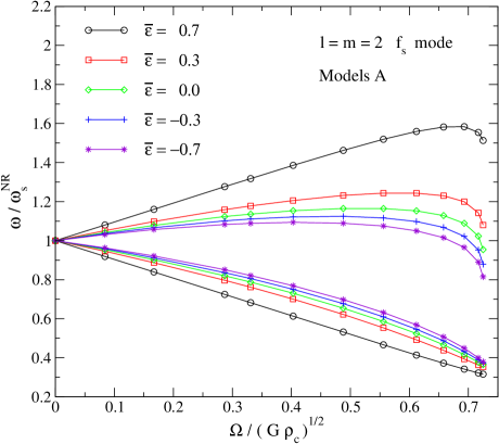
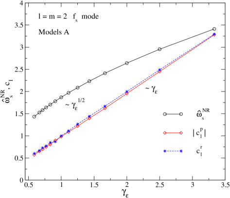
Figure 5: The effect of the entrainment parameter $\bar{\varepsilon}$ on the rotational splitting is shown in this figure. For the sequence of stellar models A with $\sigma=0$, the left panel displays the rotating frame frequencies of the $l=m=2$ superfluid modes for several values of $\bar{\varepsilon}$. The mode-frequencies are normalized with the superfluid f-mode frequencies of the non-rotating star $\omega_{\mathrm{s}}^{\rm{NR}}$. In the right panel, we show how the dimensionless frequency $\hat{\omega}_{\mathrm{s}}^{\rm{NR}}=\omega_{\mathrm{s}}/\sqrt{G\rho_{c}}$ and the two splitting parameters $c_{1}^{r}$ and $c_{1}^{p}$ of equation (65) depend on the entrainment parameter $\gamma_{\varepsilon}=\left(1-\bar{\varepsilon}\right)^{-1}$. The superscripts $r$ and $p$ for the parameters $c_{1}^{r}$ and $c_{1}^{p}$ denote retrograde and prograde modes, respectively. The quantities $c_{1}^{r}$ and $c_{1}^{p}$ have been determined by a fit to the superfluid f-mode frequencies for models A up to $\Omega\mathrel{\hbox{\hbox to0.0pt{\hbox{\lower 4.0pt\hbox{$\sim$}}\hss}\hbox{$<$}}}0.375~{}\Omega_{K}$.

Let us now consider the rotational corrections to the counter-moving f-mode frequency, cf. equation (65). We find that we can still use the fitting function (69) for the parameter $c_{1}$. This leads to the results given in Table 4. These results suggest that the rotational splitting parameter $c_{1}$ depends linearly on the entrainment parameter $\gamma_{\varepsilon}$ for both models A and B. This is also clear from the results in Figure 5. To describe the quantities $c_{2}^{r}$ and $c_{2}^{p}$, we instead used the following fitting function:

$$\frac{a+b\,\gamma_{\varepsilon}}{\hat{\omega}^{\rm{NR}}_{\mathrm{s}}}\,.$$ (70)

The results for $a$ and $b$ are given in Table 4. Despite the fact that models B are stratified, the $\rm f_{\mathrm{s}}$ mode seems to maintain the same dependence on the entrainment as for the non-stratified models A in the slow rotation regime.

Building on this, let us try to understand the dependence on the symmetry energy. To do this we consider the sequence of rotating stellar models A and take the symmetry energy in the range $-1/2\leq\sigma\leq 1/2$. Meanwhile the proton fraction and the entrainment are kept constant at $x_{\mathrm{p}}=0.1$ and $\bar{\varepsilon}=2/3$, respectively. The $\rm f_{\mathrm{s}}$ mode dependence on the stellar spin (for some of these models) is shown in figure 6. In the figure, we have normalized the mode-frequencies to the f-mode frequency of the non-rotating model. The results show that the rotational splitting of the $l=m=2$ superfluid f-mode decreases for larger values of the symmetry energy. In the slow rotation regime, we can study this effect by fitting the numerical data using equation (65). Adding the dependence on the symmetry energy to our previous results, we now use the fitting function

$$\hat{\omega}_{\mathrm{s}}=\sqrt{\gamma_{\varepsilon}}\,\chi(\sigma,x_{\mathrm{p}})\,\hat{\omega}_{\mathrm{o}}^{\rm{NS}}+\gamma_{\varepsilon}\,\tilde{c}_{1}\left(\sigma,m\right)\hat{\Omega}+\tilde{c}_{2}\left(\varepsilon,\sigma,m\right)\hat{\Omega}^{2}+\mathcal{O}\left(\hat{\Omega}^{3}\right)\,,$$ (71)

where $\tilde{c}_{2}$ is in general different from $c_{2}$, and we have assumed that $\tilde{c}_{1}$ is a function of only $\sigma$ and $m$. First we consider the non-rotating case, using the ordinary frequency of the f-mode $\hat{\omega}_{\mathrm{o}}^{\rm{NS}}$ as a fitting parameter. The fitted result agrees with the numerical value determined from the simulations to better than $0.04\%$. Empirically we find that the parameters $\tilde{c}_{1}$ can be approximated by the function:

$$\frac{\gamma_{\varepsilon}\,\tilde{a}\,\chi^{\tilde{b}}}{\hat{\omega}_{\mathrm{s}}^{\rm{NR}}}\,,$$ (72)

The determined values for $\tilde{a}$ and $\tilde{b}$ for model A are given in Table 5. We find that the parameter $\tilde{c}_{2}$ assumes less regular values. They can be fitted with a quadratic polynomial in $\sigma$, but the fits are not very accurate. Hence, we do not provide any of those results here. However, as our main aim was to provide an approximate description of the rotational splitting of the quadrupole superfluid f-mode, reliable values for the coefficient $\tilde{c}_{1}$ should be sufficient.

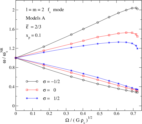
Figure 6: This figure shows the effect of the symmetry energy on the rotational splitting of the quadrupole superfluid f-mode. The data in the figure corresponds to stellar models A with constant proton fraction $x_{\mathrm{p}}=0.1$ and entrainment $\bar{\varepsilon}=2/3$. The symmetry energy takes the three values $\sigma=-0.5,0,0.5$.

Table 4: This table provides the values of the fitting parameters $a\pm\Delta a$ and $b\pm\Delta b$ from equations (69) and (70) for the superfluid f-mode of the non-rotating star, i.e. $\hat{\omega}^{\rm{NR}}_{\mathrm{s}}$, and the splitting coefficients $c_{k}^{r}$ and $c_{k}^{p}$ with $k=1,2$ for the retro- and pro-grade $\rm f_{\mathrm{s}}$ modes. In the fits we have used the stellar models A and B with $\Omega\mathrel{\hbox{\hbox to0.0pt{\hbox{\lower 4.0pt\hbox{$\sim$}}\hss}\hbox{$<$}}}0.375~{}\Omega_{K}$.

	Models	$a$	$\Delta a$	$b$	$\Delta b$
$\hat{\omega}_{\mathrm{s}}^{\rm{NR}}$	A	1.8686	$2.1\times 10^{-4}$	0.5000	$1.5\times 10^{-4}$
$c_{1}^{r}$	A	1.0034	$4.7\times 10^{-3}$	0.9896	$5.4\times 10^{-3}$
$c_{1}^{p}$	A	-0.9744	$1.7\times 10^{-3}$	1.0072	$2.1\times 10^{-3}$
$c_{2}^{r}$	A	-0.5306	$1.7\times 10^{-2}$	0.1513	$1.1\times 10^{-2}$
$c_{2}^{p}$	A	-0.5203	$4.4\times 10^{-3}$	0.1570	$2.8\times 10^{-3}$
$\hat{\omega}_{\mathrm{s}}^{\rm{NR}}$	B	2.1597	$8.6\times 10^{-4}$	0.4987	$1.0\times 10^{-3}$
$c_{1}^{r}$	B	1.0091	$3.4\times 10^{-3}$	0.9998	$7.6\times 10^{-3}$
$c_{1}^{p}$	B	-0.9837	$3.8\times 10^{-3}$	1.0059	$8.7\times 10^{-3}$
$c_{2}^{r}$	B	-0.1421	$7.8\times 10^{-3}$	-0.0998	$6.6\times 10^{-3}$
$c_{2}^{p}$	B	-0.1461	$1.2\times 10^{-2}$	0.1106	$1.1\times 10^{-2}$

Table 5: This table provides the values of the fitting parameters $\tilde{a}\pm\Delta\tilde{a}$ and $\tilde{b}\pm\Delta\tilde{b}$ from equation (72). They describe the splitting functions $\tilde{c}_{1}^{r}$ and $\tilde{c}_{1}^{p}$ for the $l=m=2$ superfluid f-mode. The labels $r$ and $p$ denote retro- and pro-grade $\rm f_{\mathrm{s}}$ modes, respectively. In the fits we have used results for models A with $\Omega\mathrel{\hbox{\hbox to0.0pt{\hbox{\lower 4.0pt\hbox{$\sim$}}\hss}\hbox{$<$}}}0.375~{}\Omega_{K}$.

	Models	$\tilde{a}$	$\Delta\tilde{a}$	$\tilde{b}$	$\Delta\tilde{b}$
$\tilde{c}_{1}^{r}$	A	0.3721	$1.1\times 10^{-3}$	-0.985	$1.5\times 10^{-2}$
$\tilde{c}_{1}^{p}$	A	-0.3045	$1.5\times 10^{-3}$	-1.024	$2.0\times 10^{-2}$

7 Conclusions

In this paper we have considered, for the first time, the oscillations of a superfluid neutron star as an initial-value problem. Using time evolutions of the relevant linearised equations we studied non-axisymmetric oscillations of rapidly rotating superfluid neutron stars. We considered perturbations of axisymmetric background configurations in Newtonian gravity and accounted for the presence of superfluid components via the standard two-fluid model. Within the Cowling approximation, we were able to carry out evolutions for uniformly rotating stars up to the mass-shedding limit. Our results represent the first detailed analysis of superfluid neutron star oscillations in the fast rotation regime, where the star is significantly deformed by the centrifugal force.

For simplicity, we focused on background models such that the two fluids (superfluid neutrons and protons) co-rotate, are in $\beta$-equilibrium and coexist in all the volume of the star. Two different analytical model equations of state were considered. The models were chosen to represent relatively simple generalizations of single fluid, polytropic stars. We investigated the effects of entrainment, rotation and symmetry energy on various non-radial oscillation modes of these models. Our results show that entrainment and symmetry energy can have a significant effect on the rotational splitting of non-axisymmetric modes. In particular, the symmetry energy modifies the inertial mode frequencies considerably in the regime of fast rotation.

The perturbative time-evolution framework provides a useful tool that should allow us to consider more realistic (and by necessity complicated) neutron star models in the future. The clear advantage over frequency-domain studies is that it is straightforward to study oscillations corresponding to eigenfunctions with a complex set of rotational couplings. This is particularly useful in the rapid rotation regime. The obvious downside is that time evolutions can never provide the “complete” mode spectrum of the star. Initial data has to be chosen in such a way that the oscillations of interest are excited at a significant level. It is difficult to, without prior knowledge, find initial data that excites only a few modes. In many cases this is, however, less relevant. The main question is if one can extract accurate information regarding the nature of the star’s oscillations from the numerical data. The results we have presented demonstrate that this is, undoubtedly, the case. Hence, it is relevant to develop the perturbative evolution framework further. We are currently considering more general background models, with a relative velocity between the two fluid components. We are also adding the dissipative coupling associated with mutual friction to the code. Once these features are incorporated we will be able to consider (obviously still at a basic level) the dynamics associated with the superfluid two-stream instability (Andersson et al., 2003, 2004) and the possible relation with pulsar glitches (see Glampedakis & Andersson, 2008, for a recent discussion). This is a very exciting prospect. Looking further ahead, we would like to add layering to the stellar model by introducing both an elastic crust and distinct superfluid/normal regions. There are challenges associated with these aspects, but there is no reason why these developments should be prohibitively difficult.

Appendix A Local Analysis

In this Appendix we carry out a local analysis of the perturbation equations (16)–(19). The aim is to obtain understand the superfluid oscillation spectrum and its dependence on parameters like the proton fraction, the entrainment and the symmetry energy. Since we are only interested in a qualitative picture we focus on the non-stratified $N=1$ polytropic model A (see Section 5.1). For this sequence of models, the ordinary and superfluid perturbation variables are decoupled. We consider only the “superfluid” perturbations as the dispersion relations for the ordinary modes are well known, see for example (Unno et al., 1989). For model A the superfluid perturbation equations (17) and (19) can be written

$$\gamma_{\varepsilon}^{-1}\,\partial_{t}\mathbf{D} = -\alpha^{2}\nabla\delta\chi_{\mathrm{p}}-2\mathbf{\Omega}\times\mathbf{D}\,,$$ (73)

$$\partial_{t}\delta\chi_{\mathrm{p}} = -\nabla\cdot\mathbf{D}-\mathbf{f}\cdot\nabla x_{\mathrm{p}}\,,$$ (74)

where we have defined

$$\gamma_{\varepsilon} \equiv \left(1-\bar{\varepsilon}\right)^{-1}\,,$$ (75)

$$\alpha^{2} \equiv \left[\,x_{\mathrm{p}}\left(1-x_{\mathrm{p}}\right)\rho\right]\frac{1}{\rho}\left.\frac{\partial\beta}{\partial x_{\mathrm{p}}}\right|_{\rho}=\frac{c_{s}^{2}\left(1+\sigma\right)\left(1-x_{\mathrm{p}}\right)}{\left[1-\left(1+\sigma\right)x_{\mathrm{p}}\right]}\,,$$ (76)

and where the speed of sound for an $N=1$ polytrope is given by $c_{s}^{2}=2K\rho$. Now we assume that the perturbation variables behave as plane waves, i.e. we introduce an $e^{i\left(\omega t-\mathbf{k}\cdot\mathbf{r}\right)}$ dependence for all perturbations into equations (73)–(74). Here $\omega$ and $\mathbf{k}$ are the frequency and wave vector, respectively. The characteristic polynomial of the resulting equations is then given by

$$\hat{\omega}^{4}-\left(\hat{\eta}^{2}\gamma_{\varepsilon}+4\gamma_{\varepsilon}^{2}\hat{\Omega}^{2}\right)\hat{\omega}^{2}+\hat{\eta}^{2}\gamma_{\varepsilon}^{3}\left(2\hat{\mathbf{\Omega}}\cdot\hat{\mathbf{k}}\right)^{2}=0\,,$$ (77)

where $\hat{\mathbf{k}}$ is the unit wave vector and we have defined the following dimensionless variables:

$$\hat{\Omega} \equiv \frac{\Omega}{\sqrt{G\rho_{c}}}\,,$$ (78)

$$\hat{\omega} \equiv \frac{\omega}{\sqrt{G\rho_{c}}}\,,$$ (79)

$$\hat{\eta} \equiv \frac{\alpha k}{\sqrt{G\rho_{c}}}\,.$$ (80)

The quantities $M$ and $R$ denote the mass and radius of a non-rotating stellar model, respectively. In the slow-rotation approximation, we can assume that $\hat{\Omega}<<\hat{\eta}$. Equation (77) then have the following solutions [up to $\mathcal{O}\left(\Omega^{3}\right)$]

$$|\hat{\omega}_{1}| \simeq \sqrt{\gamma_{\varepsilon}}\,\hat{\eta}+\frac{2\,\gamma_{\varepsilon}^{3/2}}{\hat{\eta}}\left[\hat{\Omega}^{2}-\left(\hat{\mathbf{\Omega}}\cdot\hat{\mathbf{k}}\right)^{2}\right]\,,$$ (81)

$$|\hat{\omega}_{2}| \simeq \gamma_{\varepsilon}\,2\hat{\mathbf{\Omega}}\cdot\hat{\mathbf{k}}-\frac{4\,\gamma_{\varepsilon}^{2}}{\hat{\eta}^{2}}\left[\hat{\Omega}^{2}-\left(\hat{\mathbf{\Omega}}\cdot\hat{\mathbf{k}}\right)^{2}\right]\hat{\mathbf{\Omega}}\cdot\hat{\mathbf{k}}\simeq\gamma_{\varepsilon}\,2\hat{\mathbf{\Omega}}\cdot\hat{\mathbf{k}}\left\{1-\frac{2\,\gamma_{\varepsilon}}{\hat{\eta}^{2}}\left[\hat{\Omega}^{2}-\left(\hat{\mathbf{\Omega}}\cdot\hat{\mathbf{k}}\right)^{2}\right]\right\}\,.$$ (82)

As an estimate we consider a non-rotating background model with an $N=1$ polytropic EoS. Using the definitions (76) and (80) we have

$$\hat{\eta}^{2}\simeq\frac{48}{\pi}\frac{\left(1+\sigma\right)\left(1-x_{\mathrm{p}}\right)}{\left[1-\left(1+\sigma\right)x_{\mathrm{p}}\right]}\left(\frac{R}{\lambda}\right)^{2}\,,$$ (83)

where $\lambda$ is the wavelength (related to the the wave vector according to $k=2\pi/\lambda$). In addition, we have replaced the speed of sound with its average value for an $N=1$ polytrope:

$$\langle c_{s}^{2}\rangle=\frac{3}{\pi^{2}}\frac{GM}{R}\,.$$ (84)

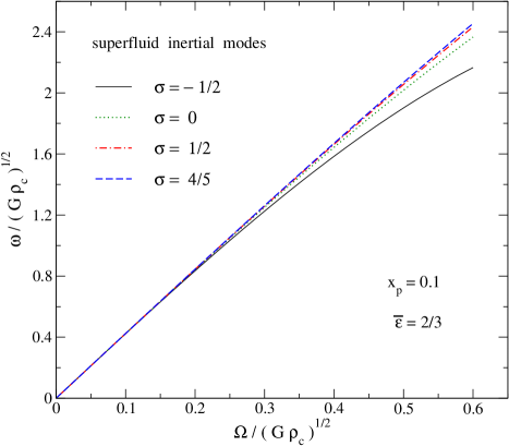
Figure 7: This figure shows the inertial mode frequencies estimated from the dispersion relation (81). We consider the four values of the symmetry energy term given in the legend. In equation (81), the correction term at $\mathcal{O}(\Omega^{3})$ leads to a dependence on $\sigma$ which is very similar to the behaviour seen for the numerically determined mode-frequencies, see figure 1 in the main text.

If we now assume that the wavelength of the mode is of the same order as the stellar radius, $\lambda=R$, equation (83) for $\hat{\eta}$ becomes

$$\hat{\eta}^{2}\simeq\frac{48}{\pi}\frac{\left(1+\sigma\right)\left(1-x_{\mathrm{p}}\right)}{\left[1-\left(1+\sigma\right)x_{\mathrm{p}}\right]}\,.$$ (85)

To get a qualitative picture, we consider parameter values $\bar{\varepsilon}=2/3$ and $x_{\mathrm{p}}=0.1$ and specify the angle between $\hat{\mathbf{\Omega}}$ and $\hat{\mathbf{k}}$ to be $\theta=\pi/4$. In figure 7, we show the positive frequency $\hat{\omega}_{\mathrm{s}}$ of equation (81) for different values of $\sigma$. The $\mathcal{O}\left(\Omega^{3}\right)$ correction term leads to a behaviour that resembles the global mode results shown in figure 1 in the main text.

References

- Andersson & Comer (2001) Andersson N., Comer G. L., 2001, MNRAS, 328, 1129
- Andersson & Comer (2006) Andersson N., Comer G. L., 2006, Classical and Quantum Gravity, 23, 5505
- Andersson et al. (2004) Andersson N., Comer G. L., Grosart K., 2004, MNRAS, 355, 918
- Andersson et al. (2002) Andersson N., Comer G. L., Langlois D., 2002, Phys. Rev. D, 66, 104002
- Andersson et al. (2003) Andersson N., Comer G. L., Prix R., 2003, Physical Review Letters, 90, 091101
- Andersson et al. (2004) Andersson N., Comer G. L., Prix R., 2004, MNRAS, 354, 101
- Andersson et al. (2008) Andersson N., Glampedakis K., Haskell B., 2008, ArXiv e-prints
- Andersson & Kokkotas (1998) Andersson N., Kokkotas K. D., 1998, MNRAS, 299, 1059
- Benhar et al. (2004) Benhar O., Ferrari V., Gualtieri L., 2004, Phys. Rev., D70, 124015
- Chamel (2006) Chamel N., 2006, Nuclear Physics A, 773, 263
- Chamel (2008) Chamel N., 2008, MNRAS, 388, 737
- Dimmelmeier et al. (2006) Dimmelmeier H., Stergioulas N., Font J. A., 2006, MNRAS, 368, 1609
- Epstein (1988) Epstein R. I., 1988, ApJ, 333, 880
- Glampedakis & Andersson (2008) Glampedakis K., Andersson N., 2008, ArXiv e-prints
- Hachisu (1986) Hachisu I., 1986, ApJSS, 61, 479
- Haskell et al. (2009) Haskell B., Andersson N., Passamonti A., 2009, ArXiv e-prints
- Hessels et al. (2006) Hessels J. W. T., Ransom S. M., Stairs I. H., Freire P. C. C., Kaspi V. M., Camilo F., 2006, Science, 311, 1901
- Ipser & Lindblom (1990) Ipser J. R., Lindblom L., 1990, ApJ, 355, 226
- Jones et al. (2002) Jones D. I., Andersson N., Stergioulas N., 2002, MNRAS, 334, 933
- Khalatnikov (1965) Khalatnikov I. M., 1965, An Introduction to the Theory of Superfluidity. Benjamin, New York
- Landau & Lifshitz (1959) Landau L. D., Lifshitz E. M., 1959, Fluid Mechanics, Course of Theoretical Physics Vol. 6. Pergamon, Oxford
- Lattimer & Prakash (2004) Lattimer J. M., Prakash M., 2004, Science, 304, 536
- Lattimer & Prakash (2007) Lattimer J. M., Prakash M., 2007, Phys. Rep., 442, 109
- Lee (1995) Lee U., 1995, A&A, 303, 515
- Lindblom & Mendell (2000) Lindblom L., Mendell G., 2000, Phys. Rev. D, 61, 104003
- Lockitch & Friedman (1999) Lockitch K. H., Friedman J. L., 1999, ApJ, 521, 764
- Mendell (1991a) Mendell G., 1991a, ApJ, 380, 515
- Mendell (1991b) Mendell G., 1991b, ApJ, 380, 530
- Page et al. (2006) Page D., Geppert U., Weber F., 2006, Nuclear Physics A, 777, 497
- Papaloizou & Pringle (1980) Papaloizou J. C., Pringle J. E., 1980, MNRAS, 190, 43
- Passamonti et al. (2009) Passamonti A., Haskell B., Andersson N., Jones D. I., Hawke I., 2009, MNRAS, 394, 730
- Prakash et al. (1988) Prakash M., Lattimer J. M., Ainsworth T. L., 1988, Physical Review Letters, 61, 2518
- Prix (2004) Prix R., 2004, Phys. Rev. D, 69, 043001
- Prix et al. (2002) Prix R., Comer G. L., Andersson N., 2002, A&A, 381, 178
- Prix et al. (2004) Prix R., Comer G. L., Andersson N., 2004, MNRAS, 348, 625
- Prix & Rieutord (2002) Prix R., Rieutord M., 2002, A&A, 393, 949
- Reisenegger & Goldreich (1992) Reisenegger A., Goldreich P., 1992, ApJ, 395, 240
- Samuelsson & Andersson (2007) Samuelsson L., Andersson N., 2007, MNRAS, 374, 256
- Shapiro & Teukolsky (1983) Shapiro S. L., Teukolsky S. A., 1983, Black holes, white dwarfs, and neutron stars. New York, Wiley-Interscience, 1983
- Stergioulas (2003) Stergioulas N., 2003, Living Reviews in Relativity, 6
- Stergioulas et al. (2004) Stergioulas N., Apostolatos T. A., Font J. A., 2004, MNRAS, 352, 1089
- Tassoul (1978) Tassoul J. L., 1978, Theory of rotating stars. Princeton University press, Princeton
- Thorne (1980) Thorne K. S., 1980, Reviews of Modern Physics, 52, 299
- Tilley & Tilley (1990) Tilley D. R., Tilley J., 1990, Superfluidity and Superconductivity. IOP, London
- Unno et al. (1989) Unno W., Osaki Y., Ando H., Saio H., Shibahashi H., 1989, Nonradial oscillations of stars. Tokyo: University of Tokyo Press, 1989, 2nd ed.
- Yoshida & Eriguchi (2004) Yoshida S., Eriguchi Y., 2004, MNRAS, 347, 575
- Yoshida & Lee (2003a) Yoshida S., Lee U., 2003a, MNRAS, 344, 207
- Yoshida & Lee (2003b) Yoshida S., Lee U., 2003b, Phys. Rev. D, 67, 124019