Fully discrete Galerkin schemes for the nonlinear and nonlocal Hartree equation

Abstract

We study the time dependent Hartree equation in the continuum, the semidiscrete, and the fully discrete setting. We prove existence-uniqueness, regularity, and approximation properties for the respective schemes, and set the stage for a controlled numerical computation of delicate nonlinear and nonlocal features of the Hartree dynamics in various physical applications.

2000 Mathematics Subject Classification. 35Q40, 35Q35, 35J60, 65M60, 65N30

Key words. Hartree equation, quantum many-body system, weakly nonlinear dispersive waves, Newtonian gravity, Galerkin theory, finite element methods, discretization accuracy

1 Introduction

In this paper, we study the nonlinear and nonlocal Hartree initial-boundary value problem for the (wave) function $\psi(x,t)$ being defined by

$$\left\{\begin{array}[]{rl}{\rm i}\,\dot{\psi}=(-\Delta+v+\lambda V\ast|\psi|^{2})\,\psi,&\,\,\mbox{if}\quad(x,t)\in\overline{\Omega}\times[0,T),\\ \psi=0,&\,\,\mbox{if}\quad(x,t)\in\partial\Omega\times[0,T),\\ \psi=\psi_{0},&\,\,\mbox{if}\quad(x,t)\in\overline{\Omega}\times\{0\},\end{array}\right.$$ (4)

where $\Omega$ is some domain in ${\mathord{\mathbb{R}}}^{d}$ with boundary $\partial\Omega$, and $T>0$ is some upper limit of the time interval on which we want to study the time evolution of $\psi$. Moreover, $v$ stands for an external potential, $\lambda$ denotes the coupling strength, and $V$ is the interaction potential responsible for the nonlinear and nonlocal interaction generated by the convolution. The system (4) has many physical applications, in particular for the case $\Omega={\mathord{\mathbb{R}}}^{d}$. As a first application, we mention the appearance of (4) within the context of the quantum mechanical description of large systems of nonrelativistic bosons in their so-called mean field limit. For the case of a local nonlinearity, i.e. $V=\delta$, an important application of equation (4) lies in the domain of Bose-Einstein condensation for repulsive interatomic forces where it governs the condensate wave function and is called the Gross-Pitaevskii equation. This dynamical equation, and its corresponding energy functional in the stationary case, have been derived rigorously (see for example [19, 11] and [14], respectively.). In [4], minimizers of this nonlocal Hartree functional have been studied in the attractive case, and symmetry breaking has been established for sufficiently large coupling. A large coupling phase segregation phenomenon has also been rigorously derived for a system of two coupled Hartree equations which are used to describe interacting Bose-Einstein condensates (see [8, 5] and references therein). Such coupled systems also appear in the description of crossing sea states of weakly nonlinear dispersive surface water waves in hydrodynamics (see for example [15, 18]), of electromagnetic waves in a Kerr medium in nonlinear optics, and in nonlinear plasma physics. Furthermore, we would like to mention that equation (4) with attractive interaction potential possesses a so-called point particle limit. Consider the situation where the initial condition is composed of several interacting Hartree minimizers sitting in an external potential which varies slowly on the length scale defined by the extension of the minimizers. It turns out that, in a time regime inversely related to this scale, the center of mass of each minimizer follows a trajectory which is governed, up to a small friction term, by Newton’s equation of motion for interacting point particles in the slowly varying external potential. Hence, in this limit, the system can be interpreted as the motion of interacting extended particles in a shallow external potential and weakly coupled to a dispersive environment with which mass and energy can be exchanged through the friction term. This allows to describe, and hence to numerically compute, some type of structure formation in Newtonian gravity (see [12, 13]).

The main content of the present paper consists in setting up the framework for the numerical analysis on bounded $\Omega$ which will be used in [3] for the study through numerical computation of such phenomena, like, for example, the dissipation through radiation for a Hartree minimizer oscillating in an external confining potential (see also [2]).

In Section 2, we start off with a brief study of the Hartree initial-value boundary problem (4) in the continuum setting and we discuss its existence-uniqueness and regularity properties. In Section 3, the system (4) is discretized in space with the help of Galerkin theory. We derive existence-uniqueness and a bound on the $L^{2}$-approximation error. In the main Section 4, we proceed to the full discretization of (4), more precisely, we discretize the foregoing semidiscrete problem in time focusing on two time discretization schemes of Crank-Nicholson type. The first is the so-called one-step one-stage Gauss-Legendre Runge-Kutta method which conserves the mass of the discretized wave function under the discrete time evolution. The second one is the so-called Delfour-Fortin-Payre scheme which, besides the mass, also conserves the energy of the system. We prove existence-uniqueness using contraction methods suitable for implementation in [2, 3]. Moreover, we derive a time quadratic accuracy estimate on the $L^{2}$-error of these approximation schemes. In the proofs of these assertions, we write down rather explicit expressions for the bounds in order to have some qualitative idea how to achieve a good numerical control of the fully discrete approximations of the Hartree initial-value boundary problem (4) for the computation of delicate nonlinear and nonlocal features of the various physical scenarios discussed above.

2 The continuum problem

As discussed in the Introduction, we start off by briefly studying the Hartree initial-boundary value problem (4) in a suitable continuum setting. For this purpose, we make the following assumptions concerning the domain $\Omega$, the external potential $v$, and the interaction potential $V$, a choice which is motivated by the perspective of the fully discrete problem and the numerical analysis dealt with in Section 4 and the numerical computations in [3].

Assumption 1

$\Omega\subset{\mathord{\mathbb{R}}}^{d}$ is a bounded domain with smooth boundary $\partial\Omega$.

Assumption 2

Assumption 1 holds, $v\in C^{\infty}_{0}(\Omega,{\mathord{\mathbb{R}}})$, and $V\in C^{\infty}_{0}({\mathord{\mathbb{R}}}^{d},{\mathord{\mathbb{R}}})$.

Assumption 3

Assumption 2 holds, and $V(-x)=V(x)$ for all $x\in{\mathord{\mathbb{R}}}^{d}$.

The Lebesgue and Sobolev spaces used in the following are always defined over the domain $\Omega$ from Assumption 1 unless something else is stated explicitly. Thus, we suppress $\Omega$ in the notation of these spaces. Moreover, under Assumption 2, let the Hilbert space ${\mathcal{H}}$, the linear operator $A$ on ${\mathcal{H}}$ with domain of definition $D(A)$, and the nonlinear mapping $J$ on ${\mathcal{H}}$ be given by

$${\mathcal{H}} := L^{2},$$

$$D(A) := H^{2}\cap H^{1}_{0},$$

$$A := -\Delta,$$

$$J[\psi] := v\psi+f[\psi],$$

where the nonlinear mapping $f$ is defined by

$$f[\psi] := \lambda g_{V}[|\psi|^{2}]\psi,$$

$$\lambda \in C^{\infty}_{0}(\Omega,{\mathord{\mathbb{R}}}),$$

$$g_{V}[\varphi](x) := \int_{\Omega}{\rm d}y\,\,V(x-y)\,\varphi(y).$$

Remark 4

The function $\lambda$ stands for some space depending coupling function which can be chosen to be a smooth characteristic function of the domain $\Omega$. Such a choice, on one hand, insures that all derivatives of $f[\psi]$ vanish at the boundary $\partial\Omega$, and, on the other hand, switches the nonlocal interaction off in some neighborhood of $\partial\Omega$ where, in the numerical computation, transparent boundary conditions have to be matched with the outgoing flow of $\psi$ (see [2, 3]).

Remark 5

Under Assumption 2, we have $g_{V}[\varphi]\in C^{\infty}_{0}({\mathord{\mathbb{R}}}^{d},{\mathord{\mathbb{C}}})$ for all $\varphi\in L^{1}$, and $f[\psi]\in L^{2}$ for all $\psi\in L^{2}$, see estimate (16) below.

We now make the following definition.

Definition 6

Let Assumption 2 hold, and let $T\in(0,\infty)\cup\{\infty\}$. We call a differentiable function $\psi:[0,T)\to L^{2}$ a continuum solution of the Hartree initial-value problem (4) with initial condition $\psi_{0}\in D(A)$ if

$$\left\{\begin{array}[]{l}{\rm i}\dot{\psi}(t)=A\psi(t)+J[\psi(t)],\quad\forall t\in[0,T),\\ \,\psi(0)=\psi_{0}.\end{array}\right.$$ (7)

If $T<\infty$, the solution is called local, and if $T=\infty$, it is called global.

We make use of the following theorem to prove that there exists a unique global solution of the Hartree initial-value problem (4) in the sense of Definition 6. In addition, this solution has higher regularity properties in time which are required for the bounds on the constants appearing in the $L^{2}$-error estimates in the fully discrete setting of Section 4.

Theorem 7

(Cf. [16, p.301]) Let ${\mathcal{H}}$ be a Hilbert space and $A$ a linear operator on ${\mathcal{H}}$ with domain of definition $D(A)$ and $A^{\ast}=A$.
(a) Let $n\in{\mathord{\mathbb{N}}}$, and let $J$ be a mapping which satisfies the following conditions for all $\psi,\xi\in D(A^{k})$,

$$JD(A^{k}) \subseteq D(A^{k}),\quad\forall k=1,...,n,$$ (8)

$$\|J[\psi]\| \leq C(\|\psi\|)\|\psi\|,$$ (9)

$$\|A^{k}J[\psi]\| \leq C(\|\psi\|,...,\|A^{k-1}\psi\|)\|A^{k}\psi\|,\quad\forall k=1,...,n,$$ (10)

$$\|A^{k}(J[\psi]-J[\xi])\| \leq C(\|\psi\|,\|\xi\|,...,\|A^{k}\psi\|,\|A^{k}\xi\|)\|A^{k}\psi-A^{k}\xi\|,\quad\forall k=0,...,n,$$ (11)

where each constant $C$ is a monotone increasing and everywhere finite function of all its variables. Then, for each $\psi_{0}\in D(A^{n})$, there exists a unique local continuum solution in the sense of Definition 6 with $\psi(t)\in D(A^{n})$ for all $t\in[0,T)$.
(b) Moreover, this solution is global if

$$\|\psi(t)\|\leq C,\quad\forall t\in[0,T).$$ (12)

(c) In addition to the conditions in (a), let $J$ satisfy the following conditions for all $1\leq k<n$: if $\psi\in C^{k}([0,\infty),{\mathcal{H}})$ with $\frac{{\rm d}^{l}}{{\rm d}t^{l}}\psi(t)\in D(A^{n-l})$ for all $0\leq l\leq k$ and $A^{n-l}\frac{{\rm d}^{l}}{{\rm d}t^{l}}\psi(t)\in C([0,\infty),{\mathcal{H}})$ for all $0\leq l\leq k$, then

$$J[\psi(t)] \mbox{is $k$ times differentiable},$$ (13)

$$\frac{{\rm d}^{k}}{{\rm d}t^{k}}J[\psi(t)]\!\! \in \!\!D(A^{n-k-1}),$$ (14)

$$A^{n-k-1}\frac{{\rm d}^{k}}{{\rm d}t^{k}}J[\psi(t)]\!\! \in \!\!C([0,\infty),{\mathcal{H}}).$$ (15)

If this condition holds, then the local solution from (a) is $n$ times differentiable and $\frac{{\rm d}^{k}}{{\rm d}t^{k}}\psi(t)\in D(A^{n-k})$ for all $1\leq k\leq n$.

Remark 8

With the help of Theorem 7 (and its proof) the constants in the estimates (97) and (108) below on the $L^{2}$-error of the fully discrete approximations are finite and can be estimated explicitly.

Proof  Let us start off by checking condition (9).

Condition (9): ${\|J[\psi]\|}_{L^{2}}\leq C({\|\psi\|}_{L^{2}}){\|\psi\|}_{L^{2}}$
Using Assumption 2 and the estimate

$${\|\lambda g_{V}[\varphi\psi]\chi\|}_{L^{2}}\leq{\|\lambda\|}_{L^{\infty}}{\|V\|}_{L^{\infty}({\mathord{\mathbb{R}}}^{d})}{\|\varphi\|}_{L^{2}}{\|\psi\|}_{L^{2}}{\|\chi\|}_{L^{2}},$$ (16)

we immediately get

$${\|J(\psi)\|}_{L^{2}}\leq({\|v\|}_{L^{\infty}}+{\|\lambda\|}_{L^{\infty}}{\|V\|}_{L^{\infty}({\mathord{\mathbb{R}}}^{d})}{\|\psi\|}_{L^{2}}^{2}){\|\psi\|}_{L^{2}},$$

and the prefactor $C(\|\psi\|)$ from (9) is a monotone increasing function of ${\|\psi\|}_{L^{2}}$. Next, let us check condition (10).

Condition (10): ${\|\Delta^{k}J[\psi]\|}_{L^{2}}\leq C({\|\psi\|}_{L^{2}}){\|\Delta^{k}\psi\|}_{L^{2}}$ for all $k\in{\mathord{\mathbb{N}}}$
In order to show (10), we have to control the $L^{2}$-norm of $\Delta^{k}(v\psi)$ and of $\Delta^{k}(\lambda g_{V}[|\psi|^{2}]\psi)$. Hence, we write the powers of the Dirichlet-Laplacian as follows,

$$\Delta^{k}(\varphi\psi) = \sum_{\begin{subarray}{c}j_{1},...,j_{k}=1,...,d\\ \alpha_{1},\beta_{1},...,\alpha_{k},\beta_{k}=0,1\end{subarray}}c_{\alpha_{1}\beta_{1}...\alpha_{k}\beta_{k}}\,(\partial_{j_{1}}^{\alpha_{1}}\partial_{j_{1}}^{\beta_{1}}\!...\partial_{j_{k}}^{\alpha_{k}}\partial_{j_{k}}^{\beta_{k}}\varphi)(\partial_{j_{1}}^{1-\alpha_{1}}\partial_{j_{1}}^{1-\beta_{1}}\!\!...\partial_{j_{k}}^{1-\alpha_{k}}\partial_{j_{k}}^{1-\beta_{k}}\psi),$$ (17)

$$\Delta^{k}(g_{V}[\varphi]\psi) = \sum_{\begin{subarray}{c}j_{1},...,j_{k}=1,...,d\\ \alpha_{1},\beta_{1},...,\alpha_{k},\beta_{k}=0,1\end{subarray}}c_{\alpha_{1}\beta_{1}...\alpha_{k}\beta_{k}}\,g_{\partial_{j_{1}}^{\alpha_{1}}\partial_{j_{1}}^{\beta_{1}}\!...\partial_{j_{k}}^{\alpha_{k}}\partial_{j_{k}}^{\beta_{k}}V}[\varphi]\,(\partial_{j_{1}}^{1-\alpha_{1}}\partial_{j_{1}}^{1-\beta_{1}}\!\!...\partial_{j_{k}}^{1-\alpha_{k}}\partial_{j_{k}}^{1-\beta_{k}}\psi),$$ (18)

where $c_{\alpha_{1}\beta_{1}...\alpha_{k}\beta_{k}}$ denote some combinatorial constants. Hence, using (16) and the following Schauder type estimate,

$${\|\psi\|}_{H^{2+m}}\leq C{\|\Delta\psi\|}_{H^{m}},\quad\forall\psi\in H^{2+m}\cap H^{1}_{0},\quad\forall m\in{\mathord{\mathbb{N}}}_{0},$$

we get the following bounds on (17) and (18),

$${\|\Delta^{k}(\varphi\psi)\|}_{L^{2}} \leq C{\|\varphi\|}_{W^{2k,\infty}}{\|\psi\|}_{H^{2k}}$$ (19)

$$\leq C{\|\varphi\|}_{W^{2k,\infty}}{\|\Delta^{k}\psi\|}_{L^{2}},$$

$${\|\Delta^{k}(g_{V}[\varphi]\psi)\|}_{L^{2}} \leq C{\|V\|}_{W^{2k,\infty}({\mathord{\mathbb{R}}}^{d})}{\|\varphi\|}_{L^{1}}{\|\Delta^{k}\psi\|}_{L^{2}}.$$ (20)

Using (19), and (20) twice, we arrive at

$${\|\Delta^{k}J[\psi]\|}_{L^{2}}\leq C({\|v\|}_{W^{2k,\infty}}+{\|\lambda\|}_{W^{2k,\infty}}{\|V\|}_{W^{2k,\infty}({\mathord{\mathbb{R}}}^{d})}{\|\psi\|}_{L^{2}}^{2}){\|\Delta^{k}\psi\|}_{L^{2}},$$ (21)

where the prefactor $C(\|\psi\|,\|A\psi\|,...,\|A^{k-1}\psi\|)$ from (10) depends on ${\|\psi\|}_{L^{2}}$ only and is monotone increasing in ${\|\psi\|}_{L^{2}}$. Next, we check condition (8).

Condition (8): $JD(\Delta^{k})\subseteq D(\Delta^{k})$ for all $k\in{\mathord{\mathbb{N}}}$
Due to (21) and since $D(\Delta^{k})=\{\psi\in H^{2}\cap H^{1}_{0}\,|\,\Delta\psi\in H^{2}\cap H^{1}_{0},...,\Delta^{k-1}\psi\in H^{2}\cap H^{1}_{0}\}$, it remains to show that $\Delta^{j}J(\psi)\in H^{1}_{0}$ for all $\psi\in D(\Delta^{k})$ and for all $j=0,...,k$. But this follows since $v,\lambda\in C^{\infty}_{0}$ and from the fact that $C^{\infty}(\overline{\Omega})$ is dense in $H^{m}$ w.r.t. the $H^{m}$-norm for all $m\in{\mathord{\mathbb{N}}}_{0}$. Let us next check condition (11).

Condition (11): ${\|\Delta^{k}(J[\psi]-J[\xi])\|}_{L^{2}}\leq C({\|\psi\|}_{L^{2}},{\|\xi\|}_{L^{2}},{\|\Delta^{k}\psi\|}_{L^{2}},{\|\Delta^{k}\xi\|}_{L^{2}}){\|\Delta^{k}\psi-\Delta^{k}\xi\|}_{L^{2}}$
In order to show (11), we write the difference with the help of the decomposition

$$g_{V}[\varphi_{1}\psi_{1}]\chi_{1}-g_{V}[\varphi_{2}\psi_{2}]\chi_{2} = g_{V}[\varphi_{1}(\psi_{1}-\psi_{2})]\chi_{1}$$ (22)

$$+\,g_{V}[(\varphi_{1}-\varphi_{2})\psi_{2}]\chi_{1}$$

$$+\,g_{V}[\varphi_{2}\psi_{2}](\chi_{1}-\chi_{2}).$$

Each term on the r.h.s. of (22) can then be estimated with the help of (20). Hence, as in (10), we get

$${\|\Delta^{k}(J[\psi]-J[\xi])\|}_{L^{2}} \leq C({\|v\|}_{W^{2k,\infty}}+{\|\lambda\|}_{W^{2k,\infty}}{\|V\|}_{W^{2k,\infty}({\mathord{\mathbb{R}}}^{d})}$$ (23)

$$\hskip 19.91692pt\cdot({\|\psi\|}_{L^{2}}^{2}+({\|\psi\|}_{L^{2}}+{\|\xi\|}_{L^{2}}){\|\Delta^{k}\psi\|}_{L^{2}}))\,{\|\Delta^{k}\psi-\Delta^{k}\xi\|}_{L^{2}},$$

where the prefactor $C(\|\psi\|,\|\xi\|,...,\|A^{k}\psi\|,\|A^{k}\xi\|)$ from (11) depends on the lowest and the highest power of $\Delta$ only, and it is monotone increasing in all its variables.

Condition (12): ${\|\psi(t)\|}_{L^{2}}={\|\psi_{0}\|}_{L^{2}}$ for all $t\in[0,T)$
This condition is satisfied due to Proposition 9 below.

Condition (13): $J[\psi(t)]$ is $k$ times differentiable in $L^{2}$ w.r.t. time $t$
Let $n\in{\mathord{\mathbb{N}}}$ be fixed, and let $k=1$. Then, it is shown in [16, p.299] that part (a) and conditions (13), (14), and (15) for $k=1$ imply that $\psi\in C^{2}([0,\infty),L^{2})$ with $\frac{{\rm d}^{2}}{{\rm d}t^{2}}\psi(t)\in D(A^{n-2})$ and $A^{n-2}\frac{{\rm d}^{2}}{{\rm d}t^{2}}\psi(t)\in C([0,\infty),L^{2})$. Then, using conditions (13), (14), and (15) for subsequent $1\leq k<n$ leads to the claim of part (c) by iteration. Hence, we have to verify that conditions (13), (14), and (15) are satisfied for $1\leq k<n$. To this end, we make use of decomposition (22) to exemplify the case $k=1$ and to note that the cases for $k\geq 2$ are analogous. In order to show that $J[\psi(t)]$ is differentiable in $L^{2}$, we write, using (22),

$$\frac{J[\psi(t+h)]-J[\psi(t)]}{h} = v\,\frac{\psi(t+h)-\psi(t)}{h}$$

$$+\lambda g_{V}[\psi(t+h)\tfrac{\bar{\psi}(t+h)-\bar{\psi}(t)}{h}]\psi(t+h)$$

$$+\lambda g_{V}[\tfrac{\psi(t+h)-\psi(t)}{h}\,\bar{\psi}(t+h)]\psi(t+h)$$

$$+\lambda g_{V}[|\psi(t)|^{2}]\frac{\psi(t+h)-\psi(t)}{h}.$$

Applying (22) and (16), we find that $J[\psi(t)]$ is differentiable in $L^{2}$ w.r.t. $t$ with derivative

$$\frac{{\rm d}}{{\rm d}t}J[\psi(t)]=v\dot{\psi}(t)+\lambda g_{V}[\psi(t){\dot{\bar{\psi}}}(t)]\psi(t)+\lambda g_{V}[\dot{\psi}(t)\bar{\psi}(t)]\psi(t)+\lambda g_{V}[|\psi(t)|^{2}]\dot{\psi}(t).$$ (24)

Making use of (22), (19), and (20) in the estimate of ${\|\Delta^{n-2}(\tfrac{{\rm d}}{{\rm d}t}J[\psi(t)]-\tfrac{{\rm d}}{{\rm d}t}J[\psi(s)])\|}_{L^{2}}$ similarly to (23), we find that $\tfrac{{\rm d}}{{\rm d}t}J[\psi(t)]\in D(\Delta^{n-2})$ and that $\Delta^{n-2}\tfrac{{\rm d}}{{\rm d}t}J[\psi(t)]\in C([0,\infty),L^{2})$. Due to the structure of (24), we can iterate the foregoing procedure to arrive at the assertion. $\Box$

In order to verify condition (12), we define the mass ${\mathcal{M}}[\psi]$ and energy ${\mathcal{H}}[\psi]$ of a function $\psi\in H^{1}$ by

$${\mathcal{M}}[\psi] := {\|\psi\|}_{L^{2}}^{2},$$

$${\mathcal{H}}[\psi] := {\|\nabla\psi\|}_{L^{2}}^{2}+{(\psi,v\psi)}_{L^{2}}+\frac{1}{2}\,{(\psi,f[\psi])}_{L^{2}}.$$

We then have the following.

Proposition 9

Let Assumption 3 hold, and let $\psi$ be the unique local continuum solution of Theorem 7. Then, the mass and the energy of $\psi$ are conserved under the time evolution,

$${\mathcal{M}}[\psi(t)] = {\mathcal{M}}[\psi_{0}],\quad\forall t\in[0,T),$$ (25)

$${\mathcal{H}}[\psi(t)] = {\mathcal{H}}[\psi_{0}],\quad\forall t\in[0,T).$$

Proof  From Theorem 7 it follows that the function $t\mapsto{\mathcal{M}}[\psi(t)]$ belongs to $C^{1}([0,T),{\mathord{\mathbb{R}}}_{0}^{+})$ with

$$\frac{{\rm d}}{{\rm d}t}\,{\mathcal{M}}[\psi(t)]=2\,{\rm Re}\,{(\dot{\psi}(t),\psi(t))}_{L^{2}},$$

which vanishes due to (7). For the conservation of the energy, we have the following three parts. First, using the regularity of $\psi$ in time and $(\psi,-\Delta\psi)_{L^{2}}={\|\nabla\psi\|}_{L^{2}}^{2}$ for all $\psi\in H^{2}\cap H^{1}_{0}$, we observe that $t\mapsto{\|\nabla\psi(t)\|}_{L^{2}}^{2}$ belongs to $C^{1}([0,T),{\mathord{\mathbb{R}}}_{0}^{+})$ and has the derivative

$$\frac{{\rm d}}{{\rm d}t}\,{\|\nabla\psi(t)\|}_{L^{2}}^{2}=2\,{\rm Re}\,{(\dot{\psi}(t),-\Delta\psi(t))}_{L^{2}}.$$ (26)

Second, the function $t\mapsto{(\psi(t),v\psi(t))}_{L^{2}}$ belongs to $C^{1}([0,T),{\mathord{\mathbb{R}}})$ and has the derivative

$$\frac{{\rm d}}{{\rm d}t}\,{(\psi(t),v\psi(t))}_{L^{2}}=2\,{\rm Re}\,{(\dot{\psi}(t),v\psi(t))}_{L^{2}}.$$ (27)

Third, using $|\psi|^{2}-|\varphi|^{2}=\psi(\bar{\psi}-\bar{\varphi})+(\psi-\varphi)\bar{\varphi}$ in the decomposition of $f[\psi]-f[\varphi]$ as in (22), we get $\frac{{\rm d}}{{\rm d}t}g_{V}[|\psi|^{2}]\psi=g_{V}[|\psi|^{2}]\dot{\psi}+2\,{\rm Re}\,(g_{V}[\bar{\psi}\dot{\psi}])\,\psi$ in $L^{2}$, and therefore the function $t\to{(\psi(t),f[\psi(t)])}_{L^{2}}$ belongs to $C^{1}([0,T),{\mathord{\mathbb{R}}})$ and has derivative

$$\frac{{\rm d}}{{\rm d}t}\,{(\psi(t),f[\psi(t)])}_{L^{2}}=4\,{\rm Re}\,{(\dot{\psi}(t),f[\psi(t)])}_{L^{2}},$$ (28)

where we used Assumption 3 to write ${(g[\bar{\psi}\dot{\psi}]\psi,\psi)}_{L^{2}}={(\dot{\psi},f[\psi])}_{L^{2}}$. Finally, if we take the scalar product of (7) with $\dot{\psi}$ and the real part of the resulting equation, we get

$$0={\rm Re}\,\,{\rm i}{\|\dot{\psi}(t)\|}_{L^{2}}^{2}={\rm Re}\,\big{[}{(\dot{\psi}(t),-\Delta\psi(t))}_{L^{2}}+{(\dot{\psi}(t),v\psi(t))}_{L^{2}}+{(\dot{\psi}(t),f[\psi(t)])}_{L^{2}}\big{]}.$$ (29)

Plugging (26), (27), and (28) into (29), we find the conservation of the energy ${\mathcal{H}}[\psi(t)]$. $\Box$

Remark 10

For more general interaction potentials $V$, in particular in the local case $f[\psi]=|\psi|^{2}\psi$ in $d=2$, one can use an estimate from [7] which controls the $L^{\infty}$-norm of a function $\psi\in H^{1}$ by the square root of the logarithmic growth of the $H^{2}$-norm,

$${\|\psi\|}_{L^{\infty}}\leq C\,\big{(}1+\sqrt{\log(1+{\|\psi\|}_{H^{2}})}\big{)},$$

where the constant $C$ depends on ${\|\psi\|}_{H^{1}}$. This estimate allows to bound the graph norm of the continuum solution by a double exponential growth, and, hence, makes the solution global.

Taking the $L^{2}$-scalar product of (7) w.r.t. functions $\varphi\in H^{1}_{0}$, and using again that ${(\varphi,-\Delta\psi)}_{L^{2}}={(\nabla\varphi,\nabla\psi)}_{L^{2}}$ for all $\psi\in H^{2}\cap H^{1}_{0}$ and for all $\varphi\in H^{1}_{0}$, we get the following weak formulation of the continuum problem (7),

$$\left\{\begin{array}[]{ll}{\rm i}{(\varphi,{\dot{\psi}})}_{L^{2}}={(\nabla\varphi,\nabla\psi)}_{L^{2}}+{(\varphi,v\psi)}_{L^{2}}+{(\varphi,f[\psi])}_{L^{2}},\quad\forall\varphi\in H^{1}_{0},\,\,\forall t\in[0,T),\\ \hskip 21.33955pt\psi(0)=\psi_{0}.\end{array}\right.$$ (32)

The formulation (32) is the starting point for a suitable discretization in space of the original continuum problem. We will discuss such a semidiscrete approximation in Section 3.

3 The semidiscrete approximation

In this section, we discretize the problem (32) in space with the help of Galerkin theory which makes use of a family $\{S_{h}\}_{h\in(0,1)}$ of finite dimensional subspaces approximating the infinite dimensional problem in the following precise sense.

Assumption 11

The family $\{S_{h}\}_{h\in(0,1)}$ of subspaces of $H_{0}^{1}$ has the property

$$S_{h}\subset C(\overline{\Omega})\cap H_{0}^{1},\quad\dim S_{h}=N_{h}<\infty,\quad\forall h\in(0,1).$$

Remark 12

For the numerical computation in [3], the physical space is (a smoothly bounded superset of) the open square $\Omega=(0,D)^{2}\subset{\mathord{\mathbb{R}}}^{2}$ with $D>0$ whose closure is the union of the $(n-1)^{2}$ congruent closed subsquares generated by dividing each side of $\Omega$ equidistantly into $n-1$ intervals. Let us denote by $N_{h}=(n-2)^{2}$ the total number of interior vertices of this lattice and by $h=D/(n-1)$ the lattice spacing. Moreover, let us choose the Galerkin space $S_{h}$ to be spanned by the bilinear Lagrange rectangle finite elements $\varphi_{j}\in C(\overline{\Omega})$ whose reference basis function $\varphi_{0}:\overline{\Omega}\to[0,\infty)$ is defined on its support $[0,2h]^{\times 2}$ by

$$\varphi_{0}(x,y):=\frac{1}{h^{2}}\left\{\begin{array}[]{rl}xy,&\mbox{if }(x,y)\in[0,h]^{\times 2},\\ (2h-x)y,&\mbox{if }(x,y)\in[h,2h]\times[0,h],\\ (2h-x)(2h-y),&\mbox{if }(x,y)\in[h,2h]^{\times 2},\\ x(2h-y),&\mbox{if }(x,y)\in[0,h]\times[h,2h],\end{array}\right.$$ (37)

see Figure 1. The functions $\varphi_{j}$ are then defined to be of the form (37) having their support translated by $(m_{1}h,m_{2}h)$ with $m_{1},m_{2}=0,...,m-3$. Hence, with this choice, we have $S_{h}\subset C(\overline{\Omega})\cap H_{0}^{1}(\Omega)$ and $\dim S_{h}=N_{h}$.

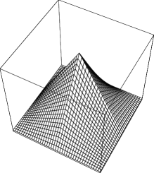
Figure 1: $\varphi_{0}(x,y)$ on its support $[0,2h]^{\times 2}$ with maximum at vertex $(h,h)$.

Motivated by the weak formulation (32), we make the following definition.

Definition 13

Let Assumptions 2 and 11 hold. We call $\psi_{h}:[0,T)\to S_{h}$ with $\psi_{h},\dot{\psi}_{h}\in L^{2}(0,T;S_{h})$ a semidiscrete solution of the Hartree initial boundary-value problem (4) with initial condition $\psi_{0h}\in S_{h}$ if

$$\left\{\begin{array}[]{l}{\rm i}\,\frac{{\rm d}}{{\rm d}t}\,{(\varphi,\psi_{h})}_{L^{2}}={(\nabla\varphi,\nabla\psi_{h})}_{L^{2}}+{(\varphi,v\psi_{h})}_{L^{2}}+{(\varphi,f[\psi_{h}])}_{L^{2}},\quad\forall\varphi\in S_{h},\,\,\forall t\in[0,T),\\ \hskip 34.71234pt\psi_{h}(0)=\psi_{0h}.\end{array}\right.$$ (40)

Remark 14

In general, the weak problem (32) is set up using the Gelfand evolution triple $H_{0}^{1}\subset L^{2}\subset{(H_{0}^{1})}^{\ast}=H^{-1}$. One then looks for weak solutions $\psi\in W_{2}^{1}(0,T;H_{0}^{1},L^{2})\subset C([0,T),L^{2})$ motivating Definition 13.

We assume the Galerkin subspace $S_{h}$ from Assumption 11 to satisfy the following additional approximation and inverse inequalities.

Assumption 15

Let Assumption 11 hold. Then, there exists a constant $C_{A}>0$ s.t.

$$\inf_{\varphi\in S_{h}}\big{(}{\|\psi-\varphi\|}_{L^{2}}+h{\|\psi-\varphi\|}_{H^{1}}\big{)}\leq C_{A}h^{2}{\|\psi\|}_{H^{2}},\quad\forall\psi\in H^{2}\cap H^{1}_{0}.$$

Remark 16

For an order of accuracy $r\geq 2$ of the family $\{S_{h}\}_{h\in(0,1)}$, the usual assumption replaces the r.h.s. by $C_{A}h^{s}{\|\psi\|}_{H^{s}}$ and is asked to hold for all $\psi\in H^{s}\cap H^{1}_{0}$. For simplicity, we stick to Assumption 15.

Assumption 17

Let Assumption 11 hold. Then, there exists a constant $C_{B}>0$ s.t.

$${\|\varphi\|}_{H^{1}}\leq C_{B}h^{-1}{\|\varphi\|}_{L^{2}},\quad\forall\varphi\in S_{h}.$$

Remark 18

For the two-dimensional bilinear Lagrange finite element setting of Remark 12, both Assumption 15 and Assumption 17 hold.

Furthermore, we make an assumption on the approximation quality of the initial condition $\psi_{0h}\in S_{h}$ of the semidiscrete problem (40) compared to the initial condition $\psi_{0}\in H^{2}\cap H^{1}_{0}$ of the continuum problem (7).

Assumption 19

Let Assumption 11 hold. Then, there exists a constant $C_{0}>0$ s.t.

$${\|\psi_{0}-\psi_{0h}\|}_{L^{2}}\leq C_{0}h^{2}.$$ (41)

The semidiscrete scheme has the following conservation properties.

Proposition 20

Let Assumptions 3 and 11 hold, and let $\psi_{h}$ be a semidiscrete solution of the Hartree initial boundary-value problem (4) in the sense of Definition 13. Then, the mass and energy of $\psi_{h}$ are conserved under the time evolution,

$${\mathcal{M}}[\psi_{h}(t)]={\mathcal{M}}[\psi_{0h}],\quad\forall t\in[0,T),$$ (42)

$${\mathcal{H}}[\psi_{h}(t)]={\mathcal{H}}[\psi_{0h}],\quad\forall t\in[0,T).$$

Proof  If we plug $\varphi=\psi_{h}(t)$ into (40) and take the imaginary part of the resulting equation, we get the conservation of the mass. If we plug $\varphi=\dot{\psi}_{h}(t)$ into (40) and take the real part of the resulting equation, we get the conservation of the energy using Assumption 3. $\Box$

Existence-uniqueness is addressed in the following.

Theorem 21

Let Assumptions 3 and 11 hold. Then, there exists a unique global semidiscrete solution $\psi_{h}$ of the Hartree initial-boundary value problem (4) in the sense of Definition 13.

Proof  Let $\{\varphi_{j}\}_{j=1}^{N_{h}}$ be a basis of the Galerkin space $S_{h}$, and let us write

$$\psi_{h}(t)=\sum_{j=1}^{N_{h}}z_{j}(t)\,\varphi_{j}.$$ (43)

Plugging (43) into the semidiscrete system (40), we get for $z(t):=(z_{1}(t),...,z_{N_{h}}(t))\in{\mathord{\mathbb{C}}}^{N_{h}}$,

$$\left\{\begin{array}[]{l}{\rm i}\,\dot{z}(t)=A^{-1}(B+Y)z(t)+A^{-1}H[z(t)]z(t),\quad\forall t\in[0,T),\\ z(0)=z_{0},\end{array}\right.$$ (46)

where $\psi_{0h}=\sum_{j=1}^{N_{h}}(z_{0})_{j}\,\varphi_{j}$ and the matrices $A,B\in{\mathord{\mathbb{C}}}^{N_{h}\times N_{h}}$ are the positive definite mass and stiffness matrices, respectively,

$$A_{ij} := {(\varphi_{i},\varphi_{j})}_{L^{2}},$$

$$B_{ij} := {(\nabla\varphi_{i},\nabla\varphi_{j})}_{L^{2}}.$$

Moreover, $Y\in{\mathord{\mathbb{C}}}^{N_{h}\times N_{h}}$ is the external potential matrix,

$$Y_{ij}:={(\varphi_{i},v\varphi_{j})}_{L^{2}},$$

and the matrix-valued function $H:{\mathord{\mathbb{C}}}^{N_{h}}\to{\mathord{\mathbb{C}}}^{N_{h}\times N_{h}}$ is defined by

$${H[z]}_{ij}:=\sum_{k,l=1}^{N_{h}}\bar{z}_{k}z_{l}\,{(\varphi_{i},\lambda g[\bar{\varphi}_{k}\varphi_{l}]\varphi_{j})}_{L^{2}}.$$

Since the function ${\mathord{\mathbb{C}}}^{N_{h}}\ni z\mapsto A^{-1}(B+Y)z+A^{-1}H[z]z\in{\mathord{\mathbb{C}}}^{N_{h}}$ is locally Lipschitz continuous analogously to the continuum case, the Picard-Lindelöf theory for ordinary differential equations implies local existence and uniqueness of the initial value problem (46). Moreover, this local solution is a global solution if it remains restricted to a compact subset of ${\mathord{\mathbb{C}}}^{N_{h}}$. But this is the case due to the mass conservation from (42). $\Box$

We next turn to the $L^{2}$-error estimate of the semidiscretization. For that purpose, we introduce the Ritz projection.

Definition 22

Let Assumption 11 hold. Then, the Ritz projection $R_{h}:H^{1}_{0}\to S_{h}$ is defined to be the orthogonal projection from $H^{1}_{0}$ onto $S_{h}$ w.r.t. the Dirichlet scalar product ${(\nabla\cdot,\nabla\cdot)}_{L^{2}}$ on $H^{1}_{0}$, i.e.

$${(\nabla\varphi,\nabla R_{h}\psi)}_{L^{2}}={(\nabla\varphi,\nabla\psi)}_{L^{2}},\quad\forall\varphi\in S_{h}.$$ (47)

The Ritz projection satisfies the following error estimate.

Lemma 23

(Cf. [20, p.8]) Let Assumptions 11 and 15 hold. Then, there exists a constant $C_{R}>0$ s.t.

$${\|(1-R_{h})\psi\|}_{L^{2}}+h{\|(1-R_{h})\psi\|}_{H^{1}}\leq C_{R}h^{2}{\|\psi\|}_{H^{2}},\quad\forall\psi\in H^{2}\cap H^{1}_{0}.$$ (48)

The next theorem is the main assertion of this section.

Theorem 24

Let Assumptions 2, 11, 15, and 19 hold, and let $\psi$ be the solution of the continuum problem from Theorem 7 and $\psi_{h}$ the solution of the semidiscrete problem from Theorem 21. Then, for any $0<T<\infty$, there exists a constant $C_{E}>0$ s.t.

$$\max_{t\in[0,T]}{\|\psi(t)-\psi_{h}(t)\|}_{L^{2}}\leq C_{E}h^{2}.$$

Proof  We decompose the difference of $\psi$ and $\psi_{h}$ as

$$\psi(t)-\psi_{h}(t)=\rho(t)+\theta(t),$$

where $\rho(t)$ and $\theta(t)$ are defined with the help of the Ritz projection $R_{h}$ from (47) by

$$\rho(t):=(1-R_{h})\psi(t),\quad\theta(t):=R_{h}\psi(t)-\psi_{h}(t).$$

Making use of the schemes (32), (40), and (47), we can write

$${\rm i}{(\varphi,{\dot{\theta}}(t))}_{L^{2}}-{(\nabla\varphi,\nabla\theta(t))}_{L^{2}} = -{\rm i}{(\varphi,{\dot{\rho}}(t))}_{L^{2}}+{(\varphi,v(\psi(t)-\psi_{h}(t)))}_{L^{2}}$$ (49)

$$+{(\varphi,f[\psi(t)]-f[\psi_{h}(t)])}_{L^{2}}.$$

Plugging $\varphi=\theta(t)\in S_{h}$ into (49) and taking the imaginary part of the resulting equation, we get the differential inequality

$$\frac{1}{2}\,\frac{{\rm d}}{{\rm d}t}\,{\|\theta(t)\|}_{L^{2}}^{2} \leq \left({\|{\dot{\rho}}(t)\|}_{L^{2}}+{\|v(\psi(t)-\psi_{h}(t))\|}_{L^{2}}+{\|f[\psi(t)]-f[\psi_{h}(t)]\|}_{L^{2}}\right){\|\theta(t)\|}_{L^{2}}$$ (50)

$$\leq \left({\|{\dot{\rho}}(t)\|}_{L^{2}}+c_{1}\left({\|\rho(t)\|}_{L^{2}}+{\|\theta(t)\|}_{L^{2}}\right)\right){\|\theta(t)\|}_{L^{2}},$$

where we used the conservation laws (25) and (42) and (23) to define the constant

$$c_{1}:={\|v\|}_{L^{\infty}}+2{\|\lambda\|}_{L^{\infty}}{\|V\|}_{L^{\infty}({\mathord{\mathbb{R}}}^{d})}\left({\mathcal{M}}[\psi_{0}]+{\mathcal{M}}[\psi_{0h}]\right).$$

Using $\epsilon>0$ to regularize the time derivative of ${\|\theta\|}_{L^{2}}$ at $\theta=0$ by rewriting the l.h.s. of (50) as $\frac{1}{2}\frac{{\rm d}}{{\rm d}t}{\|\theta\|}_{L^{2}}^{2}=\frac{1}{2}\frac{{\rm d}}{{\rm d}t}({\|\theta\|}_{L^{2}}^{2}+\epsilon^{2})$, we get

$$\frac{{\rm d}}{{\rm d}t}\left({\|\theta\|}_{L^{2}}^{2}+\epsilon^{2}\right)^{1/2}\leq{\|{\dot{\rho}}(t)\|}_{L^{2}}+c_{1}\left({\|\rho(t)\|}_{L^{2}}+{\|\theta(t)\|}_{L^{2}}\right),$$ (51)

where we used ${\|\theta(t)\|}_{L^{2}}\leq\left({\|\theta\|}_{L^{2}}^{2}+\epsilon^{2}\right)^{1/2}$. Integrating (51) from $0$ to $t$, letting $\epsilon\to 0$, and applying Grönwall’s lemma to the resulting inequality, we find

$${\|\theta(t)\|}_{L^{2}} \leq {\|\theta(0)\|}_{L^{2}}+\int_{0}^{t}\!{\rm d}s\,\big{(}{\|{\dot{\rho}}(s)\|}_{L^{2}}+c_{1}{\|\rho(s)\|}_{L^{2}}\big{)}$$ (52)

$$+\,c_{1}\int_{0}^{t}\!{\rm d}s\,\Big{(}{\|\theta(0)\|}_{L^{2}}+\int_{0}^{s}\!{\rm d}u\,\big{(}{\|{\dot{\rho}}(u)\|}_{L^{2}}+c_{1}{\|\rho(u)\|}_{L^{2}}\big{)}\Big{)}\,{\rm e}^{c_{1}(t-s)}.$$

In order to extract the factor $h^{2}$, we apply (48) and Assumption 19 to get

$${\|\rho(t)\|}_{L^{2}} \leq C_{R}{\|\psi(t)\|}_{H^{2}}h^{2},$$ (53)

$${\|{\dot{\rho}}(t)\|}_{L^{2}} \leq C_{R}{\|{\dot{\psi}}(t)\|}_{H^{2}}h^{2},$$ (54)

$${\|\theta(0)\|}_{L^{2}} \leq \big{(}C_{0}+C_{R}{\|\psi_{0}\|}_{H^{2}}\big{)}h^{2}.$$ (55)

Plugging (53), (54), and (55) into (52), we finally arrive at

$${\|\psi(t)-\psi_{h}(t)\|}_{L^{2}}\leq{\|\theta(t)\|}_{L^{2}}+{\|\rho(t)\|}_{L^{2}}\leq c_{2}(t)h^{2},$$

where the time dependent prefactor is defined by

$$c_{2}(t) := \big{(}C_{0}+C_{R}{\|\psi_{0}\|}_{H^{2}}\big{)}{\rm e}^{c_{1}t}+C_{R}\int_{0}^{t}\!{\rm d}s\,\big{(}{\|{\dot{\psi}}(s)\|}_{H^{2}}+c_{1}{\|\psi(s)\|}_{H^{2}}\big{)}$$

$$+c_{1}C_{R}\int_{0}^{t}\!{\rm d}s\int_{0}^{s}\!{\rm d}u\,\big{(}{\|{\dot{\psi}}(u)\|}_{H^{2}}+c_{1}{\|\psi(u)\|}_{H^{2}}\big{)}\,{\rm e}^{c_{1}(t-s)}+C_{R}{\|\psi(t)\|}_{H^{2}}.$$

Setting $C_{E}:=\max_{t\in[0,T]}c_{2}(t)$ brings the proof of Theorem 24 to an end. $\Box$

Remark 25

For the local case $f[\psi]=|\psi|^{2}\psi$, one replaces the original locally Lipschitz nonlinearity $f$ by a globally Lipschitz continuous nonlinearity which coincides with $f$ in a given neighborhood of the solution $\psi$ of the continuum problem. One then first shows that the semidiscrete solution of the modified problem satisfies the desired $L^{2}$-error bound, and, second, that for $h$ sufficiently small, the modified solution lies in the given neighborhood of $\psi$. But for such $h$, the solution of the modified problem coincides with the solution of the original problem, and, hence, the solution of the original problem satisfies the desired $L^{2}$-error bound, too.

4 The fully discrete approximation

In this section, we discretize the semidiscrete problem (40) in time. To this end, let us denote by $N\in{\mathord{\mathbb{N}}}$ the desired fineness of the time discretization with time discretization scale $\tau$ and its multiples $t_{n}$ for all $n=0,1,2,...,N$,

$$\tau:=\frac{T}{N},\quad t_{n}:=n\tau.$$ (56)

As mentioned in the Introduction, we will use two different time discretization schemes of Crank-Nicholson type to approximate the semidiscrete solution $\psi_{h}$ of Theorem 21 at time $t_{n}$ by $\Psi_{n}\in\Psi$, where

$$\Psi:=(\Psi_{0},\Psi_{1},...,\Psi_{N})\in S_{h}^{\times(N{+}1)}.$$ (57)

These two schemes differ in the way of approximating the nonlinear term $g_{V}[|\psi|^{2}]\psi$ as follows. Let ${\mathcal{N}}:=\{1,2,...,N\}$ and ${\mathcal{N}}_{0}:={\mathcal{N}}\cup\{0\}$, and define

$$\Psi_{n-1/2}:=\frac{1}{2}\left(\Psi_{n}+\Psi_{n-1}\right),\quad\forall n\in{\mathcal{N}}.$$ (58)

Then, the first scheme implements the one-step one-stage Gauss-Legendre Runge-Kutta method in which the nonlinear term is discretized by

$$g_{V}[|\Psi_{n-1/2}|^{2}]\Psi_{n-1/2}.$$ (59)

In this method, the mass ${\mathcal{M}}[\Psi_{n}]$ is conserved under the discrete time evolution. The second scheme, introduced in [9] and applied in [1], discretizes the nonlinear term by

$$g_{V}[\tfrac{1}{2}(|\Psi_{n}|^{2}+|\Psi_{n-1}|^{2})]\Psi_{n-1/2}.$$ (60)

This method, in addition to the mass, also conserves the energy ${\mathcal{H}}[\Psi_{n}]$ of the system. In the following, for convenience, we will call the first scheme coherent and the second one incoherent.

Coherent scheme

In order to define what we mean by a coherent solution of the Hartree initial-boundary value problem (4), we define

$${\dot{\Psi}}_{n}:=\frac{1}{\tau}\left(\Psi_{n}-\Psi_{n-1}\right),\quad\forall n\in{\mathcal{N}}.$$

Definition 26

Let Assumption 2 and 11 hold. We call $\Psi\in S_{h}^{\times(N{+}1)}$ a coherent fully discrete solution of the Hartree initial-boundary value problem (4) with initial condition $\psi_{0h}\in S_{h}$ if

$$\left\{\begin{array}[]{l}{\rm i}{(\varphi,{\dot{\Psi}}_{n})}_{L^{2}}={(\nabla\varphi,\nabla\Psi_{n-1/2})}_{L^{2}}+\,{(\varphi,v\Psi_{n-1/2})}_{L^{2}}+{(\varphi,f[\Psi_{n-1/2}])}_{L^{2}},\\ \hskip 71.13188pt\forall\varphi\in S_{h},\,\forall n\in{\mathcal{N}},\\ \Psi_{0}=\psi_{0h}.\end{array}\right.$$ (64)

The coherent solution has the following conservation property.

Proposition 27

Let $\Psi\in S_{h}^{\times(N{+}1)}$ be a coherent fully discrete solution of the Hartree initial-boundary value problem (4) in the sense of Definition 26. Then, the mass of $\Psi$ is conserved under the discrete time evolution,

$${\mathcal{M}}[\Psi_{n}]={\mathcal{M}}[\psi_{0h}],\quad\forall n\in{\mathcal{N}}_{0}.$$ (65)

Proof  If we plug $\varphi=\Psi_{n-1/2}$ into (64) and take the imaginary part of the resulting equation, we get

$$0={\rm Im}\,{\rm i}{(\Psi_{n-1/2},{\dot{\Psi}}_{n})}_{L^{2}}=\frac{1}{2\tau}\left({\mathcal{M}}[\Psi_{n}]-{\mathcal{M}}[\Psi_{n-1}]\right).$$

$\Box$

Remark 28

The energy ${\mathcal{H}}[\Psi_{n}]$ of the coherent solution (64) is not conserved under the discrete time evolution, see [1] and references therein, in particular [17] and [21] for the local case with $d=1$.

The question of existence and uniqueness of a coherent solution is addressed in the following.

Theorem 29

Let Assumptions 2, 11, and 17 hold, and let the time discretization scale $\tau$ be sufficiently small. Then, there exists a unique coherent fully discrete solution of the Hartree initial-boundary value problem (4) in the sense of Definition 26.

Proof  Let $\phi\in S_{h}$ be given, and define the mapping $F_{\phi}:S_{h}\to S_{h}$ by

$${(\varphi,F_{\phi}[\psi])}_{L^{2}}:={(\varphi,\phi)}_{L^{2}}-\frac{{\rm i}\tau}{2}\,\big{(}{(\nabla\varphi,\nabla\psi)}_{L^{2}}+{(\varphi,v\psi)}_{L^{2}}+{(\varphi,f[\psi])}_{L^{2}}\big{)},\quad\forall\varphi\in S_{h}.$$ (66)

For some $n\in{\mathcal{N}}$, let the $n$-th component $\Psi_{n-1}$ of $\Psi\in S_{h}^{\times(N{+}1)}$ from (57) be given. Adding $2{\rm i}\,(\varphi,\Psi_{n-1})/\tau$ on both sides of (64), we can rewrite (64) with the help of (66) in the form of a fixed point equation for $\Psi_{n-1/2}$,

$$\Psi_{n-1/2}=F_{\Psi_{n-1}}[\Psi_{n-1/2}],$$ (67)

from which we retrieve the unknown component $\Psi_{n}$ by (58). In order to construct the unique solution of (67), we make use of Banach’s fixed point theorem on the compact ball ${\mathcal{B}}_{n-1}:=\{\psi\in S_{h}\,|\,{\|\psi\|}_{L^{2}}\leq{\mathcal{M}}[\Psi_{n-1}]^{1/2}+1\}$ in $S_{h}$. Using Assumption 17 and (23), we get, for $\psi,\xi\in S_{h}$,

$$|{(\varphi,F_{\Psi_{n-1}}[\psi]-F_{\Psi_{n-1}}[\xi])}_{L^{2}}|$$ (68)

$$\leq\frac{\tau}{2}\Big{(}C_{B}^{2}h^{-2}+{\|v\|}_{L^{\infty}}+2{\|\lambda\|}_{L^{\infty}}{\|V\|}_{L^{\infty}({\mathord{\mathbb{R}}}^{d})}\big{(}{\|\psi\|}_{L^{2}}^{2}+{\|\xi\|}_{L^{2}}^{2}\big{)}\Big{)}{\|\psi-\xi\|}_{L^{2}}{\|\varphi\|}_{L^{2}}.$$

Plugging $\varphi=F_{\Psi_{n-1}}[\psi]-F_{\Psi_{n-1}}[\xi]$ into (68) and picking $\psi$ and $\xi$ from ${\mathcal{B}}_{n-1}$, we find

$${\|F_{\Psi_{n-1}}[\psi]-F_{\Psi_{n-1}}[\xi]\|}_{L^{2}}\leq\frac{\alpha_{n-1}}{2}\,\tau{\|\psi-\xi\|}_{L^{2}},$$ (69)

where the constant $\alpha_{n-1}$ is defined, for all $n\in{\mathcal{N}}$, by

$$\alpha_{n-1}:=C_{B}^{2}h^{-2}+{\|v\|}_{L^{\infty}}+4{\|\lambda\|}_{L^{\infty}}{\|V\|}_{L^{\infty}({\mathord{\mathbb{R}}}^{d})}({\mathcal{M}}[\Psi_{n-1}]^{1/2}+1)^{2}.$$ (70)

Let now $\alpha_{n-1}({\mathcal{M}}[\Psi_{n-1}]^{1/2}+1)\tau\leq 1$. Then, it follows from (69) and (70) that $F_{\Psi_{n-1}}$ maps ${\mathcal{B}}_{n-1}$ into ${\mathcal{B}}_{n-1}$ (set $\xi=0$ in (69)) and that $F_{\Psi_{n-1}}$ is a strict contraction on ${\mathcal{B}}_{n-1}$. Therefore, for such $\tau$, Banach’s fixed point theorem implies the existence of a unique solution $\Psi_{n-1/2}\in{\mathcal{B}}_{n-1}$ of the fixed point equation (67). Moreover, due to the mass conservation (65), there exists no solution $\Psi_{n-1/2}$ of (67) with $\Psi_{n-1/2}\in S_{h}\setminus{\mathcal{B}}_{n-1}$. Hence, the component $\Psi_{n}$ of the coherent solution exists and is unique for such $\tau$. Starting at $\Psi_{0}=\psi_{0h}$ and proceeding iteratively, we get all $n+1$ components of the coherent solution $\Psi\in S_{h}^{\times(N{+}1)}$. Moreover, again due to (65), we get a uniform bound on the size of the time discretization scale $\tau$, e.g.

$$\alpha_{0}({\mathcal{M}}[\psi_{0h}]^{1/2}+1)\tau\leq 1.$$

$\Box$

Remark 30

Since $\alpha_{0}\geq C_{B}^{2}h^{-2}$, we have that $\tau\leq C_{B}^{-2}h^{2}$, where $C_{B}$ stems from Assumption 17.

We next turn to the first of the two main assertions of the present paper which is the time quadratic accuracy estimate on the $L^{2}$-error of the coherent solution.

Theorem 31

Let Assumptions 2, 11, 15, and 19 hold, and let $\Psi\in S_{h}^{\times(N{+}1)}$ be the coherent solution from Theorem 29. Then, there exists a constant $C_{K}>0$ s.t.

$$\max_{n\in{\mathcal{N}}_{0}}{\|\psi(t_{n})-\Psi_{n}\|}_{L^{2}}\leq C_{K}(\tau^{2}+h^{2}).$$

Remark 32

The constant $C_{K}$ depends on higher Sobolev norms of the continuum solution $\psi$. These norms exist due to the regularity assertion in Theorem 7 (c).

Proof  Let $n\in{\mathcal{N}}$ be fixed and define $\psi_{n}:=\psi(t_{n})$ with $t_{n}$ from (56). As in the proof of Theorem 24, we decompose the difference to be estimated as

$$\psi_{n}-\Psi_{n}=\rho_{n}+\theta_{n},$$ (71)

where $\rho_{n}$ and $\theta_{n}$ are again defined with the help of the Ritz projection from (47) by

$$\rho_{n}:=(1-R_{h})\psi_{n},\quad\theta_{n}:=R_{h}\psi_{n}-\Psi_{n}.$$ (72)

Using Taylor’s theorem in order to expand $\psi_{n}$ around $t=0$ up to zeroth order in $t_{n}$ and the estimate on the Ritz projection (48), we immediately get

$${\|\rho_{n}\|}_{L^{2}}\leq C_{R}h^{2}\Big{(}{\|\psi_{0}\|}_{H^{2}}+\int_{0}^{t_{n}}\!\!{\rm d}t\,\,{\|{\dot{\psi}}(t)\|}_{H^{2}}\Big{)}.$$ (73)

In order to estimate $\theta_{n}$, we want to extract suitable small differences from the expression

$$L_{n,\varphi}:=\frac{{\rm i}}{\tau}{(\varphi,\theta_{n}-\theta_{n-1})}_{L^{2}}-\frac{1}{2}{(\nabla\varphi,\nabla(\theta_{n}+\theta_{n-1}))}_{L^{2}}-\frac{1}{2}{(\varphi,v(\theta_{n}+\theta_{n-1}))}_{L^{2}}$$ (74)

which contains all the linear terms in (64) moved to the l.h.s. with $\Psi_{n}$ replaced by $\theta_{n}$. For this purpose, we first plug the definition of $\theta_{n}$ into (74), and then use the definition of the Ritz projection (47) and the scheme (64) to get

$$L_{n,\varphi} = \frac{{\rm i}}{\tau}\,{(\varphi,R_{h}(\psi_{n}-\psi_{n-1}))}_{L^{2}}-\frac{1}{2}{(\nabla\varphi,\nabla(\psi_{n}+\psi_{n-1}))}_{L^{2}}-\frac{1}{2}{(\varphi,vR_{h}(\psi_{n}+\psi_{n-1}))}_{L^{2}}$$ (75)

$$-\,{(\varphi,f[\Psi_{n-1/2}])}_{L^{2}}.$$

Rewriting the first term on the r.h.s. of (75) with the help of the continuum solution satisfying the weak formulation (32), we have

$$\frac{{\rm i}}{\tau}\,{(\varphi,R_{h}(\psi_{n}-\psi_{n-1}))}_{L^{2}} = \frac{{\rm i}}{\tau}\,{(\varphi,(R_{h}-1)(\psi_{n}-\psi_{n-1}))}_{L^{2}}+{\rm i}\,{(\varphi,\tfrac{1}{\tau}(\psi_{n}-\psi_{n-1})-{\dot{\psi}}_{n-1/2})}_{L^{2}}$$ (76)

$$+\,{(\nabla\varphi,\nabla\psi_{n-1/2})}_{L^{2}}+{(\varphi,v\psi_{n-1/2})}_{L^{2}}+{(\varphi,f[\psi_{n-1/2}])}_{L^{2}},$$

where we used the notations $\psi_{n-1/2}:=\psi(t_{n}-\tau/2)$ and ${\dot{\psi}}_{n-1/2}:={\dot{\psi}}(t_{n}-\tau/2)$. Plugging (76) into (75), we can express $L_{n,\varphi}$ in the form

$$L_{n,\varphi}=\sum_{j=1}^{6}\,{(\varphi,\omega_{n}^{(j)})}_{L^{2}},$$ (77)

where the functions $\omega_{n}^{(j)}$ with $j=1,...,6$ are defined by

$$\omega_{n}^{(1)} := \frac{{\rm i}}{\tau}(R_{h}-1)(\psi_{n}-\psi_{n-1}),$$

$$\omega_{n}^{(2)} := {\rm i}\big{(}\tfrac{1}{\tau}(\psi_{n}-\psi_{n-1})-{\dot{\psi}}_{n-1/2}\big{)},$$

$$\omega_{n}^{(3)} := \Delta\big{(}\tfrac{1}{2}\left(\psi_{n}+\psi_{n-1}\big{)}-\psi_{n-1/2}\right),$$

$$\omega_{n}^{(4)} := v\left(\psi_{n-1/2}-\tfrac{1}{2}\left(\psi_{n}+\psi_{n-1}\right)\right),$$

$$\omega_{n}^{(5)} := \frac{1}{2}\,v\left(1-R_{h}\right)\left(\psi_{n}+\psi_{n-1}\right),$$

$$\omega_{n}^{(6)} = f[\psi_{n-1/2}]-f[\Psi_{n-1/2}],$$

and, for $\omega_{n}^{(3)}$, we used again ${(\nabla\varphi,\nabla\psi)}_{L^{2}}={(\varphi,-\Delta\psi)}_{L^{2}}$ for all $\psi\in H^{2}\cap H^{1}_{0}$. Plugging $\varphi=(\theta_{n}+\theta_{n-1})/2$ into (74) and (77), and taking the imaginary part of the resulting equation, we get

$${\|\theta_{n}\|}_{L^{2}}\leq{\|\theta_{n-1}\|}_{L^{2}}+\tau\sum_{j=1}^{6}{\|\omega_{n}^{(j)}\|}_{L^{2}}.$$ (78)

Let us next estimate the terms ${\|\omega_{n}^{(j)}\|}_{L^{2}}$ for all $j=1,...,6$. For $\omega_{n}^{(1)}$, we expand $\psi_{n}$ around $t=t_{n-1}$ up to zeroth order in $\tau$ and use (48) s.t.

$${\|\omega_{n}^{(1)}\|}_{L^{2}}\leq{C_{R}h^{2}}\tau^{-1}\int_{t_{n-1}}^{t_{n}}\!\!{\rm d}t\,\,{\|{\dot{\psi}}(t)\|}_{H^{2}}.$$ (79)

For $\omega_{n}^{(2)}$, we expand $\psi_{n-1}$ and $\psi_{n}$ around $t=t_{n}-\tau/2$ up to second order in $\tau/2$,

$${\|\omega_{n}^{(2)}\|}_{L^{2}} \leq \frac{1}{2\tau}\Big{(}\int_{t_{n-1}}^{t_{n}-\tau/2}\!\!{\rm d}t\,\,(t_{n-1}-t)^{2}{\|{\dddot{\psi}}(t)\|}_{L^{2}}+\int_{t_{n}-\tau/2}^{t_{n}}\!\!{\rm d}t\,\,(t_{n}-t)^{2}{\|{\dddot{\psi}}(t)\|}_{L^{2}}\Big{)}$$ (80)

$$\leq \frac{\tau}{8}\int_{t_{n-1}}^{t_{n}}\!\!{\rm d}t\,\,{\|{\dddot{\psi}}(t)\|}_{L^{2}}.$$

Analogously, for $\omega_{n}^{(3)}$ and $\omega_{n}^{(4)}$, we expand $\psi_{n-1}$ and $\psi_{n}$ around $t=t_{n}-\tau/2$ up to first order in $\tau/2$,

$${\|\omega_{n}^{(3)}\|}_{L^{2}} \leq \frac{\tau}{4}\int_{t_{n-1}}^{t_{n}}\!\!{\rm d}t\,\,{\|\Delta{\ddot{\psi}}(t)\|}_{L^{2}},$$ (81)

$${\|\omega_{n}^{(4)}\|}_{L^{2}} \leq \frac{\tau}{4}\,{\|v\|}_{L^{\infty}}\int_{t_{n-1}}^{t_{n}}\!\!{\rm d}t\,\,{\|{\ddot{\psi}}(t)\|}_{L^{2}}.$$ (82)

For $\omega_{n}^{(5)}$, expanding $\psi_{n-1}$ and $\psi_{n}$ around $t=0$ up to zeroth order in time, we get, analogously to the estimate of $\omega_{n}^{(1)}$,

$${\|\omega_{n}^{(5)}\|}_{L^{2}}\leq C_{R}h^{2}{\|v\|}_{L^{\infty}}\Big{(}{\|\psi_{0}\|}_{H^{2}}+\int_{0}^{t_{n}}\!\!{\rm d}t\,\,{\|{\dot{\psi}}(t)\|}_{H^{2}}\Big{)}.$$ (83)

Finally, for $\omega_{n}^{(6)}$, we apply the local Lipschitz continuity (23) to get

$${\|\omega_{n}^{(6)}\|}_{L^{2}}\leq c_{1}\,{\|\psi_{n-1/2}-\Psi_{n-1/2}\|}_{L^{2}},$$ (84)

where we used the continuum mass conservation (25) and the coherent fully discrete mass conservation (65) to define the constant

$$c_{1}:=2{\|\lambda\|}_{L^{\infty}}{\|V\|}_{L^{\infty}({\mathord{\mathbb{R}}}^{d})}\left({\mathcal{M}}[\psi_{0}]+{\mathcal{M}}[\psi_{0h}]\right).$$ (85)

Since we want to reinsert the decomposition (71) into the r.h.s. of (84), we write

$${\|\psi_{n-1/2}-\Psi_{n-1/2}\|}_{L^{2}} \leq {\|\psi_{n-1/2}-\tfrac{1}{2}(\psi_{n}+\psi_{n-1})\|}_{L^{2}}$$ (86)

$$+\,\frac{1}{2}\left({\|\rho_{n-1}\|}_{L^{2}}+{\|\rho_{n}\|}_{L^{2}}+{\|\theta_{n-1}\|}_{L^{2}}+{\|\theta_{n}\|}_{L^{2}}\right).$$

Plugging the estimates (73), (79) to (84), and (86) into (78), we find

$${\|\theta_{n}\|}_{L^{2}}{\leq\|\theta_{n-1}\|}_{L^{2}}+\big{(}A^{(1)}_{n}+\tau A^{(2)}_{n}\big{)}h^{2}+A^{(3)}_{n}\tau^{2}+\frac{c_{1}}{2}\,\tau\left({\|\theta_{n-1}\|}_{L^{2}}+{\|\theta_{n}\|}_{L^{2}}\right),$$ (87)

where the first term on the r.h.s. of (86) was estimated as in $\omega_{n}^{(3)}$ or $\omega_{n}^{(4)}$, and

$$A^{(1)}_{n} := C_{R}\int_{t_{n-1}}^{t_{n}}\!\!{\rm d}t\,\,{\|\dot{\psi}(t)\|}_{H^{2}},$$ (88)

$$A^{(2)}_{n} := C_{R}\left(c_{1}+{\|v\|}_{L^{\infty}}\right)\Big{(}{\|\psi_{0}\|}_{H^{2}}+\int_{0}^{t_{n}}\!\!{\rm d}t\,\,{\|\dot{\psi}(t)\|}_{H^{2}}\Big{)},$$ (89)

$$A^{(3)}_{n} := \frac{1}{4}\left(c_{1}+{\|v\|}_{L^{\infty}}\right)\int_{t_{n-1}}^{t_{n}}\!\!{\rm d}t\,\,{\|\ddot{\psi}(t)\|}_{L^{2}}+\frac{1}{8}\int_{t_{n-1}}^{t_{n}}\!\!{\rm d}t\,\,{\|\dddot{\psi}(t)\|}_{L^{2}}+\,\frac{1}{4}\int_{t_{n-1}}^{t_{n}}\!\!{\rm d}t\,\,{\|\Delta\ddot{\psi}(t)\|}_{L^{2}}.\quad$$ (90)

If we choose the time discretization scale $\tau$ to be small enough, e.g. $c_{1}\tau\leq 1$, we can construct the following recursive bound on ${\|\theta_{n}\|}_{L^{2}}$ from inequality (87),

$${\|\theta_{n}\|}_{L^{2}}\leq B^{(1)}{\|\theta_{n-1}\|}_{L^{2}}+B^{(2)}_{n},$$ (91)

where we used that $1/(1-c_{1}\tau/2)\leq 1+c_{1}\tau$ if $c_{1}\tau\leq 1$ to define

$$B^{(1)} := (1+c_{1}\tau)^{2},$$

$$B^{(2)}_{n} := (1+c_{1}\tau)\big{(}\!\big{(}A^{(1)}_{n}+\tau A^{(2)}_{n}\big{)}h^{2}+A^{(3)}_{n}\tau^{2}\big{)}.$$

Therefore, if we iterate the bound (91) until we arrive at ${\|\theta_{0}\|}_{L^{2}}$, we get

$${\|\theta_{n}\|}_{L^{2}} \leq \left(B^{(1)}\right)^{n}{\|\theta_{0}\|}_{L^{2}}+\sum_{k=1}^{n}\left(B^{(1)}\right)^{n-k}B^{(2)}_{k}$$ (92)

$$\leq c_{2}\Big{(}{\|\theta_{0}\|}_{L^{2}}+\sum_{k=1}^{n}\big{(}\big{(}A^{(1)}_{k}+\tau A^{(2)}_{k}\big{)}h^{2}+A^{(3)}_{k}\tau^{2}\big{)}\Big{)},$$

where, on the second line of (92), we first extract the global factor $(B^{(1)})^{n}$ which can then be estimated as $(B^{(1)})^{n}\leq(1+c_{1}T/N)^{2N}\leq c_{2}$ with the definition

$$c_{2}:={\rm e}^{2c_{1}T}.$$ (93)

It remains to estimate ${\|\theta_{0}\|}_{L^{2}}$ on the r.h.s. of (92). This is again done by using the estimate on the Ritz projection (48),

$${\|\theta_{0}\|}_{L^{2}} \leq {\|\psi_{0}-\psi_{0h}\|}_{L^{2}}+{\|(R_{h}-1)\psi_{0}\|}_{L^{2}}$$ (94)

$$\leq {\|\psi_{0}-\psi_{0h}\|}_{L^{2}}+C_{R}h^{2}{\|\psi_{0}\|}_{H^{2}}.$$

Hence, with estimate (73) on ${\|\rho_{n}\|}_{L^{2}}$ and the estimates (92) and (94) on ${\|\theta_{n}\|}_{L^{2}}$ in the decomposition (72), taking the maximum over all times, we finally arrive at

$$\max_{n\in{\mathcal{N}}_{0}}{\|\psi_{n}-\Psi_{n}\|}_{L^{2}}\leq c_{2}{\|\psi_{0}-\psi_{0h}\|}_{L^{2}}+c_{3}h^{2}+c_{4}\tau^{2},$$ (95)

where the constants $c_{3}$ and $c_{4}$ are defined by

$$c_{3} := C_{R}\left(1+c_{2}\left(1+T\left(c_{1}+{\|v\|}_{L^{\infty}}\right)\right)\right)\Big{(}{\|\psi_{0}\|}_{H^{2}}+\int_{0}^{T}\!\!{\rm d}t\,\,{\|\dot{\psi}(t)\|}_{H^{2}}\Big{)},$$ (96)

$$c_{4} := \frac{c_{2}}{4}\,\Big{(}(c_{1}+{\|v\|}_{L^{\infty}})\int_{0}^{T}\!\!{\rm d}t\,\,{\|\ddot{\psi}(t)\|}_{L^{2}}+\frac{1}{2}\int_{0}^{T}\!\!{\rm d}t\,\,{\|\dddot{\psi}(t)\|}_{L^{2}}+\int_{0}^{T}\!\!{\rm d}t\,\,{\|\Delta\ddot{\psi}(t)\|}_{L^{2}}\Big{)}.$$ (97)

The constants $c_{1}$ and $c_{2}$ are given in (85) and (93), respectively. Using Assumption 19 and setting $C_{K}:=\max\{c_{2}C_{0}+c_{3},c_{4}\}$ brings the proof of Theorem 31 to an end. $\Box$

Remark 33

We can compute an explicit bound on the integrands in (96) and (97) on any finite time interval. As an example, for the last term in the constant $c_{4}$ from (97), we have

$${\|\Delta\ddot{\psi}(t)\|}_{L^{2}}\leq{\|\Delta^{3}\psi(t)\|}_{L^{2}}+{\|\Delta^{2}J[\psi(t)]\|}_{L^{2}}+{\|\Delta\tfrac{{\rm d}}{{\rm d}t}J[\psi(t)]\|}_{L^{2}}.$$

The first term is exponentially bounded in time using the conditions from Theorem 7 (a) and (b) and Grönwall’s lemma on the Duhamel integral form of the differential equation (7),

$${\|\Delta^{3}\psi(t)\|}_{L^{2}}\leq{\|\Delta^{3}\psi_{0}\|}_{L^{2}}\,{\rm e}^{C({\mathcal{M}}[\psi_{0}])t},$$

where the constant $C$ stems from (21). The second term is again bounded due to (10). Finally, the third term is bounded due to equation (24) for the time derivative of the nonlinear term $J[\psi(t)]$ and the corresponding estimates (19) and (20).

Incoherent scheme

As described at the beginning of Section 4, we also study a second discretization scheme which approximizes the nonlinear term $g_{V}[|\psi|^{2}]\psi$ not by (59) but rather by the expression (60).

Definition 34

Let Assumptions 2 and 11 hold. We call $\Psi\in S_{h}^{\times(N+1)}$ an incoherent fully discrete solution of the Hartree initial-boundary value problem (4) with initial condition $\psi_{0h}\in S_{h}$ if

$$\left\{\begin{array}[]{l}{\rm i}\,{(\varphi,\dot{\Psi}_{n})}_{L^{2}}={(\nabla\varphi,\nabla\Psi_{n-1/2})}_{L^{2}}+{(\varphi,v\Psi_{n-1/2})}_{L^{2}}+{(\varphi,\tfrac{1}{2}\lambda g_{V}[|\Psi_{n}|^{2}+|\Psi_{n-1}|^{2}]\Psi_{n-1/2})}_{L^{2}},\\ \hskip 71.13188pt\forall\varphi\in S_{h},\,\,\forall n\in{\mathcal{N}},\\ \Psi_{0}=\psi_{0h}.\end{array}\right.$$ (101)

The incoherent solution has the following conservation properties.

Proposition 35

Let $\Psi\in S_{h}^{\times(N+1)}$ be an incoherent fully discrete solution of the Hartree initial-boundary value problem (4) in the sense of Definition 34, and let Assumption 3 hold. Then, the mass and the energy of $\Psi$ are conserved under the discrete time evolution,

$${\mathcal{M}}[\Psi_{n}] = {\mathcal{M}}[\psi_{0h}],\quad\forall n\in{\mathcal{N}}_{0},$$ (102)

$${\mathcal{H}}[\Psi_{n}] = {\mathcal{H}}[\psi_{0h}],\quad\forall n\in{\mathcal{N}}_{0}.$$

Proof  Plugging $\varphi=\Psi_{n-1/2}$ into (101) and taking the imaginary part of the resulting equation leads to the mass conservation as in the proof of Proposition 27. In order to prove the energy conservation, we plug $\varphi=\dot{\Psi}_{n}$ into (101) and take the real part of the resulting equation. Using that ${(\Psi_{n},\lambda g_{V}[|\Psi_{n-1}|^{2}]\Psi_{n})}_{L^{2}}={(\Psi_{n-1},\lambda g_{V}[|\Psi_{n}|^{2}]\Psi_{n-1})}_{L^{2}}$ due to Assumption 3, we get

$$0={\rm Re}\,\,{\rm i}{(\dot{\Psi}_{n},\dot{\Psi}_{n})}_{L^{2}}=\frac{1}{2\tau}\left({\mathcal{H}}[\Psi_{n}]-{\mathcal{H}}[\Psi_{n-1}]\right).$$

$\Box$

We next turn to the proof of existence-uniqueness of the incoherent solution.

Theorem 36

Let Assumptions 2, 11, and 17 hold, and let the time discretization scale $\tau$ be sufficiently small. Then, there exists a unique incoherent fully discrete solution of the Hartree initial- boundary value problem (4) in the sense of Definition 34.

Proof  The proof for the incoherent solution is analogous to the proof of the coherent solution. Let $\phi\in S_{h}$ be given, and define the mapping $G_{\phi}:S_{h}\to S_{h}$ by

$${(\varphi,G_{\phi}[\psi])}_{L^{2}} := {(\varphi,\phi)}_{L^{2}}$$ (103)

$$-\frac{{\rm i}\tau}{2}\left({(\nabla\varphi,\nabla\psi)}_{L^{2}}+{(\varphi,v\psi)}_{L^{2}}+{(\varphi,\tfrac{1}{2}\lambda g_{V}[|2\psi-\phi|^{2}+|\phi|^{2}]\psi)}_{L^{2}}\right),\quad\forall\varphi\in S_{h}.$$

For some $n\in{\mathcal{N}}$, let the $n$-th component $\Psi_{n-1}$ of $\Psi\in S_{h}^{\times(N+1)}$ from (57) be given. Adding $2{\rm i}(\varphi,\Psi_{n-1})/\tau$ on both sides of (101), we rewrite (101) with the help of (103) in the form of a fixed point equation for $\Psi_{n-1/2}$,

$$\Psi_{n-1/2}=G_{\Psi_{n-1}}[\Psi_{n-1/2}].$$

In order to make use of Banach’s fixed point theorem as in the proof of Theorem 29, we show that $G_{\Psi_{n-1}}$ maps the compact Ball ${\mathcal{B}}_{n-1}:=\{\psi\in S_{h}\,|\,{\|\psi\|}_{L^{2}}\leq{\mathcal{M}}[\Psi_{n-1}]^{1/2}+1\}$ into itself and that $G_{\Psi_{n-1}}$ is a strict contraction on ${\mathcal{B}}_{n-1}$. To this end, we write

$$|{(\varphi,G_{\Psi_{n-1}}[\psi]-G_{\Psi_{n-1}}[\xi])}_{L^{2}}|$$ (104)

$$\leq\frac{\tau}{2}\Big{(}{\|\nabla(\psi-\xi)\|}_{L^{2}}{\|\nabla\varphi\|}_{L^{2}}+{\|v\|}_{L^{\infty}}{\|\psi-\xi\|}_{L^{2}}{\|\varphi\|}_{L^{2}}+\,\frac{1}{2}\,A{\|\varphi\|}_{L^{2}}\Big{)},$$

where, with the help of (16), (22), and $||z|^{2}-|w|^{2}|\leq|z+w||z-w|$ for all $z,w\in{\mathord{\mathbb{C}}}$, the third term $A$ on the r.h.s. of (104) can be estimated as

$$A := {\|\lambda g_{V}[|2\psi-\Psi_{n-1}|^{2}+|\Psi_{n-1}|^{2}]\psi-\lambda g_{V}[|2\xi-\Psi_{n-1}|^{2}+|\Psi_{n-1}|^{2}]\xi\|}_{L^{2}}$$

$$\leq 8{\|\lambda\|}_{L^{\infty}}{\|V\|}_{L^{\infty}({\mathord{\mathbb{R}}}^{d})}\,\big{(}{\|\psi\|}_{L^{2}}^{2}+{\|\xi\|}_{L^{2}}^{2}+{\|\Psi_{n-1}\|}_{L^{2}}^{2}\big{)}{\|\psi-\xi\|}_{L^{2}}.$$

Hence, plugging $\varphi=G_{\Psi_{n-1}}[\psi]-G_{\Psi_{n-1}}[\xi]$ into (104), we get for $\psi,\xi\in{\mathcal{B}}_{n-1}$ using Assumption 17,

$${\|G_{\Psi_{n-1}}[\psi]-G_{\Psi_{n-1}}[\xi]\|}_{L^{2}}\leq\frac{\alpha_{n-1}}{2}\,\tau\,{\|\psi-\xi\|}_{L^{2}},$$

where $\alpha_{n-1}:=C_{B}^{2}h^{-2}+{\|v\|}_{L^{\infty}}+12{\|\lambda\|}_{L^{\infty}}{\|V\|}_{L^{\infty}({\mathord{\mathbb{R}}}^{d})}\,({\mathcal{M}}[\Psi_{n-1}]^{1/2}+1)^{2}$ like in the coherent scheme (70). Therefore, we arrive at the claim as in the proof of Proposition 29 using the mass conservation from (102), i.e. the incoherent solution exists and is unique if the time discretization scale $\tau$ is sufficiently small, e.g. $\alpha_{0}({\mathcal{M}}[\psi_{0h}]^{1/2}+1)\tau\leq 1$. $\Box$

Finally, we also provide a time quadratic accuracy estimate on the $L^{2}$-error of the incoherent solution. Again, the proof is analogous to the corresponding proof for the coherent solution from Theorem 31.

Theorem 37

Let Assumptions 2, 11, 15, and 19 hold, and let $\Psi\in S_{h}^{\times(N{+}1)}$ be the incoherent solution from Theorem 36. Then, there exists a constant $C_{I}>0$ s.t.

$$\max_{n\in{\mathcal{N}}_{0}}{\|\psi(t_{n})-\Psi_{n}\|}_{L^{2}}\leq C_{I}(\tau^{2}+h^{2}).$$

Proof  As in (71) and (72), we make use of the decomposition $\psi_{n}-\Psi_{n}=\rho_{n}+\theta_{n}$, and we estimate $\rho_{n}$ again by (73). In order to estimate ${\|\theta_{n}\|}_{L^{2}}$, we define $L_{n,\varphi}$ as in (74). Then, everything in equation (75) remains unchanged up to the last term which is replaced by the expression $-(\varphi,\tfrac{1}{2}\lambda g_{V}[|\Psi_{n}|^{2}+|\Psi_{n-1}|^{2}]\Psi_{n-1/2})$. Using again (76), we can rewrite $L_{n,\varphi}$ as in equation (77), where the terms $\omega_{n}^{(j)}$ remain unchanged for all $j=1,...,5$, whereas the term $\omega_{n}^{(6)}$ now has the form

$$\omega_{n}^{(6)} := f[\psi_{n-1/2}]-\lambda g_{V}[\tfrac{1}{2}(|\Psi_{n}|^{2}+|\Psi_{n-1}|^{2})]\Psi_{n-1/2}$$

$$= \omega_{n,1}^{(6)}+\omega_{n,2}^{(6)}+\omega_{n,3}^{(6)},$$

where we use the same notation as introduced after (76) to define

$$\omega_{n,1}^{(6)} := \lambda g_{V}[|\psi_{n-1/2}|^{2}](\psi_{n-1/2}-\tfrac{1}{2}(\psi_{n}+\psi_{n-1})),$$

$$\omega_{n,2}^{(6)} := \frac{1}{2}\,\lambda g_{V}[|\psi_{n-1/2}|^{2}-\tfrac{1}{2}(|\psi_{n}|^{2}+|\psi_{n-1}|^{2})](\psi_{n}+\psi_{n-1}),$$

$$\omega_{n,3}^{(6)} := \frac{1}{2}\,\lambda g_{V}[\tfrac{1}{2}(|\psi_{n}|^{2}+|\psi_{n-1}|^{2})](\psi_{n}+\psi_{n-1})-\lambda g_{V}[\tfrac{1}{2}(|\Psi_{n}|^{2}+|\Psi_{n-1}|^{2})]\Psi_{n-1/2}.$$

For $\omega_{n,1}^{(6)}$, expanding $\psi_{n-1}$ and $\psi_{n}$ around $t=t_{n}-\tau/2$ up to first order in $\tau/2$, we get , using (16) and the mass conservation (25),

$${\|\omega_{n,1}^{(6)}\|}_{L^{2}}\leq\frac{\tau}{4}\,{\|\lambda\|}_{L^{\infty}}{\|V\|}_{L^{\infty}({\mathord{\mathbb{R}}}^{d})}{\mathcal{M}}[\psi_{0}]\int_{t_{n-1}}^{t_{n}}\!{\rm d}t\,\,{\|\ddot{\psi}(t)\|}_{L^{2}}.$$ (105)

In order to estimate $\omega_{n,2}^{(6)}$, we expand $\psi_{n-1}$ and $\psi_{n}$ around $t=t_{n}-\tau/2$ up to first order in $\tau/2$ and get similarly

$${\|\omega_{n,2}^{(6)}\|}_{L^{2}} \leq {\|\lambda\|}_{L^{\infty}}{\|V\|}_{L^{\infty}({\mathord{\mathbb{R}}}^{d})}{\mathcal{M}}[\psi_{0}]^{1/2}{\||\psi_{n-1/2}|^{2}-\tfrac{1}{2}(|\psi_{n}|^{2}+|\psi_{n-1}|^{2})\|}_{L^{1}}$$ (106)

$$\leq a^{(0)}(a_{n}^{(1)}\tau+a_{n}^{(2)}\tau^{2}+a_{n}^{(3)}\tau^{3}),$$

where we define

$$a^{(0)} := {\|\lambda\|}_{L^{\infty}}{\|V\|}_{L^{\infty}({\mathord{\mathbb{R}}}^{d})}{\mathcal{M}}[\psi_{0}]^{1/2},$$

$$a_{n}^{(1)} := {\mathcal{M}}[\psi_{0}]\int_{t_{n-1}}^{t_{n}}\!{\rm d}t\,\,{\|\ddot{\psi}(t)\|}_{L^{2}}$$

$$a_{n}^{(2)} := \frac{1}{2}\,{\|\dot{\psi}_{n-1/2}\|}_{L^{2}}\Big{(}{\|\dot{\psi}_{n-1/2}\|}_{L^{2}}+\int_{t_{n-1}}^{t_{n}}\!{\rm d}t\,\,{\|\ddot{\psi}(t)\|}_{L^{2}}\Big{)}$$

$$a_{n}^{(3)} := \frac{1}{8}\int_{t_{n-1}}^{t_{n}}\!{\rm d}t\,\,{\|\ddot{\psi}(t)\|}_{L^{2}}^{2}.$$

For $\omega_{n,3}^{(6)}$, using in particular again $||z|^{2}-|w|^{2}|\leq|z+w||z-w|$ for all $z,w\in{\mathord{\mathbb{C}}}$ and the decomposition (71), we get

$${\|\omega_{n,3}^{(6)}\|}_{L^{2}} \leq \frac{1}{4}\,{\|\lambda g_{V}[|\psi_{n}|^{2}+|\psi_{n-1}|^{2}](\psi_{n}-\Psi_{n}+\psi_{n-1}-\Psi_{n-1})\|}_{L^{2}}$$ (107)

$$+\frac{1}{4}\,{\|\lambda g_{V}[|\psi_{n}|^{2}-|\Psi_{n}|^{2}+|\psi_{n-1}|^{2}-|\Psi_{n-1}|^{2}](\Psi_{n}+\Psi_{n-1})\|}_{L^{2}}$$

$$\leq {\|\lambda\|}_{L^{\infty}}{\|V\|}_{L^{\infty}({\mathord{\mathbb{R}}}^{d})}({\mathcal{M}}[\psi_{0}]+{\mathcal{M}}[\psi_{0h}])(\|\rho_{n}\|+\|\rho_{n-1}\|+\|\theta_{n}\|+\|\theta_{n-1}\|).$$

Therefore, plugging the estimates (105), (106), and (107) into (78), we again find the closed inequality (87), the coefficients $A_{n}^{(1)}$ and $A_{n}^{(2)}$ having the same form as in (88) and (89), respectively. Using estimate (105) on $\omega_{n,1}^{(6)}$, we see that the coefficient $A_{n}^{(3)}$ in the incoherent case contains all the terms from (90) of the coherent case with $c_{1}$ replaced by $a^{(0)}$, plus an additional term of the form $a^{(0)}(a_{n}^{(1)}+a_{n}^{(2)}\tau+a_{n}^{(3)}\tau^{2})$ which is due to the estimate (106) of $\omega_{n,2}^{(6)}$. Plugging the coefficients $A_{n}^{(1)}$, $A_{n}^{(2)}$, and $A_{n}^{(3)}$ into the iterated bound (92) and using estimate (94) on $\theta_{0}$, we again get an estimate of the form (95) where the constant $c_{3}$ has the same form as in (96) whereas the constant $c_{4}$, compared to (97), now looks like

$$c_{4} := \frac{c_{2}}{4}\Big{(}(a^{(0)}+{\|v\|}_{L^{\infty}})\int_{0}^{T}\!\!{\rm d}t\,\,{\|\ddot{\psi}(t)\|}_{L^{2}}+\frac{1}{2}\int_{0}^{T}\!\!{\rm d}t\,\,{\|\dddot{\psi}(t)\|}_{L^{2}}+\int_{0}^{T}\!\!{\rm d}t\,\,{\|\Delta\ddot{\psi}(t)\|}_{L^{2}}\Big{)}$$ (108)

$$+c_{2}a^{(0)}\big{(}{\mathcal{M}}[\psi_{0}]+\tfrac{1}{2}\,T\max_{t\in[0,T]}{\|\dot{\psi}(t)\|}_{L^{2}}\big{)}\int_{0}^{T}\!\!{\rm d}t\,\,{\|\ddot{\psi}(t)\|}_{L^{2}}$$

$$+\frac{c_{2}a^{(0)}}{2}T\max_{t\in[0,T]}{\|\dot{\psi}(t)\|}_{L^{2}}^{2}+\frac{c_{2}a^{(0)}}{8}T^{2}\int_{0}^{T}\!\!{\rm d}t\,\,{\|\ddot{\psi}(t)\|}_{L^{2}}^{2}.$$

Herewith, as in the proof of Theorem 31, we arrive at the assertion. $\Box$

Remark 38

Using estimates as in Remark 33, we can again bound the constants in (108) explicitly.

References

- [1] Akrivis G D, Dougalis V A, and Karakashian O A 1991 On fully discrete Galerkin methods of second-order temporal accuracy for the nonlinear Schrödinger equation Numer. Math. 59 31–53
- [2] Aschbacher W H 2001 Large systems of non-relativistic Bosons and the Hartree equation Diss. ETH No. 14135
- [3] Aschbacher W H, in progress
- [4] Aschbacher W H, Fröhlich J, Graf G M, Schnee K, and Troyer M 2002 Symmetry breaking regime in the nonlinear Hartree equation J. Math. Phys. 43 3879–91
- [5] Aschbacher W H and Squassina M 2008 On phase segregation in nonlocal two-particle Hartree systems, submitted, and arXiv:0809.3369
- [6] Brenner S C and Scott L R 1994 The mathematical theory of finite element methods (New York: Springer)
- [7] Brezis H and Gallouet T 1980 Nonlinear Schrödinger evolution equations Nonlinear Anal. 4 677–81
- [8] Caliari M and Squassina M 2008 Location and phase segregation of ground and excited states for 2D Gross-Pitaevskii systems Dyn. Partial Differential Equations 5 117–37
- [9] Delfour M, Fortin M, and Payre G 1981 Finite-difference solutions of a non-linear Schrödinger equation J. Comput. Phys. 44 277–88
- [10] Elgart A, Erdös L, Schlein B, and Yau H T 2004 Nonlinear Hartree equation as the mean field limit of weakly coupled fermions J. Math. Pures Appl. 83, 1241–73
- [11] Erdös L, Schlein B, and Yau H T 2007 Rigorous derivation of the Gross-Pitaevskii equation Phys. Rev. Lett. 98 040404
- [12] Fröhlich J, Tsai T P, and Yau H T 2000 On a classical limit of quantum theory and the nonlinear Hartree equation Geom. funct. anal. 57–78
- [13] Fröhlich J, Gustafson S, Jonsson B L G, and Sigal I M 2004 Solitary wave dynamics in an external potential Commun. Math. Phys. 250 613–42
- [14] Lieb E, Seiringer R, and Yngvason J 2000 Bosons in a trap: a rigorous derivation of the Gross-Pitaevskii energy functional Phys. Rev. A 61 043602
- [15] Onorato M, Osborne A R, and Serio M 2006 Modulational instability in crossing sea states: a possible mechanism for the formation of freak waves Phys. Rev. Lett 96 014503
- [16] Reed M and Simon B 1975 Methods of modern mathematical physics II (New York: Academic Press)
- [17] Sanz-Serna J M and Verwer J G 1986 Conservative and nonconservative schemes for the solution of the nonlinear Schrödinger equation IMA J. Numer. Anal. 6 25–42
- [18] Shukla P K, Kourakis I, Eliasson B, Marklund M, and Stenflo L 2006 Instability and evolution of nonlinearly interacting water waves Phys. Rev. Lett. 97 094501
- [19] Spohn H 1980 Kinetic equations from Hamiltonian dynamics Rev. Mod. Phys. 52 569–615
- [20] Thomée V 1997 Galerkin finite element methods for parabolic problems Springer Series in Computational Mathematics, Vol. 25 (Berlin: Springer)
- [21] Tourigny Y and Morris J Ll 1988 An investigation into the effect of product approximation in the numerical solution of the cubic nonlinear Schrödinger equation J. Comput. Phys. 76 103–30
- [22] Zeidler E 1990 Nonlinear functional analysis and its applications II/A (New York: Springer)