Nonlocal Gluon Condensate from the Dyson–Schwinger Equations

Abstract

We establish a novel method of obtaining the gauge-invariant bilocal condensate of gluon fields from the solutions of the Dyson–Schwinger equations (DSE) which works in the infrared and ultraviolet limits. We present explicit results for $SU(3)$ case in four dimensions, and compare to other related analytical and lattice results.

Motivation: The non-perturbative QCD vacuum is known for the presence of gluon (and quark) condensates Shifman et al. (1979). These objects are in general studied in a local approximation. A bilocal object can be introduced by using operator product expansion (OPE) Mikhailov (1993). However, OPE method can work only at a short scale. The infrared (IR) behaviour of gluon condensate is of importance because it acts as a potential in which quarks fluctuate Lavelle and Schaden (1988). Therefore, to understand, e.g. how QCD vacuum properties are modified in the infrared by external electromagnetic fields Rafelski (1998), one must first understand the dynamics of the gauge field condensate and than quark condensate in a scheme operational in the infrared.

We obtain here the gauge-invariant nonlocal condensate in terms of perturbative and non-perturbative propagators. Then we solve numerically the Dyson–Schwinger equations (DSE) for $SU(3)$ gauge theory at approximately two loops, following the methods developed by Bloch Bloch (2003) and other authors to obtain the non-perturbative propagators. We introduce perturbative propagators in a way which is consistent with the non-perturbative ones, and extract the gauge field condensate. Finally we analyze the condensate dependence on distance, and compare with prior results obtained by analytical and lattice methods.

Form factors and nonlocal condensate: We start with the $SU(N_{c}=3)$ gauge field action

$$S=-\frac{1}{4}\frac{\mathrm{tr}}{N_{c}}\int d^{4}xG_{\mu\nu}G^{\mu\nu},$$ (1)

where $G_{\mu\nu}=G_{\mu\nu}^{a}T^{a}$, $G_{\mu\nu}^{a}=\partial_{\mu}A_{\nu}^{a}-\partial_{\nu}A_{\mu}^{a}+gf^{abc}A_{\mu}^{b}A_{\nu}^{c}$, $\mathrm{tr}T^{a}T^{b}=N_{c}\delta^{ab}$. The gluon propagator $D_{F\mu\nu}^{ab}$ is considered in Landau gauge $D_{F\mu\nu}^{ab}(x)=-i\langle T\left(A_{\mu}^{a}(x)A_{\nu}^{b}(0)\right)\rangle$ with a form factor $F(p^{2})$

$$D_{F\mu\nu}^{ab}(p)=\delta^{ab}\left(g_{\mu\nu}-\frac{p_{\mu}p_{\nu}}{p^{2}}\right)\frac{F(p^{2})}{p^{2}+i\epsilon},$$ (2)

and the ghost propagator is defined as $D^{Gab}(x)=-i\langle T\left(c^{a}(x)c^{b}(0)\right)\rangle$, with the ghost form factor $G(p^{2})$,

$$D^{Gab}(p)=\frac{\delta^{ab}}{p^{2}+i\epsilon}G(p^{2}).$$ (3)

Following Ref. Dosch and Simonov (1988), the bilocal condensate is defined as the vacuum expectation value (VEV) of the following gauge-invariant operator

$$\mathcal{F}(y-z)=\langle:\frac{\alpha}{\pi}\frac{\mathrm{tr}}{N_{c}}\left[G_{\mu\nu}(y)W(y,z)G^{\mu\nu}(z)W(z,y)\right]:\rangle,$$ (4)

where Wilson–Polyakov lines are $W(y,z)=\mathcal{P}\mathrm{exp}\left(ig\int^{z}_{y}A_{\mu}dx^{\mu}\right)$, $\mathcal{P}$ being the path-ordering symbol. Note that the normal ordering in Eq. (4) is defined with respect to the perturbative (PT) vacuum, whereas the operators are averaged over a non-perturbative (NP) vacuum.

We are going to work at below the two-loop limit, thus Eq. (4) is expanded perturbatively up to $\alpha^{2}$-order:

$$\mathcal{F}=\mathcal{F}^{(0)}+\mathcal{F}^{(1)}_{1}+\mathcal{F}^{(1)}_{2}+\mathcal{F}^{(1)}_{3}$$ (5)

indices ${}^{(0)},^{(1)}$ denoting $\alpha$ order. The two-gluon piece is

$$\mathcal{F}^{(0)}=\langle:\frac{\alpha}{\pi}\frac{\mathrm{tr}}{N_{c}}\left[G^{\mathrm{Lin}\mu\nu}(x)G^{\mathrm{Lin}}_{\mu\nu}(0)\right]:\rangle,$$ (6)

where we have split the gauge covariant quantity $G_{\mu\nu}$ into a linear (Abelian) and a bilinear non-gauge covariant objects $G^{\mathrm{Lin}}_{\mu\nu}=G_{\mu\nu}+ig[A_{\mu},A_{\nu}].$ Three-gluon term is absent, and a four-gluon term without Wilson lines is

$$\mathcal{F}^{(1)}_{1}=\langle:\frac{\alpha}{\pi}\frac{\mathrm{tr}}{N_{c}}\left\{g[A_{\mu}(x),A_{\nu}(x)]g[A_{\mu}(0),A_{\nu}(0)]\right\}:\rangle.$$ (7)

Wilson lines do not non-trivially contribute to the above $\mathcal{F}^{(0)}$ and $\mathcal{F}^{(1)}_{1}$, but contribute to $\mathcal{F}^{(1)}_{2}$ and $\mathcal{F}^{(1)}_{3}$:

$$\begin{array}[]{rcl}\displaystyle\mathcal{F}^{(1)}_{2}(x)\!&\!\displaystyle=\!&\!\displaystyle\langle:\frac{\alpha}{\pi}\frac{\mathrm{tr}}{N_{c}}\left[\int\!\!\!\!\int g^{2}F_{\mu\nu}(x)A_{\beta}\left(u(\tau)\right)A_{\gamma}\left(v(\sigma)\right)\times\right.\\ \displaystyle\hfil&\times&\displaystyle F^{\mu\nu}(0)\dot{u}^{\beta}\dot{v}^{\gamma}\theta(\tau-\sigma)d\tau d\sigma\bigg{]}:\rangle,\\ \displaystyle\mathcal{F}^{(1)}_{3}\!&\!\displaystyle=\!&\!\displaystyle\langle:\frac{\alpha}{\pi}\frac{\mathrm{tr}}{N_{c}}\left[\int\!\!\!\!\int g^{2}F_{\mu\nu}(x)A_{\beta}\left(u(\tau)\right)\times\right.\\ &\times&\displaystyle F^{\mu\nu}(0)A_{\gamma}\left(v(\sigma)\right)\dot{v}^{\gamma}\dot{u}^{\beta}d\tau d\sigma\bigg{]}:\rangle\end{array}$$ (8)

We use here straight lines $v^{\gamma}(\sigma)=\sigma x^{\gamma},u^{\beta}(\tau)=\tau x^{\beta},$ running over $\tau\in(0,1),\sigma\in(0,1)$.

To express $\mathcal{F}^{(0)},\mathcal{F}^{(1)}_{1,2,3}$ in terms of propagators, we need to handle the PT-normal products in the NP-vacuum. Consider an operator $\mathcal{O}(x)$. A $T$-product of operators can be evaluated in both perturbative and non-perturbative vacuum, with $G^{PT,NP}_{\mathcal{O}}$ defined as follows:

$$\begin{array}[]{rcl}T\left(\mathcal{O}(x)\mathcal{O}(y)\right)&=&:\mathcal{O}(x)\mathcal{O}(y):^{PT}+iG^{PT}_{\mathcal{O}}(x,y)=\\[5.69046pt] &=&:\mathcal{O}(x)\mathcal{O}(y):^{NP}+iG^{NP}_{\mathcal{O}}(x,y),\end{array}$$ (9)

indices $NP$ and $PT$ over normal ordering symbols and Green’s functions meaning the definitions of the latter in the nonperturbative or perturbative vacuum correspondingly. Taking a VEV over the nonperturbative vacuum, and subtracting the $NP$ definition of $T\left[\mathcal{O}(x)\mathcal{O}(y)\right]$ from the $PT$ one, one sees that

$$\langle:\mathcal{O}(x)\mathcal{O}(y):^{PT}\rangle_{NP}=i(G^{NP}_{\mathcal{O}}(x,y)-G^{PT}_{\mathcal{O}}(x,y)).$$ (10)

Thus emerges the object of interest

$$\Delta_{F}(p^{2})\equiv\alpha(p^{2})\left(F^{NP}(p^{2})-F^{PT}(p^{2})\right).$$ (11)

In our case the non-perturbative form factor $F^{NP}(p^{2})=F(p^{2})$, Eq. (2), is what we obtain from solving the DSE. The corresponding perturbative form factor $F^{PT}(p^{2})$ is discussed below. For the sake of generality we present, using Eq. (6), the components of condensates in an arbitrary dimension $d$:

$$\mathcal{F}^{(0)}=2(d-1)d_{c}\int\frac{d^{d}p}{(2\pi)^{d}}\Delta_{F}(p^{2})e^{ipx},$$ (12)

in agreement with Ref. Namyslowski , where a local limit of this equation is given, here and below $d_{c}=N_{c}^{2}-1$. For the subleading terms we obtain:

$$\mathcal{F}^{(1)}_{1}=4d_{c}N_{c}\left[(d^{2}-2d-1)I_{1}^{2}-I_{2\mu\nu}I_{2}^{\mu\nu}\right],$$ (13)

where the propagator moments are defined as

$$\begin{array}[]{rcl}I_{1}(x)&=&\int\frac{d^{d}p}{(2\pi)^{d}}\frac{\Delta_{F}(p^{2})}{p^{2}}e^{ipx}\\[5.69046pt] I_{2\mu\nu}(x)&=&\int\frac{d^{d}p}{(2\pi)^{d}}\frac{\Delta_{F}(p^{2})}{p^{2}}\frac{p_{\mu}p_{\nu}}{p^{2}}e^{ipx}.\end{array}$$ (14)

For the terms containing Wilson lines, one has

$$\mathcal{F}^{(1)}_{2}+\mathcal{F}^{(1)}_{3}=4d_{c}N_{c}W_{1}W_{2},$$ (15)

the moments $W_{1},W_{2}$ being

$$W_{1}\! = \int\frac{d^{d}p}{(2\pi)^{4}}\Delta_{F}(p^{2})e^{ipx},$$ (16)

$$W_{2}\! = \!12(1-d)\!\int\!\!\frac{d^{d}p}{(2\pi)^{d}}\frac{\Delta_{F}(p^{2})}{p^{2}}\!\left(x^{2}\!-\frac{(px)^{2}}{p^{2}}\right)\!\frac{\sin^{2}\left(\frac{px}{2}\right)}{(px)^{2}}.$$

To be able to complete the evaluation of the nonlocal condensate we should supply the non-perturbative and perturbative form factors into these equations.

Dyson–Schwinger equations: To obtain the needed non-perturbative input form factor $F^{NP}(p^{2})$ one option is to solve DSE. We work in pure gluodynamics, following closely Bloch’s method Bloch (2003) of IR analysis and his truncation labeled (A.1), Table 3 ibid., thus we do not give here the full details. The procedure of writing down, truncating, IR-analyzing and solving DSE is developed and described in detail in many works, see for example Hauck et al. (1998); Fischer and Alkofer (2003); Fischer (2008); Fischer et al. (2008); Alkofer et al. (2008). The DSE equations in a covariant gauge are organized in the following way:

$$\left\{\begin{array}[]{l}\frac{1}{G(p^{2})}-\frac{1}{G(\sigma_{g}^{2})}=-\left(\Sigma(p^{2})-\Sigma(\sigma_{g}^{2})\right)\\[5.69046pt] \frac{1}{F(p^{2})}-\frac{1}{F(\sigma_{f}^{2})}=-\left(\Pi(p^{2})-\Pi(\sigma_{f}^{2})\right),\end{array}\right.$$ (17)

where $\sigma_{g}$ and $\sigma_{c}$ are renormalization points for gluon and ghost propagator respectively. After truncation, the ghost self-energy and the gluon vacuum polarization are,

$$\begin{array}[]{rcl}\Sigma(p^{2})&=&N_{c}g_{\mu}^{2}\int T_{0}(p^{2},q^{2},r^{2})G(q^{2})F(r^{2})\frac{d^{d}q}{(2\pi)^{d}},\\[5.69046pt] \Pi(p^{2})&=&\Pi^{2c}(p^{2})+\Pi^{2g}(p^{2})+\Pi^{4g}(p^{2})\end{array}$$ (18)

where $g_{\mu}=\sqrt{4\pi\alpha(\mu)}$, $\mu$ is renormalization point, and separate contributions to vacuum polarization are

$$\begin{array}[]{rcl}\displaystyle\Pi^{2c}(p^{2})&=&\int\frac{d^{d}q}{(2\pi)^{d}}M_{0}(p^{2},q^{2},r^{2})G(q^{2})G(r^{2}),\\[5.69046pt] \Pi^{2g}(p^{2})&=&\int\frac{d^{d}q}{(2\pi)^{4}}Q_{0}(p^{2},q^{2},r^{2})G(q^{2})G(r^{2}),\\[5.69046pt] \Pi^{4g}(p^{2})&=&\int\frac{d^{d}q}{(2\pi)^{d}}Q_{4}(p^{2},q^{2},r^{2})\times\\ &&\times G(q^{2})^{3}F(q^{2})^{3/4}G(r^{2})F(r^{2})^{1/4},\end{array}$$ (19)

with kernels $M_{0},Q_{0},Q_{4},T_{0}$ defined in Bloch (2003), eqs. (47, 48, 49, E.1). Here $x=p^{2},y=q^{2},z=r^{2}$, $r^{2}=(p-q)^{2}$.

We decompose the gluon and ghost form factors in a set of Chebyshev polynomials $T_{i}(z)$ on an interval $p^{2}\in(\epsilon,\sigma)$, and use a power-like Ansatz for the IR domain $p^{2}\in(0,\epsilon)$:

$$F(z)=\left\{\begin{array}[]{l}\exp{\left(\sum_{i}f_{i}T_{i}(z)\right)},z>\epsilon\\[8.5359pt] Az^{2\kappa},z<\epsilon\end{array}\right.,$$ (20)

and a similar decomposition is assumed for $G$, where $z=\log\frac{p^{2}}{\mu_{0}^{2}}$, $\mu_{0}$ is scale unit, continuity is imposed at $p^{2}=\epsilon$, renormalization points are chosen for gluon and ghost respectively, $\sigma_{f}=\sigma,\sigma_{g}=0$, normalization conditions $F(\sigma)=1$, $1/G(0)=0$; and from now on, $d=4$. For the two sets of coefficients we get algebraic equations, which are solved by Newton’s method. Reliability of the method is supported by convergence of the sets of coefficients.

Choice of scale: Upon solving the equations, we construct running coupling out of the form factors from DSE

$$\alpha(p^{2})=\alpha(\mu)F(p^{2})G^{2}(p^{2}).$$ (21)

This follows since we did not include the ghost-ghost-gluon vertex factor into the system of DSE, it is considered to be unity. Here $\mu$ is the renormalization scale for coupling, which is identical with the ultraviolet  (UV) cutoff in our case: $\mu=\sigma$, and $F(\mu^{2})=G(\mu^{2})=1$

To relate the gauge coupling constant $\alpha$ with physics, one must introduce a scale. Physical scale is not fully defined in this problem, for we cannot actually compare pure gluodynamics to real-world QCD with fermions. Even so, we note that any object of dimension $k$ must be measured in units of $\mu_{0}^{k}$, where scale $\mu_{0}$ is one and the same for the whole problem. By comparing our (non-perturbative) $\alpha$ with the standard running coupling value Amsler et al. (2008) we obtain a rough estimate for our scale $\mu_{0}$

$$\alpha(\sqrt{s}=10\mathrm{GeV})=0.18,\,\,\to\mu_{0}\sim 0.55\mathrm{GeV}.$$ (22)

For comparison, an estimate performed at $\sqrt{s}=m_{\tau}=1.77\mathrm{GeV},\,\,\alpha=0.35$ yields $\mu_{0}=0.8$.

From DSE to condensates: Our solutions of DSE confirm the results by Bloch in every feature; thus we proceed to applying them for obtaining the condensate. The form factors which we have obtained and the running coupling are true non-perturbative quantities $F^{NP}(z),G^{NP}(z),\alpha(z)$. Now, in order to employ Eq. (4), we need the difference between the perturbative and non-perturbative objects.

Bloch in Bloch (2003) observes that he reproduced the leading-order PT results for coupling in the UV, but not the NLO. We confirm this by comparison of $\beta(\alpha)$ and anomalous dimension $\gamma(\alpha)$ for the propagator, see below, with their perturbative behaviour. We believe this is a consequence of the partial rather than full resummation of the perturbation series, since not all of the NLO diagrams emergent from the systematic expansion appear in DSE as solved here, due to the truncation of the hierarchy of DSE. In this sense we might call the present approximation resummed 1.5 loops. Resummed, since the partial resummation extends to all orders. For possible improvements of our method, it would be advantageous to use DSE with vertex function included Alkofer et al. (2008).

Given that the DSE solution is of infinite order in $\alpha$, but incomplete as of 2nd order, one must re-evaluate perturbation theory form factor, rendering it consistent with the partial resummation inherent in the truncated DSE. This must be always done since DSE is always in practical work a truncated system. Gluon form factor, normalized at $\mu$, is expected to be organized in the form:

$$F(p^{2})=\exp\left(\int_{\alpha(\mu^{2})}^{\alpha(p^{2})}\frac{b(\alpha)}{\alpha}d\alpha\right),$$ (23)

where $b(\alpha(z))=\alpha(z)\gamma(\alpha(z))/\beta(\alpha(z))$, $z$, as before, is renormgroup time. Functions $\beta(\alpha)$ and $\gamma(\alpha)$ are nonperturbative and given by:

$$\beta(\alpha(z))=\frac{\partial\alpha(z)}{\partial z},\qquad\gamma(\alpha(z))=\frac{\partial\log F(z)}{\partial z}.$$ (24)

In perturbation theory Larin and Vermaseren (1993) $b^{PT}(\alpha)=\frac{1}{\alpha}\sum_{i=0}b_{i}\alpha^{i}$, where $b_{0}^{PT}=\frac{13}{22},\,b_{1}^{PT}=\frac{537}{968},b_{2}^{PT}=\left(\frac{129791}{42592}-\frac{243\zeta(3)}{176}\right)$. However instead of these $b_{i}^{PT}$ we must use results of a polynomial fit in the UV range of our ratio $b(\alpha)=\frac{\alpha\gamma(\alpha)}{\beta(\alpha)}$:

$$b(\alpha)\stackrel{{\scriptstyle\mathrm{Fit}}}{{\to}}\sum_{i=0}^{n}\tilde{b}_{i}\alpha^{i}(z)=\tilde{b}^{PT}(\alpha).$$ (25)

To obtain a reasonable precision, $n=2$ suffices. Using $\beta,\gamma$ from DSE and having performed the fit Eq. (25), we apply the coefficients $\tilde{b}_{i}$ to build an “effective” perturbative expression for gluon form factor, which is to be afterwards subtracted from the NP expression:

$$F^{PT}(p^{2})=\exp\left(\int_{\alpha(\mu^{2})}^{\alpha(p^{2})}\frac{1}{\alpha}\sum_{i=0}\tilde{b}_{i}\alpha^{i}d\alpha\right).$$ (26)

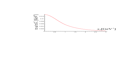
Figure 1: The nonlocal gluon condensate in $3+1$-dimensional $SU(3)$ from DSE approach, scale fixed at 10 GeV.

We have now got both, a non-perturbative propagator from solving DSE, and the perturbative propagator, Eq. (26). Thus we can obtain the nonlocal condensate shown in figure 1. This is our main computational result. Our solution qualitatively satisfies the expectations which are due to the known UV and IR forms of the condensate, prescribed by OPE and lattice respectively. OPE predicts at small distances Mikhailov (1993)

$$\mathcal{F}(x)=G_{0}^{2}(1-\lambda^{2}x^{2}).$$ (27)

Comparison with this short-distance behaviour is shown in table 1. At large distances one can use  Di Giacomo et al. (2002)

$$\mathcal{F}(x)=Ce^{-ax},$$ (28)

(to be used with caution, as some other predictions e.g. from instanton models Dorokhov et al. (2000), exist). It is instructive to inspect numerical convergence to the values of $G_{0}^{2},\lambda^{2},C,a$ shown in table 2, as function of the number $n$ of polynomials involved. Results are stated for scale fixed at 10 GeV. The remaining numerical error in the determination of the magnitude of condensate and correlation lengths can be eliminated by increasing the size of the basis, once there is merit in such an effort. Bloch Bloch (2003) used $n=50$ in solving DSE. We estimate our current numerical error based on convergence shown in table 2 and show this in the bottom entries in table 1.

Conclusion: We described here what we believe is a novel idea allowing to obtain the non perturbative vacuum condensate, which has the capability of yielding both IR and UV vacuum properties. This approach is less expensive than lattice simulations, and more universal than OPE.

Table 1: Comparison our results with prior work. “SR” denotes sum rules, $\tau$ means “$\tau$ decay”. Results of our present Letter given in bold in the two last lines, denoted by $\dagger$ and $\ddagger$, for scale fixing points 1.8 GeV and 10 GeV respectively. Error bars are given in parentheses.

Method	Yr.	Ref.	$G_{0}^{2}$[$\mathrm{GeV}^{4}$]	$\lambda^{2}$[$\mathrm{GeV}^{2}]$	$C[\mathrm{GeV}^{4}]$	$a[\mathrm{GeV}$]
SR	’78	Shifman et al. (1979)	.012	–	–	.–
OPE	’92	Mikhailov (1993)	–	.21	–	–
Lattice	’97	D’Elia et al. (1997)	.015	–	.008	.6
Lattice	’02	D’Elia et al. (2003)	–	–	.08	.8
SR	’02	Ioffe (2003)	.009(.007)	–	–	–
$\tau$	’02	Ioffe (2003)	.006(.012)	–	–	–
DSE	’08	$\dagger$	.062(.022)	2.3(.6)	.09(.03)	1.9(.4)
DSE	’08	$\ddagger$	.014(.005)	1.1(.3)	.020(.007)	1.3(.3)

Table 2: Convergence of condensates and correlation lengths with respect to the number of polynomials $n$.

$n$	$G_{0}^{2}$[$\mathrm{GeV}^{4}$]	$\lambda^{2}$[$\mathrm{GeV}^{2}$]	$C[\mathrm{GeV}^{4}]$	$a[\mathrm{GeV}]$
22	0.00834	1.04052	0.02671	2.26331
24	0.01068	0.64805	0.01854	1.22284
26	0.00967	1.30711	0.01573	1.41736
28	0.01270	1.18162	0.01892	1.33049
30	0.01352	1.12676	0.01977	1.28204

Our main result is the demonstration that the solution of DSE allows determination of the full nonlocal gluon condensate $\langle:\frac{\alpha}{\pi}\frac{\mathrm{tr}}{N_{c}}G_{\mu\nu}(x)W(x,0)G_{\mu\nu}(0)W(0,x):\rangle$ as a function of coordinate or momentum. From these one can get its fundamental properties: the value at zero separation and correlation range. Our results are obtained in Landau gauge, yet the procedure and thus the final answer are gauge-invariant. Our here presented method and results suggest that the effort required, especially including Fermi (quark) fields, is greatly reduced compared to lattice method.

Moreover, in principle there seems to be no obstacle to the study of the far infrared limit, which relies of further development of DSE in this domain. Our pure gauge theory results cannot be as yet used for further phenomenological developments due to scale uncertainty; however, the purpose of this paper was to demonstrate in principle how an a priori calculation of condensate is possible in the framework of DSE.

Acknowledgements: We are grateful to Jacques Bloch for introducing us into the details of his DSE method. We thank A. Bakulev, A. Dorokhov and S. Mikhailov for discussions. Numerical calculations were performed in part on the Computational Cluster of the Theoretical Division of INR RAS, Moscow. A.Z. would like to thank D.V. Shirkov and A.S. Gorsky for their kind advice. We thank P.D. Dr. Peter Thirolf and Prof. Dr. D. Habs, Director of the Cluster of Excellence in Laser Physics – Munich-Center for Advanced Photonics (MAP) for their hospitality in Garching while much of this research was carried out. This research was supported in part by RFBR Grant 07-01-00526, by the DFG–LMUexcellent grant, and by a grant from: the U.S. Department of Energy DE-FG02-04ER4131.

References

- Shifman et al. (1979) M. A. Shifman, A. I. Vainshtein, and V. I. Zakharov, Nucl. Phys. B147, 385 (1979).
- Mikhailov (1993) S. V. Mikhailov, Phys. Atom. Nucl. 56, 650 (1993).
- Lavelle and Schaden (1988) M. J. Lavelle and M. Schaden, Phys. Lett. B208, 297 (1988).
- Rafelski (1998) J. Rafelski in Frontier Tests of QED and Physics of the Vacuum, E. Zavattini et al eds., (Heron Press, Sofia 1998) pp 425-439; and Quantum Chromodynamics Paris, France 1–6 June 1998, World Scientific, H. Fried and B. Muller, eds., pp 208-223, eprint hep-ph/9806389.
- Bloch (2003) J. C. R. Bloch, Few Body Syst. 33, 111 (2003), eprint hep-ph/0303125.
- Dosch and Simonov (1988) H. G. Dosch and Y. A. Simonov, Phys. Lett. B205, 339 (1988).
- (7) J. M. Namyslowski, Preprint IFT-11-91, Warsaw Univ.
- Hauck et al. (1998) A. Hauck, L. von Smekal, and R. Alkofer, Comput. Phys. Commun. 112, 149 (1998), eprint hep-ph/9604430.
- Fischer and Alkofer (2003) C. S. Fischer and R. Alkofer, Phys. Rev. D67, 094020 (2003), eprint hep-ph/0301094.
- Fischer (2008) C. S. Fischer (2008), eprint arXiv:0810.2526.
- Fischer et al. (2008) C. S. Fischer, A. Maas, and J. M. Pawlowski (2008), eprint arXiv:0812.2745.
- Alkofer et al. (2008) R. Alkofer, C. S. Fischer, M. Q. Huber, F. J. Llanes-Estrada, and K. Schwenzer (2008), eprint arXiv:0812.2896.
- Amsler et al. (2008) C. Amsler et al. (Particle Data Group), Phys. Lett. B667, 1 (2008).
- Larin and Vermaseren (1993) S. A. Larin and J. A. M. Vermaseren, Phys. Lett. B303, 334 (1993), eprint hep-ph/9302208.
- Di Giacomo et al. (2002) A. Di Giacomo, H. G. Dosch, V. I. Shevchenko, and Y. A. Simonov, Phys. Rept. 372, 319 (2002), eprint hep-ph/0007223.
- Dorokhov et al. (2000) A. E. Dorokhov, S. V. Esaibegian, A. E. Maximov, and S. V. Mikhailov, Eur. Phys. J. C13, 331 (2000), eprint hep-ph/9903450.
- D’Elia et al. (1997) M. D’Elia, A. Di Giacomo, and E. Meggiolaro, Phys. Lett. B408, 315 (1997), eprint hep-lat/9705032.
- D’Elia et al. (2003) M. D’Elia, A. Di Giacomo, and E. Meggiolaro, Phys. Rev. D67, 114504 (2003), eprint hep-lat/0205018.
- Ioffe (2003) B. L. Ioffe, Phys. Atom. Nucl. 66, 30 (2003), eprint hep-ph/0207191.