Hydrodynamics of confined colloidal fluids in two dimensions

Abstract

We apply a hybrid Molecular Dynamics and mesoscopic simulation technique to study the dynamics of two dimensional colloidal discs in confined geometries. We calculate the velocity autocorrelation functions, and observe the predicted $t^{-1}$ long time hydrodynamic tail that characterizes unconfined fluids, as well as more complex oscillating behavior and negative tails for strongly confined geometries. Because the $t^{-1}$ tail of the velocity autocorrelation function is cut off for longer times in finite systems, the related diffusion coefficient does not diverge, but instead depends logarithmically on the overall size of the system.

I Introduction

The role of hydrodynamics in two dimensions (2d) is considerably more complex than in three dimensions (3d). For example, when, in 1851, George Gabriel Stokes tried to extend his famous calculation of the low Reynolds (Re) number flow field around a sphere Stokes to that of a cylinder he found that Lamb32

The pressure of the cylinder on the fluid continually tends to increase the quantity of fluid which it carries with it, while the friction of the fluid at a distance from the cylinder continually tends to diminish it. In the case of a sphere, these two causes eventually counteract each other, and the motion becomes uniform. But in the case of a cylinder, the increase in the quantity of fluid carried continually gains on the decrease due to the friction of the surrounding fluid, and the quantity carried increases indefinitely as the cylinder moves on.

so that there was no finite solution. This was later called the “Stokes Paradox”. Experimental realizations of 2d systems are, of course, always embedded in one way or another in the 3d world. In a classic paper, Saffman Saff76 demonstrated how taking into account the upper and lower boundaries on a 2d system solves the Stokes Paradox because these boundaries open up a new channel for momentum flow out of the system. If the viscosity of the confining medium is $\eta^{\prime}$, while the viscosity of the confined medium of height $h$ is $\eta$, then a new length scale emerges:

$$L_{S}\sim\frac{h\eta}{\eta^{\prime}},$$ (1)

beyond which the true 3d nature of the whole system needs to be taken into account. The zero Re number Stokes equations also cease to be valid at distances larger than $L_{\mbox{Re}}\sim\nu/U$, where $\nu$ is the kinematic viscosity and $U$ the velocity of the fluid, because inertial forces must be taken into account. Although inertial terms also become relevant at similar length-scales in 3d, this fact doesn’t need to be taken into account to obtain bounded solutions of the Stokes equations. For length scales $L\lesssim min\{L_{S},L_{\mbox{Re}}\}$ the total momentum in the 2d layer is approximately conserved and Saffman showed that for a disk of radius $R_{c}$ and thickness $h$, the 2d diffusion coefficient for stick boundary conditions takes the following finite form Saff76 :

$$D^{2d}=\frac{k_{B}T}{4\pi\eta h}\left[\ln\left(\frac{h\eta}{R_{c}\eta^{\prime}}\right)-\gamma\right].$$ (2)

where $k_{B}$ is Boltzmann’s constant, $T$ is the temperature, and $\gamma=0.5572$ is Euler’s constant. Note that in contrast to the 3d form, where the diffusion coefficient only depends on $k_{B}T$, $R_{c}$ and $\eta$, here both the thickness of the film $h$ and the viscosity of the boundary $\eta^{\prime}$ enter into the expression for the diffusion coefficient. Eq. (1) also implies that 2d hydrodynamics will be most evident when the confining boundary has a very low viscosity.

Examples of experimental systems where 2d hydrodynamics are important include diffusion of protein and lipid molecules in biological membranes Cone72 ; Cone73 ; Cone74 ; Edidin74 ; Pete82 . Cicuta et al Cicu07 recently directly measured the diffusion of liquid domains in giant unilamellar vesicles (GUVs) and found that the mean square displacement of the domains scaled logarithmically with their radius, in agreement with Saffmans prediction.

Experiments on colloidal particles confined in a thin sheet of fluid (such as a soap film) have used video imaging Cheu96 and optical tweezers DiLe08 to explicitly demonstrate that the hydrodynamic interaction between the particles decays logarithmically with distance. These effects can be understood from solving the 2d Stokes equations and carefully taking into account the boundary conditions. Because the 3d boundary in these cases is air, with a much smaller viscosity than the soap solution, $L_{S}$ can be as large as $0.1m$ or more. The low Re numbers typical of colloidal suspensions mean that $L_{Re}$ can be much larger than that, on the order of many meters. Furthermore, if the 2d systems under investigation has boundaries at a distance $L\ll min\{L_{\mbox{S}},L_{\mbox{Re}}\}$ then the diffusion coefficient scales with system size as Happ73

$$D\sim\ln\left[L/R_{c}\right].$$ (3)

The goal of this paper is to use computer simulations to study the hydrodynamics of colloidal discs in confined geometries. We limit ourselves to two dimensions (2d), which has the advantage that simulations in 2d are faster than in 3d. The price we pay for this is that we must take into account some of the subtleties of 2d hydrodynamics described earlier, such as the finite size effects illustrated, for example, by Eq. (3). But these effects can also be observed in experiments on quasi-two dimensional systems, and are therefore interesting in their own right.

We use a combination of Stochastic Rotation Dynamics (SRD)  Male99 ; Ihle03 ; Padd06 to describe the solvent, and Molecular Dynamics to solve the equations of motion for the colloids. Such a hybrid technique was first employed by Malevanets and Kapral  Male00 , and used to study colloidal sedimentation by ourselves Padd04 and by Hecht et al. Hech05 . We have recently completed an extensive study of this method to study the hydrodynamics of colloidal suspensions Padd06 , which we will call ref I, and we summarize some of the main points of the method in Section II.

Particle based methods like SRD (note that in the literature this method is also sometimes called Multiple Particle Collision Dynamics, see e.g.  Ripo05 ). have the advantage that boundary conditions are very easy to implement as external fields. This contrasts with traditional methods of computational fluid dynamics where boundary conditions are typically harder to implement. This suggest that methods like SRD may be ideally suited for the study of colloids in confined geometries. The rapid development of new methods to create microfludic systems is also stimulating experimental studies on colloids in confined geometries Squi05 . For that reason, computer simulation techniques that can calculate the properties of colloids in narrow channels will become increasingly important. Another field of possible application includes flow in porous media  Edo03 ; Edo05 .

We proceed as follows: In section II we describe the hybrid Molecular Dynamics/SRD method we employ, and sketch out the key hydrodynamic parameters that govern the flow behavior. Section III describes simulations of a pure SRD fluid system in 2d, where we find that the effects of hydrodynamic correlations are more pronounced than those found in 3d Ripo05 . We also explore the important role of finite size effects. In Section IV we calculate the velocity autocorrelation function for colloids in 2d, and show how confinement qualitatively affects their long-time behavior. In Section V, we analyze the diffusion coefficient for colloids in 2d, and show how the confinement effects seen for the velocity auto-correlation function are connected to the behavior of the diffusion coefficient. We summarize our main conclusions in section VI.

Figure 1: Top : Deviation of the simulated diffusion coefficient $D_{s}$, from the random collision approximation $D_{o}$ predicted by Eq. (21), as a function of the heavy particle mass. We simulated fluid particles in 2d for a square geometry with walls separated by a distance $L=32a_{0}$. Bottom : Deviation of the simulated diffusion coefficient $D_{s}$, from the random collision approximation $D_{o}$, as a function of the particle mean free path $\lambda$. Simulations were performed for values of $\lambda=0.2,0.4,0.625,0.8,1,1.2$.

II Hybrid MD-SRD coarse-grained simulation method

To describe the hydrodynamic behavior of colloids, induced by a background fluid of much smaller constituents, some form of coarse-graining is required. The hydrodynamics can be described by the Navier Stokes equations that coarse-grain the fluid within a continuum description. The downside of going directly through this route is that every time the colloids move, the boundary conditions on the differential equations change, making them computationally expensive to solve.

An alternative to direct solution of the Navier Stokes equations is to use particle based techniques that exploit the fact that only a few conditions, such as (local) energy and momentum conservation, need to be satisfied to allow the correct (thermo) hydrodynamics to emerge in the continuum limit. Simple particle collision rules, easily amenable to efficient computer simulation, can therefore be used. Boundary conditions (such as those imposed by colloids in suspension) are easily implemented as external fields. One of the first methods to exploit these ideas was direct simulation Monte Carlo (DSMC) method of Bird  Bird70 ; Bird94 . The Lattice Boltzmann (LB) technique where a linearized and pre-averaged Boltzmann equation is discretized and solved on a lattice  Succ01 , is a popular modern implementation of these ideas, and in particular has been extended by Ladd and others to model colloidal suspensions  Ladd93 ; Ladd01 ; Cate04 ; Loba04 ; Capu04 ; Chat05 .

In this paper we implement the SRD method first derived by Malevanets and Kapral  Male99 . It resembles the Lowe-Anderson thermostat Lowe99 , but has the advantage that transport coefficients have been analytically calculated Ihle03 ; Kiku03 ; Pool04 , greatly facilitating its use. It is important to remember that for all these particle based methods, the particles should not be viewed as some kind of composite supramolecular fluid units , but rather as coarse-grained Navier Stokes solvers (with noise in the case of SRD) Padd06 .

An SRD fluid is modeled by $N$ point particles of mass $m$, with positions ${\bf{r}}_{i}$ and velocities ${\bf{v}}_{i}$. The coarse graining procedure consists of two steps, streaming and collision. During the streaming step, the positions of the fluid particles are updated via

$${\bf{r}}_{i}(t+\delta t_{c})={\bf{r}}_{i}(t)+{\bf{v}}_{i}(t)\delta t_{c}.$$ (4)

In the collision step, the particles are split up into cells with sides of length $a_{0}$, and their velocities are rotated around an angle $\alpha$ with respect to the cell center of mass velocity,

$${\bf{v}}_{i}(t+\delta t_{c})={\bf{v}}_{c.m,i}(t)+\mathcal{R}_{i}(\alpha)\left[{\bf{v}}_{i}(t)-{\bf{v}}_{c.m,i}(t)\right]$$ (5)

where ${\bf{v}}_{c.m,i}=\sum^{i,t}_{j}(m{\bf{v}}_{j})/\sum_{j}m$ is the center of mass velocity of the particles the cell to which $i$ belongs, $\mathcal{R}_{i}(\alpha)$ is the cell rotational matrix and $\delta t_{c}$ is the interval between collisions. The purpose of this collision step is to transfer momentum between the fluid particles while conserving the energy and momentum of each cell.

The fluid particles only interact with one another through the collision procedure. Direct interactions between the solvent particles are not taken into account, so that the algorithm scales as $\cal{O}(N)$ with particle number. This is the main cause of the efficiency of simulations using SRD. The carefully constructed rotation procedure can be be viewed as a coarse-graining of particle collisions over space and time. Mass, energy and momentum are conserved locally, so that on large enough length-scales the correct Navier Stokes hydrodynamics emerges, as was shown explicitly by Malevanets $\&$ Kapral  Male99 .

An advantage of SRD is that it can easily be coupled to a solute as first shown by Malevanets and Kapral Male00 , and studied in detail in a recent paper by two of the present authors Padd06 (ref I). If we wish to simulate the behavior of spherical colloids of mass $M$, they can be embbeded in a solvent using a Molecular Dynamics technique. For the colloid-colloid interaction we use a standard steeply repulsive potential of the form:

$$\varphi_{cc}(r)=\left\{\begin{array}[]{ll}4\epsilon\left(\left(\frac{\sigma_{cc}}{r}\right)^{48}-\left(\frac{\sigma_{cc}}{r}\right)^{12}+\frac{1}{4}\right)&(r\leq 2^{1/24}\sigma_{cc})\\ 0&(r\geq 2^{1/24}\sigma_{cc})\end{array}\right.$$

while the interaction between the colloid and the solvent is described by a similar, but less steep, potential:

$$\varphi_{cs}(r)=\left\{\begin{array}[]{ll}4\epsilon\left(\left(\frac{\sigma_{cs}}{r}\right)^{12}-\left(\frac{\sigma_{cs}}{r}\right)^{6}+\frac{1}{4}\right)&(r\leq 2^{1/6}\sigma_{cs})\\ 0&(r\geq 2^{1/6}\sigma_{cs})\end{array}\right.$$

where $\sigma_{cc}$ and $\sigma_{cs}$ are the colloid-colloid and colloid-solvent collision diameters. We propagate the ensuing equations of motion with a Velocity Verlet algorithm AllenTildesley using a molecular dynamic time step $\Delta t$

$$R_{i}(t+\Delta t) = R_{i}(t)+V_{i}(t)\Delta t+\frac{F_{i}(t)}{2M}\Delta t^{2}$$ (6)

$$V_{i}(t+\Delta t) = V_{i}(t)+\frac{F_{i}(t)+F(t+\Delta t)}{2M}\Delta t$$ (7)

where $R_{i}$ and $V_{i}$ are the position and velocity of the colloid, and $F_{i}$ the total force exerted on the colloid. Coupling the colloids in this way leads to slip boundary conditions. Stick boundary conditions can also be implemented Padd05 , but for qualitative behavior, we don’t expect there to be important differences. In parallel the velocities and positions of the SRD particles are streamed in the external potential given by the colloids and the external walls and updated with the SRD rotation-collision step every time-step $\delta t_{c}$.

To prevent spurious depletion forces, we set the interaction range $\sigma_{cf}$ slightly below half the colloid diameter $\sigma_{cc}/2$ and include a small compensating potential for very short distances (when $\beta\varphi_{cc}(r)\geq 2.5$). For further details of how this procedure reproduces the correct equilibrium behavior see Ref I Padd06 .

The larger the ratio $\sigma_{cc}/a_{0}$, the more accurately the hydrodynamic flow fields will be reproduced. Here we use $\sigma_{cc}/a_{0}=4.3$, and $\sigma_{cf}=2a_{0}$, which was shown in ref I to reproduce the flow fields with small relative errors for a single sphere in a 3d flow. Other parameters choices taken from Ref I include $\epsilon_{cc}=\epsilon_{cf}=2.5k_{B}T$ for the colloids, and $\gamma=5,\alpha=\frac{1}{2}\pi$ for the SRD particle number density and rotation angle respectively. The time-steps for the MD and SRD step are set by slightly different physics Padd06 , and we chose $\Delta t=0.025t_{0}$ and $\delta t_{c}=0.1t_{0}$, where $t_{0}=a_{0}\sqrt{\frac{m}{k_{B}T}}$ is the unit of time in our simulations.

Coarse-graining methods like SRD are useful when they make the calculation of certain desired physical properties more efficient. To achieve this, compromises must be made (there is no such thing as a free lunch). For colloidal suspensions, for example, the Re number is typically very low, on the order of $10^{-5}$ or less, and similarly the Mach number Ma $=U/c_{s}$, where $U$ is a typical system velocity and $c_{s}$ is the velocity of sound, can be as small as $10^{-10}$. To achieve this in a particle based simulation is extremely expensive. Resolving sound waves would mean that, since they travel much faster than colloidal particles, extremely small time-steps would be necessary in the simulation. Luckily even for Ma numbers as high $0.1$ the hydrodynamics can be accurately approximated by incompressible hydrodynamics, so that one doesn’t need to fulfill the physical condition to obtain essentially the same physics. Similarly, for many applications, as long as the Re number is significantly lower than 1, the system can still be accurately described by the Stokes equations. A more detailed discussion of these length-scales and hydrodynamic numbers can be found in ref I, and we will implicitly be making use of these arguments for the current work.

A similar set of arguments can be made for the time-scales of a real colloidal fluid, compared to those found in our coarse-grained description. For example the kinematic time, defined as $\tau_{\nu}=\sigma_{cs}^{2}/\nu$, i.e. the time it takes a the vorticity to diffuse one colloidal radius, is of order $10^{-6}$s for a buoyant colloid of radius $1\mu m$ suspended in water. For the same system, the diffusion time $\tau_{D}=\sigma_{cc}^{2}/D\approx 5s$. Resolving these time-scales in one simulation would be very inefficient. In ref I we claim that successful coarse-graining techniques must telescope down the hierarchy of time-scales to a more manageable separations that are efficient for computational purposes. We argue that what is needed is not an exact representation of all the time-scales of the physical system, but rather clear time-scale separation. For example, having $\tau_{\nu}$ be only one or two orders of magnitude smaller than $\tau_{D}$ can still lead to an accurate description of the desired physics. However, interpreting the results means taking this telescoping down of time-scales into account, and to do this properly, one has keep careful track of the physics involved. Expressing results as much as possible in terms of dimensionless units can facilitate this process Padd06 .

III Dynamics of solvent particles

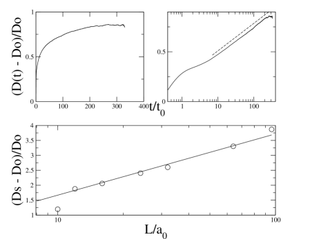
Figure 2: The top two plots show the temporal evolution of the self diffusion coefficient of a fluid particle in a large box of size $256a_{0}\times 256a_{0}$ with periodic boundary conditions. The right plot shows that rather than saturate, the diffusion coefficient grows as $D\sim\ln t$, as expected from theory. The bottom plot shows the hydrodynamic corrections to the diffusion coefficient $D$ compared to to the random collision approximation expression $D_{0}$ given by Eq (21) for different box sizes $L$. As expected, these corrections shows a logarithmic growth with $L/a_{o}$.

Before investigating the behavior of colloids in suspension, we study a simpler problem of an SRD fluid confined to two dimensions. Much of this section will follow on an earlier comprehensive study by Ripoll et al. Ripo05 in 3d, but here we focus on 2d.

We begin by deriving an expression for the velocity autocorrelation function of the SRD particles, following similar steps to those found in ref. Ripo05 for 3d. The $n^{th}$ collision step of the SRD method can be rewritten as

$${\bf{v}}_{i}(n\delta t_{c}) = {\bf{v}}_{i}((n-1)\delta t_{c})+(\mathcal{R}_{i}(\alpha)-\mathcal{I})$$ (8)

$$\times \left[{\bf{v}}_{i}((n-1)\delta t_{c})-{\bf{v}}_{c.m,i}((n-1)\delta t_{c})\right]$$

where $\mathcal{I}$ is the unit matrix, and $t=n\delta t_{c}$ the discretized time, with $n$ the number of collision steps, $\delta t_{c}$ the collision interval and ${\bf{v}}_{c.m,i}$ the cell center of mass velocity. The rotation matrix is defined in two dimensions as

$$\mathcal{R}_{i}(\alpha)=\left(\begin{array}[]{cc}\cos\alpha&\pm\sin\alpha\\ \mp\sin\alpha&\cos\alpha\end{array}\right)$$

such that the rotational average over any vector ${\bf{A}}$ becomes

$${\langle}(\mathcal{R}(\alpha)-\mathcal{I}){\bf{A}}{\rangle}=-(1-\cos\alpha){\bf{A}}=-\zeta_{\alpha}{\langle}{\bf{A}}{\rangle}.$$ (9)

If we now assume density fluctuations in each cell to be small, we can write ${\langle}{\bf{v}}_{c.m,i}(n\delta t_{c}){\rangle}\simeq\frac{1}{m\gamma}{\langle}{\sum_{j}^{i,n}\bf{v}}_{j}{\rangle}$. By multiplying each side by ${\langle}{\bf{v}}_{i}(0){\rangle}$ and further assuming the velocity of colliding particles to be uncorrelated, we arrive at

$${\langle}{\bf{v}}_{c.m,i}((n-1)\delta t_{c}){\bf{v}}_{i}(0){\rangle}\simeq\frac{1}{m\gamma}{\langle}{\bf{v}}_{i}((n-1)\delta t_{c}){\bf{v}}_{i}(0){\rangle}.$$ (10)

where $\gamma$ is the average number of solvent particles per cell. Substituting (10) and (9) into (8), and rearranging, we obtain an expression for the correlation of a fluid particle

$${\langle}{\bf{v}}_{i}(n\delta t_{c}){\bf{v}}_{i}(0){\rangle}=(1-\zeta_{\alpha}\zeta_{\rho}^{m}){\langle}{\bf{v}}_{i}((n-1)\delta t_{c}){\bf{v}}_{i}(0){\rangle}$$ (11)

where $\zeta_{\rho}^{m}=1-1/\gamma$. This expression shows that we can write the correlation at a certain time step in terms of the previous time step, such that the normalized velocity autocorrelation function (VACF) is,

$$\frac{{\langle}{\bf{v}}_{i}(n\delta t_{c}){\bf{v}}_{i}(0){\rangle}}{{\langle}{\bf{v}}^{2}_{i}(0){\rangle}}\simeq\zeta^{n}$$ (12)

where $\zeta=1-\zeta_{\alpha}\zeta_{\rho}^{m}$ is the decorrelation factor. The VACF, for reasons that will become apparent later, is the quantity of interest here and has the form

$${\langle}{\bf{v}}_{i}(n\delta t_{c}){\bf{v}}_{i}(0){\rangle}\simeq\frac{k_{B}T}{m}\zeta^{n}$$ (13)

A similar analysis can be performed for the case of a single heavy tracer particle of mass $m^{\prime}$ embedded in a solvent Ripo05 . The total mass in a collision box is then $(M+m\gamma)$ such that the center of mass correlation is written as

$${\langle}{\bf{v}}_{c.m,i}(n\delta t_{c}){\bf{v}}_{i}(0){\rangle}\simeq\frac{m^{\prime}}{m\gamma+M}{\langle}{\bf{v}}_{i}(n\delta t_{c}){\bf{v}}_{i}(0){\rangle}.$$ (14)

By substituting (14) into (11), the decorrelation factor for a heavy tracer particle is found to be

$$\zeta=1-\zeta_{\alpha}\frac{m\gamma}{m\gamma+m^{\prime}}=1-\zeta_{\alpha}\zeta_{\rho}^{M}.$$ (15)

The self diffusion constant $D$ of a particle $i$ is related to its mean square displacement via the Einstein relation Hansen86 :

$$D=\lim_{t\to\infty}\frac{1}{4t}{\langle}[{\bf{r}}_{i}(t)-{\bf{r}}_{i}(0)]^{2}{\rangle}.$$ (16)

The position of a particle can be written explicitly in terms of discrete time-steps

$${\bf{r}}_{i}(t)={\bf{r}}_{i}(0)+\delta t_{c}\sum^{n-1}_{k=0}{\bf{v}}_{i}(k\delta t_{c}),$$ (17)

so that

$${\langle}[{\bf{r}}_{i}(t)-{\bf{r}}_{i}(0)]^{2}{\rangle}=\delta t_{c}^{2}\sum^{n-1}_{j=0}\sum^{n-1}_{k=0}{\langle}{\bf{v}}_{i}(j\delta t_{c}){\bf{v}}_{i}(k\delta t_{c}){\rangle}.$$ (18)

We note that combining the equation above with Eq. (16) leads to the discrete form of the standard Green-Kubo expression for the diffusion coefficient as an integral over the velocity autocorrelation function. Manipulating the sums, we find Tuzel03

$$\sum^{n-1}_{j=0}\sum^{n-1}_{k=0} {\langle} {\bf{v}}_{i}(j\delta t_{c}){\bf{v}}_{i}(k\delta t_{c}){\rangle}$$

$$= \sum^{n-1}_{j=0}{\langle}{\bf{v}}_{i}^{2}(j\delta t_{c}){\rangle}+2\sum^{n-2}_{j=0}\sum^{n-1}_{k=j+1}{\langle}{\bf{v}}_{i}(j\delta t_{c}){\bf{v}}_{i}(k\delta t_{c}){\rangle}$$

$$= 2n\frac{k_{B}T}{m}+2\sum^{n-1}_{j=1}j{\langle}{\bf{v}}_{i}(0){\bf{v}}_{i}((n-j)\delta t_{c}){\rangle}.$$

Substituting the expression for the VACF derived earlier (13) into (III), we can write the diffusion coefficient in terms of its decorrelation factor $\zeta$,

$$D=\lim_{n\to\infty}\frac{k_{B}T}{m}\delta t_{c}\left[\frac{1}{2}+\frac{1}{n}\sum^{n-1}_{j=1}j\zeta^{n-j}\right]=\frac{k_{B}T\delta t_{c}}{2m}\left[\frac{1+\zeta}{1-\zeta}\right].$$ (20)

Substituting Eq.15 into Eq.20, results in the following dimensionless expressions for the self diffusion constant of a fluid and heavy tracer particle respectively

$$\frac{D_{0}^{m}}{D_{0}} = \lambda\left[\frac{1}{1-\cos\alpha}\left(\frac{m\gamma}{m\gamma-1}\right)-\frac{1}{2}\right]$$ (21)

$$\frac{D_{0}^{m^{\prime}}}{D_{0}} = \frac{\lambda m}{m^{\prime}}\left[\frac{1}{1-\cos\alpha}\left(\frac{\gamma+\frac{m^{\prime}}{m}}{\gamma}\right)-\frac{1}{2}\right].$$ (22)

$D_{0}$ denotes the unit of diffusion and is expressed as $a^{2}_{0}/t_{0}=a_{0}\sqrt{k_{B}T/m}$ and $\lambda$ is the dimensionless mean free path. It is a measure of the average distance the fluid particles travel in between collisions and has the form Padd06

$$\lambda=\frac{\delta t_{c}}{a_{0}}\sqrt{\frac{k_{B}T}{m}}=\frac{\delta t_{c}}{t_{0}}.$$ (23)

These expressions for $D$ make a key approximation, namely that collisions are always random, and that the particle velocities are uncorrelated. This neglects any hydrodynamic effects. These expressions are thus expected to become more accurate if the mean-free path $\lambda$ becomes larger so that the random collision approximation is expected to be a better description. Ripoll et al  Ripo05 showed that in 3d, for their simulation parameters, the expression (21) for self-diffusion of an SRD particle began to show significant deviations from measured values when the mean-free path was smaller than $0.6$. Similarly, they found that for smaller mean-free paths $\lambda=0.1$, these expressions could underestimate the diffusion coefficient of a tagged heavier particle of mass $M$ by as much as $75\%$ for $M\geq 10m$.

In Fig. 1 we analyze the self-diffusion coefficient of a tagged SRD particle as a function of mass and of mean free path for a square geometry with plates $L=32a_{0}$ SRD cell widths wide. Similarly to Ripoll et al. Ripo05 we find deviations due to hydrodynamics, but in 2d these are much more pronounced. For example, as the mass increases, the hydrodynamic corrections to Eq.21 saturate at a deviation of over $200\%$ for larger masses. Similarly, we observe larger deviations as a function of mean free path than found in 3d.

In contrast to the 3d results, for which finite size effects are not very strong, we expect that in 2d the effect of box size will be much more pronounced. To illustrate this, we carried out simulations in a much larger square box of width $L=256a_{0}$ box sizes, now with periodic boundary conditions. These are shown in the top two plots of Fig. 2. We observe that the temporal diffusion coefficient, defined as

$$D(t)=\int^{t}_{0}{\langle}v(t^{\prime})v(0){\rangle}dt^{\prime},$$ (24)

continues to grow with time in a manner consistent with the expected scaling $D\sim\ln[t]$, as illustrated in the second top plot in Fig. 2. We expect the diffusion coefficient to eventually saturate for this finite box size. But for an infinite box, we expect that $D(t)$ will continue to grow indefinitely, a manifestation of the Stokes Paradox. Similarly, for a fixed box of size $L^{2}$, we expect that $D\sim L/a_{0}$ Happ73 , as discussed in the introduction, and this scaling is indeed observed in the bottom panel in Fig. 2.

IV Velocity autocorrelation functions of colloidal particles

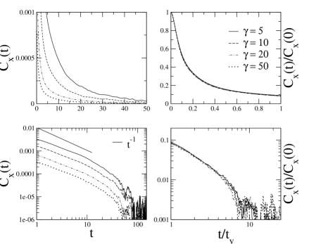
Figure 3: Scaling of the velocity autocorrelation function : when VACF is normalized and plotted in terms of the reduced time $t/t_{\nu}$, all the data collapse to the same curve. The VACF was originally measured for varying solvent densities $\gamma$. The system size is $L=32a_{0}$, which implies that $\chi_{s}=L/2\sigma_{cs}=8$.

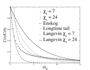
Figure 4: Normalized colloid VACFs simulated for increasing pipe width with $\chi_{s}=\frac{L}{2\sigma_{cs}}=7,24$, with $L=28,96a_{0}$. Simulations results were scaled with the Enskog time is $t_{E}=1.0888t_{0}$ calculated from (29). The dashed line represents the short time decay from (30), the dashed-dotted line represent the decay from the long time tail calculated from (27) whilst the dotted line and the solid line denote the Langevin decay with the friction $\xi$ for the two respective box sizes.

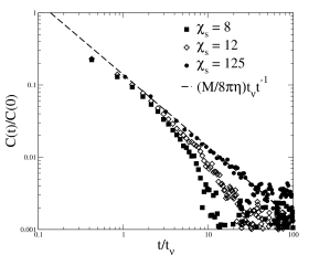
Figure 5: Log-log plot of the VACF for of a colloidal particle in boxes of size $L=32,48,500a_{0}$ ($\chi_{s}=8,12,125$). The dashed line is the fit from Eq.27 and serves as a guide to the eye.

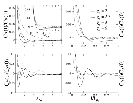
Figure 6: Normalized velocity autocorrelation function of a colloidal particle confined between two walls for increasing values of $\chi_{s}=L/2\sigma_{cs}$. Simulations here were performed for pipe widths $L=8,10,12,24a_{0}$. The different plots denote the components of the normalized VACF parallel $C_{x}(t)$ (top) and perpendicular $C_{y}(t)$ (bottom) to the walls. Note that all plots are scaled with the kinematic time $t_{\nu}=\sigma_{cs}^{2}/\nu$, and the time-scale for momentum to diffuse the distance between the walls $t_{w}=L^{2}/4\nu$. The minimum of the negative tails observed for $C_{x}(t)$ scale on top of each other when time is scaled with the sonic time $t/t_{cs}$ (insert in upper right panel). Similarly, the oscillating tails for $C_{y}(t)$ show the same period when scaled with $t/t_{W}$ (bottom right panel).

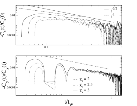
Figure 7: Log-log plot of the VACF of a confined colloidal particle for boxes of size $L=8,10,12a_{0}$ ( $\chi_{s}=2,2.5,3$ respectively). The dashed line and the straight line have slopes $t^{-1}$ and $t^{-3/2}$ respectively. Only the positive values of $-C(t)$ are plotted here.

Having worked out some properties of diffusing SRD particles, we now turn to the properties of colloidal particles embedded in a solvent.

If memory effects are ignored in a simple Langevin equation description of a spherical colloid of mass $M$, then the velocity autocorrelation function (VACF) of a colloidal particle can be calculated to be   Russ89

$${\langle}v(t)v(0){\rangle}=\frac{k_{B}T}{M}\exp(-t/t_{\xi}),$$ (25)

where the time $t_{\xi}=M/\xi$ indicates how quickly particles forget their initial velocity. Its integral is related to the diffusion coefficient through the Einstein relation:

$$D=\int^{\infty}_{0}{\langle}v(t)v(0){\rangle}dt=\frac{k_{B}T}{\xi}.$$ (26)

The Einstein relation is of course valid for any physical description of the VACF.

Langevin approaches have traditionally been used for colloidal systems when hydrodynamics could be ignored. However, it is well known that hydrodynamic effects can have an important qualitative effect on the VACF. In their pioneering work, Alder and Wainwright Alde70 used MD simulations to demonstrate that the VACF ($C(t)$) of a tagged particle exhibits an algebraic decay at long times of the form $t^{-d/2}$, instead of the exponential form predicted by the Langevin equation. They showed that this behavior was a consequence of momentum conservation, and therefore quite general. For colloidal particles in 3d, the diffusion coefficient is dominated by the contributions from this long time tail Padd06 , and we expect the same to be true in 2d. The correlation function for a colloid with slip boundary conditions can be calculated from kinetic theory  Alde70 :

$$\langle v(t)v(0)\rangle=\left(\frac{d-1}{d\rho}\right)\frac{k_{B}T}{(4\pi(D+\nu)t)^{d/2}},$$ (27)

where $d$ is the number of dimensions, and $\rho$ the solvent density. This calculation predicts a $t^{-1}$ power for the tail in 2 dimensions. That this should cause problems for the definition of $D$ is evident from Eq.26 because it implies that D diverges logarithmically with time. Note that similar behavior was seen for pure SRD particles in Fig. 2, where we found the scaling $D(t)\sim\ln[t]$. For the colloids, we expect that the tail in the VACF will form on the timescale $t_{\nu}=\sigma_{cs}^{2}/\nu$ it takes the kinematic viscosity $\nu$ to diffuse over the particle radius.

Fig.3 shows simulations run for a square box with a width $L=32a_{0}$. Eq.27 predicts that the tail should scale as $((\nu+D)\rho t)^{-1}$. We tested this further by varying the number density $\gamma$ and simultaneously changing the density of the colloids so that they remain buoyant. For SRD the kinematic viscosity $\nu$ depends only very weakly on $\gamma$ Pool04 ; Padd06 for large values of $\gamma$ and keeping in mind that from equipartition

$$C(0)={\langle}v(0)^{2}{\rangle}=\frac{k_{B}T}{M}$$ (28)

it is not hard to show that the long time tails should all scale onto the same curve if time is scaled with $t/t_{\nu}$. We show this explicitly in Fig. 3 for a fixed system size.

At times shorter than the kinematic time, there is a contribution to the overall diffusion that comes from the local random collisions between the colloid and the solvent particles. This is typically dominant on time scales less than the sonic time $t_{cs}=v_{s}/\sigma_{cc}$ over which collective modes can be generated Padd06 . We can calculate it using standard Enskog kinetic theory, and the ensuing Enskog friction coefficient $\xi_{E}$ has the following form Phd

$$\xi_{E}^{2d}=\frac{3\sqrt{2}}{4}\sigma_{cs}\gamma\pi^{3/2}\left(k_{B}T\frac{mM}{m+M}\right)^{1/2}$$ (29)

in two dimensions. Thus for very short times, the decay of the VACF is characterized by the Enskog time $t_{E}=M/\xi_{E}^{2d}$ and it follows that

$$\langle v(t)v(0)\rangle=\frac{k_{B}T}{M}\exp(-t/t_{E}).$$ (30)

because the collisions are essentially random.

As shown in Fig. 4, for short times, on the order of the Enskog time $t_{E}$, the autocorrelation function shows clear exponential decay, in good agreement with Eq.30. The simulations shown are for two box sizes, and for short times, the VACF are independent of system size, as expected from Enskog theory.

At longer times, Fig. 4 clearly shows the beginning of the long-time tail. The theoretical line we plot is from Eq. 27, and fits remarkably well to the data. However, we note that there are some small deviations with system size at these longer times, which will be explained below.

We also note that a direct comparison with the Langevin equation shows that for short times the Langevin equation overestimates the VACF, and that for longer times in underestimates the VACF for colloids. A more in depth discussion of this point can be found in appendix B of Ref I. In addition, in two dimensions, the Langevin equation (25) would predict an exponential form with different $t_{\xi}$ for different box sizes, because the diffusion coefficient changes with box size. By contrast, our results show that for short times the VACF is independent of box size. Clearly the Langevin equation does a poor job in capturing details of the colloidal VACF.

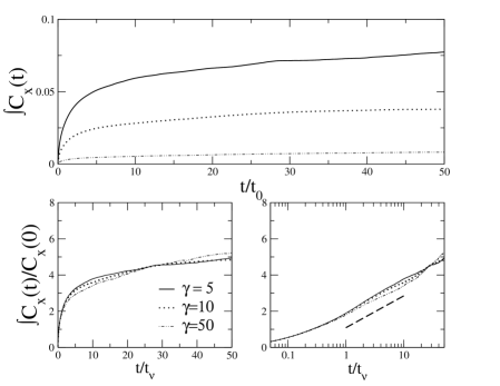
Figure 8: Time evolution of the time-dependent diffusion coefficient of a buoyant colloid in two dimensions for SRD particle densities $\gamma=5,10,50$. The bottom two graphs show the diffusion coefficient normalized by $C_{x}(0)=k_{B}T/M$, with time scaled by $t/t_{\nu}$. We expect the graphs to scale on to each other for longer times where the long-time tails dominate. (see also Fig. 3). The bottom right graph has a logarithmic scale and the dashed line has the slope $\frac{M}{8\pi\eta}$ and serves as a guide to the eye.

While the simulations above are for fixed boundaries, it is also interesting to see what happens to the VACF when the confinement is more pronounced. In confined geometries, the particle induced flow fields should feel the presence of the walls. Bocquet and Barrat Boc showed that a sink in the decay of the long time tails should occur after an observation time on the order of $t_{w}=\frac{L^{2}}{4\nu}=\chi_{s}^{2}t_{\nu}$. This time is characteristic of how long it takes for the kinematic viscosity to reach the wall, when $L/2$ is the average distance to the wall. We illustrate the effect of the wall on the VACF in Fig. 5 for three different box sizes. For the two narrower boxes, the VACF clearly begins to drop below the $t^{-1}$ power law but for the largest box, of size $L=500a_{0}$, we don’t observe any deviation within our error bars. The sink in the tail for the $\chi_{s}=8$ simulation run begins at an observation times less than $10t_{\nu}$, whereas the kinematic wall time in this instance is $t_{W}\approx 64t_{\nu}$. That may be because of other wall effects that kick in earlier for such a narrow box, or it may be that the cutoff in the algebraic decay is gradual and commences sooner than predicted by Bocquet and Barrat.

In an important study, Hagen et al  Pago01 used Lattice Boltzmann simulations to investigate the VACF of a colloidal particle between rigid walls and found qualitative deviations from the standard long-time tails. In particular, for a sphere in a narrow enough cylinder, they found negative tails for the VACF $C_{x}(t)$ parallel to the walls that exhibited an algebraic decay like $C_{x}(t)\sim t^{-3/2}$. Similarly, for a two dimensional disc between two plates they found $C_{x}(t)\sim t^{-3/2}$, and for a three dimensional sphere between two plates they found $C_{x}(t)\sim t^{-2}$. These exponents depend on the confinement, rather than on the overall dimension of the system. They explained the emergence of this negative tail with a simple mode-coupling theory that takes into account the fact that the sound wave generated by the colloid becomes diffusive. They further noticed that for slip walls, the normal behavior was recovered, suggesting the origin of the negative tail lies in the existence of velocity gradients near the wall.

We performed simulations of colloidal discs in a pipe of length $512a_{0}$ with periodic boundaries in the $x$ direction and with two stick boundary condition walls at a reduced distance $\chi_{s}=L/2\sigma_{cs}=2,2.5,3,6$, apart in the $y$ direction and show the results in Fig. 6. We find a negative tail for $C_{x}(t)$, the VACF parallel to the plates, We find that the amplitude of the negative tail grows with increasing confinement. Furthermore, when time is scaled with $t/t_{cs}$, the different correlation functions all show a minimum at about $t\approx 3t_{cs}$, suggesting that sound waves are indeed the dominant cause of the negative tail, as suggested in  Pago01 . For the larger confinement shown here, $\chi_{s}=6$, the VACF does show a rapid decay, but there does not seem to be a negative tail. This suggest that the diffusive sound wave mechanisms are still playing a part in the smallest ($\chi_{s}=8$) simulations of Fig. 5, and may explain why the VACF decays on a shorter time $t/t_{W}$ than predicted by Bocquet and Barrat Boc .

In the bottom two panels of Fig. 6 we observe oscillatory behavior for $C_{y}(t)$, the VACF perpendicular to the plates. This can be explained as follows: when a particle moves in the $y$ direction towards the wall, it sets up a momentum flow which can reflect off the wall and come back a time later to push the particle in the opposite direction. This effect should become more pronounced for stronger confinement, as we observe. To check this mechanism, we note that the walls introduce another length-scale, $t_{W}=\frac{L^{2}}{4\nu}$, which is the time it takes vorticity to diffuse to the walls. If this reflection mechanism is at play, we would expect the period of the oscillations to reflect this time-scale. In the bottom right panel of Fig. 6, we observe that when $C_{y}(t)$ is scaled with the time $t/t_{W}$ the oscillation minima indeed fall on top of each other, at least for sufficiently strong confinement.

As discussed by Hagen et al Pago01 , the $C_{x}(t)$ should exhibit a negative tail that scales like $t^{\frac{-3}{2}}$ for sufficiently strong confinement. In the upper plot of Fig. 7 we indeed observe that the exponent is greater than $t^{-1}$, and consistent with $t^{-\frac{3}{2}}$, as expected, although our data is not clean enough to confirm the exact exponent. Similarly, the final decay of the component $C_{y}(t)$ appears closer to $t^{-1}$ than to $t^{-\frac{3}{2}}$.

Clearly confinement has an important effect on the long-time behavior of the VACF, and there may be further subtle effects that we have not yet been uncovered. It would be interesting, for example, to see how the angular correlation functions, studied in ref. Padd05 with SRD for 3d stick boundary colloids in the bulk phase, would behave under confinement. However, for the calculation of long-time tails, methods like Lattice Boltzmann techniques used by Hagen et al. Pago01 , where noise does not play a big role, may be simpler and faster to use.

V Diffusion coefficient of colloidal particles under confinement

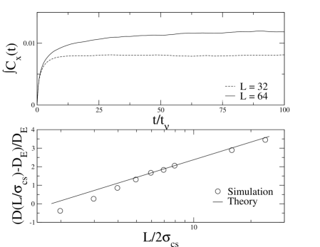
Figure 9: Top : The effect of confinement on diffusion. The two curves represent the temporal evolution of the self diffusion coefficient for colloids in varying confinement. The dashed line denotes colloids diffusing between plates a distance $L=32a_{0}$ apart ($\chi_{s}=8$) whilst in the case of the solid line the plate separation is $64a_{0}$ ($\chi_{s}=16$). For the smaller pipe, the kinematic wall time is $t_{W}\approx 64t_{\nu}$. The diffusion coefficient begins to plateau much earlier than that because the effect of the wall on the VACF kicks in earlier than that. Note that only the x-component of the diffusion is plotted here. Bottom : Simulations were performed for 2d pipes of respective widths $L=8,12,16,20,24,28,32,64,96a_{0}$. The straight line is the fit from (V.2) and the circles are the simulation points.

The Einstein relation (26) directly relates the VACF and the diffusion coefficient. We found that for short times, the VACF was well described by an Enskog form (30) that was largely independent of the boundaries, and that at longer times it exhibited a long time tail that was much more sensitive to the boundaries. For strong confinement, the tail could even be negative or oscillatory, but for weak confinement, it appears to scale as $C(t)\sim t^{-1}$.

For an unbounded 2d system, the diffusion coefficient does not converge, instead its behavior with time can be approximated as:

$$D^{2d}(t) = \int^{t}_{0}{\langle}v(t)v(0){\rangle}dt$$ (31)

$$\approx \frac{k_{B}T}{M}\left(\int^{t_{\nu}}_{0}\exp(-t/t_{E})dt\right)+\int^{t}_{t_{\nu}}\frac{k_{B}T}{8\pi\rho\nu t}$$

$$\approx \frac{k_{B}T}{\xi^{2d}_{E}}+\frac{k_{B}T}{8\pi\eta}\left[\ln t\right]^{t}_{t_{\nu}}$$

where we have assumed that the Enskog and hydrodynamic contributions to the VACF can be separated (this is not quite true) and moreover that the hydrodynamic tail does not kick until a time scale on the order of the kinematic time $t_{\nu}$. We also assume that $D\ll\nu$.

V.1 Simulations in the ’bulk’

In Fig. 8, we present the temporal evolution of the self diffusion coefficient of a colloid for a large box. We approximated colloids in the bulk by using a box of size $L^{2}=256a_{0}\times 256a_{0}$ with periodic boundary conditions. The plot shows results for solvent densities $\gamma=5,10,50$. On the time-scales of the simulation, we observe behavior consistent with $D\sim\ln[t]$, as expected from the $t^{-1}$ tail of the VACF. In practice this would mean that $D$ would grow indefinitely with time, and be unbounded, which is a manifestation of the Stokes Paradox.

V.2 Simulations in confinement

Whereas the diffusion coefficient of a two dimensional disc in the bulk appears to grow in an unbounded fashion with time, the diffusion coefficient for a confined fluid is expected to saturate at a finite value Happ73 ; Boc . We showed in Figs 3 - 7 that the VACF is affected by the presence of walls, and no longer shows the $t^{-1}$ behavior at very long times that would lead to a logarithmic divergence. As a result of the wall interaction, the diffusion will no longer diverge, but will plateau at a value determined by the distance to the wall.

We tested this simple argument by simulating colloids under two different levels of confinement. The top panel of Fig. 9 shows the integral of the velocity autocorrelation function plotted for colloids diffusing between parallel plates a distance $L=32a_{0}$ and $L=64a_{0}$ apart respectively. For the smaller system, the temporal diffusion coefficient reaches a plateau at shorter times than is found for the larger system.

To make these arguments more quantitative, we make the following approximation to the diffusion coefficient:

$$D^{2d}(L/\sigma_{cs}) \sim \int^{t_{W}}_{0}{\langle}v(t)v(0){\rangle}dt$$

$$\approx \frac{k_{B}T}{\xi_{E}^{2d}}+\frac{k_{B}T}{8\pi\eta}\left[\ln t\right]^{t_{W}}_{t_{\nu}}$$

$$= D_{E}+\frac{k_{B}T}{8\pi\eta}\ln\frac{t_{W}}{t_{\nu}}$$

$$= D_{E}+\frac{k_{B}T}{4\pi\eta}\ln\frac{L}{\sigma_{cs}}$$

which indicates that the diffusion of a particle in confinement should scale with the log of the ratio of its radius to the pipe width.

We performed simulations to check the validity of this simple scaling argument. The results are shown in Fig. 9, and can be accurately fitted to Eq.(V.2).

While Eq.V.2 works very well for the larger boxes, it overestimates the diffusion coefficient for the smaller boxes. This is because the more complex wall effects shown in Fig 6 come into play so that the VACF no longer shows simple $t^{-1}$ behavior assumed in Eq.V.2. We also note that in the smallest systems studied, the Enskog contribution is more than half of the overall diffusion (although this is not the reason for the deviation from the simple $\ln[L/\sigma_{cs}]$ scaling).

It was shown by Bungay and Brenner Bung73 using standard methods of low Re number hydrodynamics, that the diffusion coefficient of a sphere in a 3d pipe of radius $R_{p}$ drops rapidly with $R_{p}/R_{c}$. Here we see from direct simulations of the VACF and the diffusion coefficient that the same behavior can be seen in 2d. It also drops as a function of decreasing pipe width. It would be interesting to see if similar hydrodynamic arguments to those used by Bungay and Brenner Bung73 could be used to explain the more rapid decrease of the diffusion coefficient observed in 2d for stronger confinement.

VI Conclusion

We have applied the SRD simulation method to the study of the dynamics of two dimensional disks in confined geometries. We calculated the VACF for colloids and observed the predicted $t^{-1}$ behavior as well as the more complex oscillating behavior and negative tails in strong confinement. We also observed the logarithmic dependence of the diffusion coefficient on system size, as originally predicted by Saffman Saff76 for the lateral diffusion of a cylinder in a film.

Although the Saffman result describes the motion of a disk of thickness $h$, and our simulation deals with disks, we can still map our results onto a real physical system by equating the diffusion coefficient measured in our simulations to that measured in experiment.

Through this study we have shown that SRD can be fruitfully used to simulate colloids in two dimensions. This suggests that it could easily be adapted for the study of other problems, such as protein and lipid molecules in biological membranes Cone72 ; Cone73 ; Cone74 ; Edidin74 ; Pete82 , liquid domains in giant unilamellar vesicles (GUVs) Cicu07 , or colloids in a liquid film Cheu96 ; DiLe08 , or various examples from microfluidics Squi05 .

- (1) G. G. Stokes, Trans. Cambridge Philos. Soc. 9, 8 (1851). Reprinted in Mathematical and Physical Papers, 2nd ed., Vol. 3 (Johnson Reprint Corp., New York, 1966).
- (2) Cited in H. Lamb, Hydrodynamics, (CUP, Cambridge, 1932), p 614.
- (3) P.G. Saffman and M. Delbruck, Proc. Nat. Acad. Sci. 72, 311 (1975); P.G. Saffmann, J. Fluid Mech. 73, 593 (1976).
- (4) R. A. Cone, Nature New Biol. 236, 39, (1972).
- (5) M. Poo, R. A. Cone Exp. Eye Res. 17 503, (1973).
- (6) M. Poo, R. A. Cone Nature 247 438, (1974).
- (7) M. Edidin, Annu. Rev. Biophys. Bioeng. 3, 179 (1974).
- (8) R. Peters and R.J. Cherry, Proc. Natl. Acad. Sci. 79 4317 (1982).
- (9) P. Cicuta, S. L. Keller, S. L. Veatch; Journ. Phys. Chem. Lett B. 111 3328 (2007).
- (10) C. Cheung, Y.H. Hwant, X-l. Wu, and H.J. Choi Phys. Rev. Lett. 76, 2531 (1996).
- (11) R. Di Leonardo, S. Keen, F. Ianni, J. Leach, M.J. Padgett, and G. Ruocco, Phys. Rev. E 78 031406 (2008).
- (12) J. Happel and H. Brenner, Low Reynolds Number Hydrodynamics (Springer, 1973). E. Guazzelli, Phys. Fluids 7, 12 (1995). 2574 (1997).
- (13) A. Malevanets and R. Kapral, J. Chem. Phys. 110, 8605 (1999).
- (14) T. Ihle and D. M. Kroll, Phys. Rev. E 67, 066705 (2003); T. Ihle and D.M. Kroll, Phys. Rev. E 67, 066706 (2003).
- (15) J. T. Padding and A. A. Louis, Phys. Rev. E. 74, 031402 (2006).
- (16) A. Malevanets and R. Kapral, J. Chem. Phys. 112, 7260 (2000).
- (17) J. T. Padding and A. A. Louis, Phys. Rev. Lett. 93, 220601 (2004); J.T. Padding and A.A. Louis, Phys. Rev. E. 77, 011402 (2008).
- (18) M. Hecht, J. Harting, T. Ihle, and H. J. Herrmann, Phys. Rev. E 72, 011408 (2005).
- (19) M. Ripoll, K. Mussawisade, R.G. Winkler, and G. Gompper, Phys. Rev. E 72, 016701 (2005).
- (20) T.S. Squires and S.R. Quake, Rev. Mod. Phys. 77, 977 (2005).
- (21) E. S. Boek, J. Chin and P. V. Coveney, Int. Journ. Mod. Phys. B 17, 99 (2003).
- (22) M. Venturoli, E. S. Boek, Elsevier Physica A 362 23, (2006).
- (23) G. A. Bird, Phys. Fluids 13, 2676 (1970).
- (24) G.A. Bird, Molecular Gas Dynamics and the Direct Simulation of Gas Flows (Claredon Press, Oxford, 1994).
- (25) A. Succi, The Lattice Boltzmann Equation for Fluid Dynamics and Beyond, Oxford University Press, Oxford (2001).
- (26) A.J.C. Ladd, Phys. Rev. Lett. 70, 1339 (1993)
- (27) A.J.C. Ladd and R. Verberg, J. Stat. Phys. 104, 1191 (2001).
- (28) M.E. Cates et al., J. Phys.: Condens. Matter 16, S3903 (2004); R. Adhikari1, K. Stratford, M. E. Cates, and A. J. Wagner, Europhys. Lett. 71, 473 (2005); K. Stratford et al., Science 309, 2198 (2005).
- (29) V. Lobaskin and B. Dünweg, New J. of Phys. 6, 54 (2004); V. Lobaskin, B. Dünweg, and C. Holm, J. Phys.: Condens. Matt. 16, S4063 (2004).
- (30) F. Capuani, I. Pagonabarraga, and D. Frenkel, J. Chem. Phys. 121, 973 (2004).
- (31) A. Chatterji and J. Horbach, J. Chem. Phys. 122, 184903 (2005).
- (32) C.P. Lowe, Europhys. Lett. 47, 145 (1999).
- (33) N. Kikuchi, C. M. Pooley, J. F. Ryder, and J. M. Yeomans, J. Chem. Phys. 119, 6388 (2003).
- (34) C.M. Pooley and J.M. Yeomans, J. Phys. Chem. B 109, 6505 (2005).
- (35) M. P. Allen and D. J. Tildesley, Computer simulation of liquids (Clarendon Press, Oxford, 1987)
- (36) J. T. Padding, A. Wysocki, H. Löwen, and A. A. Louis, J. Phys.:Condens. Matter 17, S3393 (2005).
- (37) J. P. Hansen, I. R. McDonald Theory of Simple Liquids Academic Press Inc. (1986)
- (38) E. Tüzel, M. Strauss, T. Ihle, D.M. Kroll, Phys. Rev.E, 68, 036701 (2003).
- (39) W. B. Russell, D. A. Saville, and W. R. Showalter, Colloidal Dispersions (Cambridge University Press, Cambridge, England, 1989).
- (40) B.J. Alder and T.E. Wainwright, Phys. Rev. A 1, 18 (1970).
- (41) M.H.J. Hagen, I. Pagonabarraga, C.P. Lowe, D. Frenkel: Phys. Rev. Lett 78, 3785 (1997).
- (42) J. Sané, Phd Thesis (to be published) (2008). y
- (43) L.Bocquet, J-L. Barrat: J. Phys. Condens. Matter 8, 9297 (1996)
- (44) P.M. Bungay and H. Brenner, Int. J. Multiph. Flow 1, 25 (1973).