Nonlinear dynamics and chaos Transport properties Wave propagation in random media

Transmission thresholds in time-periodically driven nonlinear disordered systems

Abstract

We study energy propagation in locally time-periodically driven disordered nonlinear chains. For frequencies inside the band of linear Anderson modes, three different regimes are observed with increasing driver amplitude: 1) Below threshold, localized quasiperiodic oscillations and no spreading; 2) Three different regimes in time close to threshold, with almost regular oscillations initially, weak chaos and slow spreading for intermediate times, and finally strong diffusion; 3) Immediate spreading for strong driving. The thresholds are due to simple bifurcations, obtained analytically for a single oscillator, and numerically as turning-points of the nonlinear response manifold for a full chain. Generically, the threshold is nonzero also for infinite chains.

Energy transport is rather well understood in linear discrete Hamiltonan systems, where general solutions are linear combinations of eigenmodes, and the transport properties are completely determined by the nature of the spectrum of eigenfrequencies and the corresponding eigenmodes. For spatially periodic systems the linear spectrum is absolutely continuous and the eigenmodes are planewaves, implying that any initially localized wavepacket will generally disperse throughout the system, with amplitude vanishing to zero at infinite time. Conversely, when the linear system is strongly disordered we have Anderson localization, characterized by a purely discrete linear spectrum with square summable (localized) eigenmodes. Then, initially localized wavepackets do not spread to zero and there is no energy diffusion.

The aim of this paper is to understand how some aspects of the transport properties of systems with linear Anderson localization are affected when nonlinearity is added. Obviously, for a nonlinear system, general solutions are not just linear combinations of eigenmodes. Still however, special (time-periodic) solutions generally exist, which continue single linear eigenmodes from the small-amplitude limit, and thus in some sense correspond to nonlinear eigenmodes. Due to the nonlinearities, the frequency of such a continued solution varies with amplitude, and each time it crosses a resonant linear eigenfrequency a new peak appears at the location of the corresponding linear mode. Since there are infinitely many resonant frequencies in any finite frequency interval, the continued solution develops infinitely many new peaks, and thus the strict continuation of a localized Anderson mode becomes a spatially extended mode for any non-zero amplitude [1]. Experimentally, such nonlinear delocalization was reported in [2] for a two-dimensional fiber array. At larger amplitude, the spatial density of the peaks increases so that even in-between peaks the amplitude is never small, thus allowing the transportation of a substantial energy current by phase torsion [3]. However, despite the existence of these extended solutions it has been shown [4, 5, 6], that spatially localized time periodic solutions also persist with nonlinearities, but when the frequency is inside the linear band they are not in strict continuation of the linear modes. Instead, the frequency of a localized solution becomes a discontinuous function of its amplitude, with a gap located near each linear eigenfrequency. Although there are infinitely many gaps since the eigenfrequencies form a dense set in the spectrum, the gap widths become exponentially small as functions of the spatial distance of the resonance location, and as a consequence the “allowed” frequencies belong to a (fat) Cantor set with nonzero measure [4]. Indications of experimental excitation of a sequence of such “intraband discrete breathers” were given in [2]. Finally, when the nonlinearity is strong enough to drive the frequency outside the linear band, “extraband discrete breathers” (discrete solitons) are formed, and localization is generally enhanced as has been seen experimentally for several types of photonic lattices [2, 7, 8]

Thus, this indicates that nonlinearities on one hand maintain the existence of localized solutions which could trap energy forever, but on the other hand also generate new extended solutions which could transport energy. To investigate the possible energy diffusion, numerical experiments have studied the time evolution of an initially localized wave packet [9, 10, 11, 12, 13, 14]. This may be analyzed by expanding the solutions in the basis of Anderson modes, which then become coupled by nonlinear terms. It was early conjectured [9] that this coupling, if strong enough, would allow the energy to diffuse from one Anderson mode to another, leading to a (subdiffuse) spread throughout the system. Several numerical studies apparently confirmed that the second moment of the energy distribution of a single wave packet may diverge as a function of time [10, 11]. However, this does not necessarily imply that its amplitude vanishes at infinite time. By observing the time evolution of the participation number, which measures the localization length of the core of the wavepacket, it was shown [12] that for large enough initial amplitude the participation number remains finite, although the second moment may diverge if some part of the energy spreads to infinity. The observations in [12] also suggested that the wavepacket may have a limit profile (possibly with infinite second moment) which is an almost periodic solution (with a discrete Fourier transform) and zero Lyapunov coefficients analogous to KAM tori in finite systems. This conjecture is supported by rigorous results proving the existence of such solutions in random DNLS systems [15, 16].

This paper is devoted to another test for the energy transport property: the transmission through a system with a time periodic driving force locally applied. While the above arguments referred to finite energy wavepackets in systems at zero temperature, the external driving force now acts as an energy source. We have investigated several nonlinear models with linear Anderson localization, but focus on two prototype examples: the Discrete Nonlinear Schrödinger (DNLS) and Fermi-Pasta-Ulam (FPU) models, in both cases with driving at a single edge site of a semi-infinite chain. Numerically, we choose the chain length $N$ to be sufficiently large to have no observable change when increasing $N$. Since we aim at describing a qualitative scenario generically valid for any typical disordered chain, we do not average over different realizations.

A DNLS chain with random on-site potential and non-parametric periodic (harmonic) driving at a boundary site is described by the dynamical equations

$$\mathrm{i}\dot{\psi}_{n}-V_{n}\psi_{n}+C(\psi_{n+1}+\psi_{n-1})+|\psi_{n}|^{2}\psi_{n}=A_{n}\mathrm{e}^{\mathrm{i}\omega t},$$ (1)

where $C$ is the coupling constant, and the amplitude $A_{n}=A\delta_{n0}$ of the driving force at frequency $\omega$ is non-zero only at site $n=0$. We take $V_{n}$ to be random variables with uniform distribution in the interval $[-V,+V]$. This gives a linear spectrum (for undriven chain) between $[-2C-V,+2C+V]$. The explicit time-dependence of the force in eq. (1) is removed by transforming to a frame rotating with frequency $\omega$, $\psi_{n}(t)=\phi_{n}(t)\mathrm{e}^{\mathrm{i}\omega t}$, yielding

$$\mathrm{i}\dot{\phi}_{n}-(\omega+V_{n})\phi_{n}+C(\phi_{n+1}+\phi_{n-1})+|\phi_{n}|^{2}\phi_{n}=A_{n}.$$ (2)

For a given initial condition $\phi_{n}(0)$, there are three independent parameters: $A/C$ (driving strength), $V/C$ (disorder strength), $\omega/C$ (driving frequency). (We may always put $C=1$ by rescaling time and wavefunction.) Equation (2) can be derived from the Hamiltonian

$$\mathcal{H}=\sum_{n=0}^{+\infty}\left\{(\omega+V_{n})|\phi_{n}|^{2}-C(\phi_{n+1}\phi_{n}^{*}+\phi_{n+1}^{*}\phi_{n})\right.$$

$$\left.-\frac{1}{2}|\phi_{n}|^{4}+A_{n}\phi_{n}^{\ast}+A_{n}^{*}\phi_{n}\right\},$$ (3)

since $\mathrm{i}\dot{\phi}_{n}=\frac{\partial{\mathcal{H}}}{\partial\phi_{n}^{\ast}}$, $\mathrm{i}\dot{\phi}^{\ast}_{n}=-\frac{\partial{\mathcal{H}}}{\partial\phi_{n}}$. Thus, even in presence of driving ${\mathcal{H}}$ is a conserved quantity, characterizing the initial condition. If we choose ${\phi_{n}}(0)\equiv 0$ and apply the driving instantaneously at $t=0$, then $\mathcal{H}=0$. However, if we slowly increase the force from zero to its final value $A$ during a transient time, then $\mathcal{H}$ is not constant during the transient, and generally $\mathcal{H}\neq 0$ after the transient. We measure the ”amount of excitation” in the system at a given time from the total norm (or power in optics)

$${\mathcal{N}}(t)=\sum_{n}|\phi_{n}|^{2},$$ (4)

which is a conserved quantity only in absence of driving.

If all parameters $|A/C|$, $|V_{0}/C|$, $|\omega/C|$ are large, we can neglect the coupling to the rest of the lattice and only consider the single anharmonic oscillator at $n=0$:

$$\mathrm{i}\dot{\phi}_{0}-(\omega+V_{0})\phi_{0}+|\phi_{0}|^{2}\phi_{0}=A.$$ (5)

The nature of stationary solutions (constant $|\phi_{0}|$) to eq. (5) is wellknown (see, e.g., ref. [17]). Due to conservation of $\mathcal{H}$, it is integrable. Expressing $\phi_{0}=r_{0}\mathrm{e}^{\mathrm{i}\theta_{0}}$ ($r_{0}\geq 0$ and $\theta_{0}$ real) yields $\dot{r}_{0}=-A\sin{\theta_{0}}$; $\dot{\theta}_{0}+\omega+V_{0}-r_{0}^{2}=-\left(A/r_{0}\right)\cos\theta_{0}$. Thus, a stationary solution ($\dot{r}_{0}=0$) in presence of driving ($A\neq 0$) can only exist if $\theta_{0}=0$ or $\pi$, corresponding to oscillations inphased resp. antiphased to the driving force. They are obtained by solving the cubic equation $r_{0}^{3}-(\omega+V_{0})r_{0}\mp A=0$, where upper (lower) sign corresponds to $\theta=0$ ($\pi$). When $A=0$, the solutions are $r_{0}=0$ (”linear solution”, $\mathcal{H}=0$) and $r_{0}=\sqrt{\omega+V_{0}}$ if $\omega+V_{0}>0$ (”nonlinear solution”, $\mathcal{H}=(\omega+V_{0})^{2}/2$). For $A>0$, the cubic equation for $\theta=0$ always has one (stable) solution for $r_{0}\geq 0$, which continues the ”nonlinear solution” towards larger $r_{0}$ when $\omega+V_{0}>0$ and the ”linear solution” when $\omega+V_{0}<0$. In addition, for small $A>0$ and $\omega+V_{0}>0$ the cubic equation for $\theta=\pi$ has two solutions with $r_{0}>0$, one stable continuing the ”linear solution” towards larger $r_{0}$ and one unstable continuing the ”nonlinear solution” towards smaller $r_{0}$. However, at a critical driving strength $A=A^{(c)}=2(\omega+V_{0})^{3/2}/\left(3\sqrt{3}\right)$ these solutions bifurcate, so that for $A>A^{(c)}$ only the ”nonlinear solution” with $\theta=0$ remains.

The significance of this bifurcation is, that if $A$ is increased slowly (adiabatically) from zero for a zero initial condition when $\omega+V_{0}>0$, the solution will follow the stable solution with $\theta=\pi$ until it disappears at $A=A^{(c)}$. Above this threshold the solution cannot jump dynamically to the other stable stationary solution with $\theta=0$ since it has larger ${\mathcal{H}}$, but instead $r_{0}$ becomes periodic with a new oscillation frequency (corresponding to a quasiperiodic solution in the non-rotating frame). By contrast, for $\omega+V_{0}<0$ there is always only one solution which continues the ”linear solution” for all $A$.

For the full chain, an analogous threshold can be described by the nonlinear response manifold (NLRM) technique, used in [5, 6] to calculate time-periodic breathers for a non-driven disordered lattice, and in [18] to analyze transmission thresholds in driven nonrandom Klein-Gordon chains [19]. For the 1D DNLS model, it can be simply implemented numerically. Looking for real (i.e., carrying no current) stationary solutions with $\dot{\phi_{n}}=0$, eq. (2) can be written as a 2D map with $x_{n}=\phi_{n}$, $y_{n}=\phi_{n+1}$, which we may iterate backwards from $n=N$ to $n=1$,

$$\left(x_{n-1},y_{n-1}\right)=\left(\frac{(\omega+V_{n}-x_{n}^{2})}{C}x_{n}-y_{n},x_{n}\right).$$

Using as map initial (boundary) condition $(x_{N},y_{N})=(0,\epsilon)$ for a number of different $\epsilon$ (typically $\sim 1000$ with max $\epsilon$ $\sim 10^{-12}$ for $N\simeq 50-100$ sites) gives a number of points belonging to a manifold at the end of iteration at $(\phi_{0},\phi_{1})$. Combining this with the equation at the edge site $n=0$, $A=-(\omega+V_{0}-x_{0}^{2})x_{0}+Cy_{0}$, and plotting, e.g., $x_{0}=\phi_{0}$ as a function of $A$ gives a projection of the NLRM, from which we may obtain all real stationary solutions at given driving strength $A$ as intersections of the NLRM with the vertical line at $A$. (The above set of map initial conditions yields only half the NLRM, the other half is obtained by adding $\phi_{0}(-A)=-\phi_{0}(A)$ but in order to not overload the figures it is not shown below) As discussed in [18], each turning point (TP) of the NLRM can be associated with a threshold-like behaviour. Increasing the system size may yield more loops in the NLRM, but the structure of the first loops, and in particular the first TP, are generally found to remain unchanged for $N\gtrsim 100$.

We now illustrate numerically, how these NLRM TPs are related to transmission thresholds in the dynamics. Attempting to adiabatically follow the continuation of the linear stationary (i.e., with same frequency as driving force) solution as long as it exists, we increase the driving strength slowly from zero to its final value. as $A(t)=A(1-\mathrm{e}^{-t/\tau})$, with typically $\tau\sim 100-1000$. We choose a rather strong disorder, $V=2.5$, in order to have well localized linear modes (we put $C=1$). To be concrete, we show results obtained for one particular realization of the disorder, for which the on-site potential of the driving site is $V_{0}\approx 2.48977$.

Figure 1: (a) (Half) NLRM for a random DNLS chain with $V=2.5$ and $\omega=0$. The apparent line through the origin is in fact a very thin loop, continuing the linear solution from the origin towards negative $A$ until it reaches the first TP at $(-1.9411,0.697025)$ (inset in (a)). It then returns to the right, crosses $A=0$ at a small positive $\phi_{0}$, reaches a second TP at (2.17, -0.97), and then escapes towards large negative values (not shown). (b) Time evolution of norm (main figure) and participation number (inset) for, from bottom to top, $A=1.5$, $A=1.9$ (just below first TP), $A=2.0$ (between first and second TP), and $A=2.2$ (above second TP). Transient time $\tau=100$. (c), (d): Shape of the solution for $A=1.9$, showing (c) the first transition from almost regular to slowly spreading, and (d) the second transition to strongly diffusive, behaviour.

In fig. 1 we show (half) the NLRM and time-evolution of total norm (4) and participation number $P={\mathcal{N}}^{2}/\sum|\phi_{n}|^{4}$ for different $A$ for a driving frequency in the middle of the linear band, $\omega=0$.

When the driving strength is far below the first TP of the NLRM ($A=1.5$ in fig. 1(b)), the response is essentially linear-like and, if the force is increased sufficiently slowly, the solution is essentially a stationary solution at the driving frequency, localized close to the driving site and belonging to the stable (lower) branch of the first (left) thin bifurcation loop in fig. 1(a)). The small (quasiperiodic) oscillations are due to non-adiabaticity, and will decrease if $\tau$ is increased. Thus, this represents the sub-threshold-type of non-transmitting dynamics. We have confirmed that this regular behaviour remains also for considerably longer integration times, e.g., $10^{6}$.

For $A$ just below the first TP (fig. 1(c), (d)), we observe a critical behaviour, where the small oscillations due to non-adiabaticity generally are weakly chaotic and cause the orbit to slowly diffuse in phase-space. At $t\sim 5000$ it jumps to a different phase-space region, with bounded but larger oscillations (fig. 1(c)). We associate this with the existence of a neighboring stable stationary solution on the second loop of the NLRM (these solutions are close due to the thinness of the first loop). However, finally ($t\sim 13000$, fig. 1(d)), the solution escapes into a continuously spreading, strongly chaotic state with rapid increase of ${\mathcal{N}}$ and $P$. A similar scenario is observed also for $A$ between the first and second TPs ($A=2.0$ in fig. 1(b)), although in this case the weakly chaotic oscillations always develop as soon as $A$ passes the first TP, even for larger $\tau$.

Finally, for $A$ above the second TP ($A=2.2$ in fig. 1(b)), the spreading starts essentially immediately, and relevant measures like norm and participation number generally grow as $t^{\alpha}$, where $\alpha$ is close to 0.5 indicating a diffusive-like behaviour (for some different cases we obtained exponents between approximately 0.44 and 0.60).

Figure 2: Adiabatic threshold $A_{\mathrm{th}}(\omega)$, determined from the first TP of the NLRM, for the same DNLS chain as in Fig 1. The resolution in $\omega$ is $10^{-4}$ and chain length $N=100$.

The main qualitative features discussed above are generic, although in particular the quantitative behaviour in the critical regime depends on the detailed structure of the NLRM, which for other parameter values may be considerably more complicated than in fig. 1(a). But generally, for each random chain (fixed disorder realization and $V$) we can identify an adiabatic transmission threshold $A_{\mathrm{th}}(\omega)$ from the first TP of the NLRM, remembering that the real observed threshold is somewhat smaller due to nonadiabatic effects (finite $\tau$). The dependence $A_{\mathrm{th}}(\omega)$ exhibits sharp variations, as shown in fig. 2 for the chain used in fig. 1. For an infinite chain, $A_{\mathrm{th}}(\omega)$ is conjectured to be an upper semicontinuous function (larger than or equal to its limit at any point), which should become zero at any frequency resonant with a linear mode (i.e., on a dense set of points), but nonzero for most frequencies and in average. In fig. 2 we can clearly observe the stronger resonances corresponding to modes located close to the driving site, while weaker resonances from distant modes should cause similar effects more difficult to observe numerically. We also confirmed that the transmission threshold decreases towards zero when approaching the lower band edge, as indicated by fig. 2. However, for frequencies smaller than the smallest resonance frequency (lower band edge for an infinite system, and $\omega\approx-2.7$ for the finite system in fig. 2), there is no TP at all of the NLRM, and the numerical simulations show complete absence of transmission even for very large driving forces.

To illustrate that the above scenario is indeed generic, and not due to special DNLS properties like conservation of ${\mathcal{H}}$, we now discuss a random FPU chain with $N$ sites and a cubic nonlinear force. The equations of motion are

$$\ddot{u}_{n}=K_{n}(u_{n+1}-u_{n})-K_{n-1}(u_{n}-u_{n-1})$$

$$+(u_{n+1}-u_{n})^{3}-(u_{n-1}-u_{n})^{3},$$ (6)

where $u_{n}$ is the displacement of site $n$ and $K_{n}$ are random coupling constants, independent and uniformly distributed in $[K_{\mathrm{min}},K_{\mathrm{max}}]$. In the following we fix $K_{\mathrm{min}}=1$ and $K_{\mathrm{max}}=4$ (we put $K_{0}=1$). To simulate an impinging wave we impose on one end the boundary condition $u_{0}(t)=A\cos\omega t$, while free boundary conditions, $u_{N+1}=u_{N}$, are enforced on the other side of the chain.

An important difference between the FPU and DNLS models is that, with free boundary conditions on both sides, the FPU linear eigenmodes are well localized only for large enough frequencies, since the localization length $\xi$ diverges as $\xi\sim\omega^{-2}$ in the limit $\omega\to 0$ [20]. More precisely, in a chain of $N$ sites, all eigenvectors for which [20]

$$\omega\;<\;\omega_{\mathrm{L}}\;\equiv\;\sqrt{\frac{8\langle K^{-1}\rangle}{N(\langle K^{-2}\rangle-\langle K^{-1}\rangle^{2})}}$$ (7)

are in practice extended (phonon) modes. Therefore, we consider driving frequencies in the upper part of the linear spectrum, $\omega_{\mathrm{L}}<\omega<\omega_{\mathrm{max}}$ where $\omega_{\mathrm{max}}$ is the band-edge.

In a series of numerical experiments we initialized the chain at rest ($u_{n}\equiv\dot{u}_{n}\equiv 0$) and increased smoothly the driving amplitude from 0 to $A$ with a constant rate, $u_{0}=A\cos(\omega t)\left[1-\mathrm{e}^{-t/\tau}\right]$, with typically $\tau=10$. To simulate a semi-infinite lattice and observe a stationary state in the transmission regime, we steadily removed the energy injected from the driver by adding a damping term $-\gamma\dot{u}_{n}$ to eq. (6) for a number $N_{D}$ of rightmost sites ($\sim 10\%$ of the total). As indicator, we used the local energy flux

$$j_{n}=\frac{1}{2}(\dot{u}_{n}+\dot{u}_{n+1})\left[K_{n}(u_{n+1}-u_{n})+(u_{n+1}-u_{n})^{3}\right].$$ (8)

After a transient of $\sim 1000$ driver periods, the site- and time-averaged energy flux $\overline{j}=\left(\sum_{n=1}^{N-N_{D}}\overline{j_{n}}\right)/\left(N-N_{D}\right)$ was computed (the bar denotes time average). Figure 3 shows results for several values of $\omega$ ($\omega\gg\omega_{\mathrm{L}}\sim 0.44$), for a fixed disorder realization. As in the DNLS case, a well-defined transmission threshold $A_{\mathrm{th}}$ exists for every frequency.

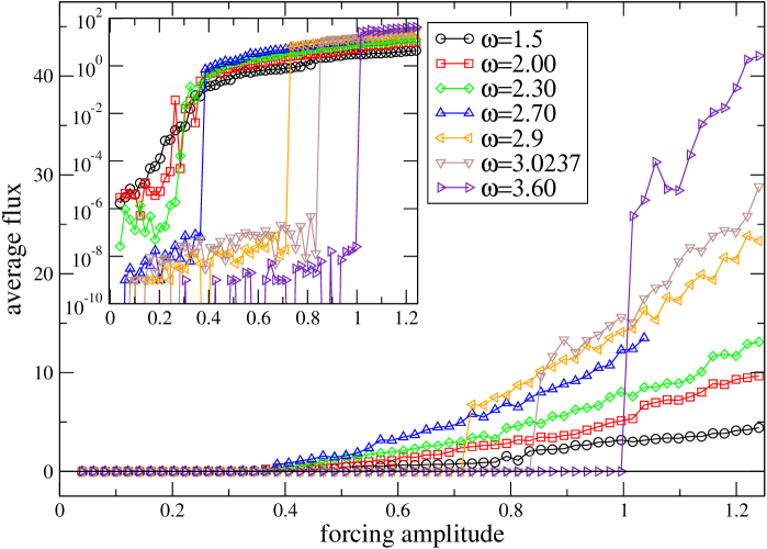
Figure 3: Average fluxes $\overline{j}$ versus amplitude driving $A$ for different frequencies $\omega$. $N=512$, $N_{D}=50$, $\gamma=0.1$. The averages are performed on about $2\cdot 10^{4}$ periods. Inset: same data in lin-log scale. Notice that the jump can be six orders of magnitude.

Its exact value depends on the specific disorder realization (becoming small if there is a resonant mode close to the edge), but the qualitative behaviour is the same. Moreover, $A_{\mathrm{th}}$ is insensitive to variations of the size $N$ (we checked sizes between $N=512$ and $N=4096$) and dissipation at damped sites $N_{D}$. Similarly to the DNLS case (cf. fig. 2 and the analytical result $A^{(c)}$ for a single oscillator), there is an average tendency (disregarding the individual resonances) for $A_{\mathrm{th}}$ to increase with increasing frequency; note however that in the transmitting regime, the flux for a given driver amplitude increases with $\omega$.

Also for FPU the threshold is related to a TP of the NLRM, which may be easily computed in a rotating-wave approximation (a more computationally expensive exact calculation could be done analogously to refs. [5, 6, 18]). Looking for solutions of the form $u_{n}(t)=U_{n}\cos\omega t$ and approximating $\cos^{3}\omega t\approx(3/4)\cos\omega t$ in eq. (6), we get

$$-\omega^{2}U_{n}=K_{n}(U_{n+1}-U_{n})-K_{n-1}(U_{n}-U_{n-1})$$

$$+\frac{3}{4}(U_{n+1}-U_{n})^{3}-\frac{3}{4}(U_{n-1}-U_{n})^{3}.$$ (9)

This equation can be solved with respect to $U_{n}-U_{n-1}$ yielding a two dimensional backward map $(U_{n-1},V_{n-1})=(U_{n}-F(V_{n},U_{n}),U_{n})$, where the function $F$ is obtained by solving a cubic equation.

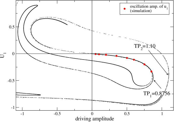
Figure 4: Projection of the approximate FPU NLRM, obtained by iterating a few hundred points in an interval of size $\epsilon\sim 10^{-8}$ around the origin, for $\omega=3.0237$ and the same disorder realization as in fig. 3. Large points show the maximal oscillation amplitudes of the first particle, measured from simulation.

In fig. 4 we show the last iterate $(U_{0},V_{0})$ (note that $U_{0}=A$) of a set of trajectories started along the unstable manifold of the origin. The curve is locally linear around $A=0$ (linear response) and then bends and turns wildly similar as discussed above. This computed manifold agrees very well with the data obtained from simulation when the driving is switched on very slowly (here $\tau=400$). As can be seen, the first TP ($TP_{1}$ in fig. 4) is at $A=0.8756$ which is in excellent agreement with the observed transmission threshold 0.878.

Below threshold energy does not propagate and, as in the DNLS case, only a few sites close to the driven boundary oscillate. As shown in fig. 5 their motion is quasiperiodic, with spectra displaying peaks at frequencies of the form $m_{1}\Omega_{1}+\ldots+m_{p}\Omega_{p}$. Each site oscillates with a different set of frequencies $\Omega_{i}$. To characterize the localization properties of the quasiperiodic state we computed the time-averaged energy density $\overline{e}_{n}$,

$$e_{n}\;=\;\frac{\dot{u}^{2}_{n}}{2}+\frac{1}{2}\left[V_{n+1}(u_{n+1}-u_{n})+V_{n}(u_{n}-u_{n-1})\right],$$ (10)

with $V_{n}(x)=K_{n}x^{2}/2+x^{4}/4$. As seen in fig. 6, it displays a slow decay along the chain compatible with a power-law, $\overline{e}_{n}\propto n^{-3.3}$. A tail with similar exponent was found also when averaging over some different disorder realizations in the nontransmitting regime. Presumably, this is due to the presence of long-wavelength almost extended modes in the linear spectrum [20]; in DNLS an exponential decay is generally seen for the sub-threshold quasiperiodic state.

Figure 5: Fourier power spectra of the velocities $\dot{u}_{n}$ at sites $n=1,5,10$ for $\omega=3.0237$ and $A=0.850$ (just below threshold). The insets show the Poincaré sections $(u_{n}(kT),\dot{u}_{n}(kT))$ ($k$ integer) where $T=2\pi/\omega$ is the driving period.

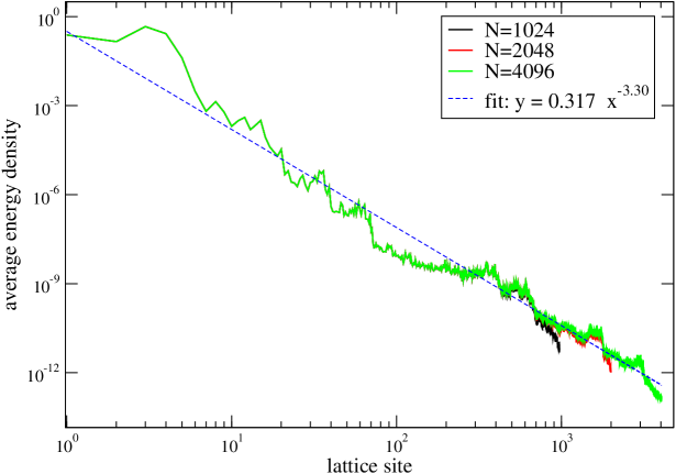
Figure 6: The time-averaged energy profile $\overline{e}_{n}$ below threshold, for $A=0.83322$, $\omega=3.0237$ and different lattice sizes. Other parameters like in figs. 3-5.

The interpretation of the threshold as a transition from quasiperiodicity to chaos can be seen in the Fourier spectra of $\dot{u}_{n}$ as an immediate broadening of the lines for $A>A_{\mathrm{th}}$. Asymptotically, for the transmitting state $\overline{e}_{n}$ is found to reach a given profile as in the ordered case [21], reminiscent of stationary heat transport with two thermal baths [22].

In summary, we have shown the existence of well-defined transmission thresholds for generic classes of locally time-periodically driven nonlinear disordered Hamiltonian chains. An adiabatic threshold for the driver amplitude can be defined from the associated NLRM, and is nonzero except at a discrete set of resonant frequencies. Applying the force nonadiabatically generates quasiperiodic solutions in the nontransmitting regime, and lowers the transmission threshold. Beyond the threshold, energy is transmitted diffusively through a chaotic state. These thresholds could be directly observable, e.g., in optical waveguide arrays [23, 8] and for Bose-Einstein condensates in disordered potentials [24]. Although we here focused on two particular models, we have found qualitatively similar results also for random Klein-Gordon lattices [5, 6, 18] and the parametrically driven DNLS model [25]. A recent work [26] also reported a transmission threshold in a model similar to eq. (1), but with dissipation at both edges. However, while ref. [26] argues that their threshold in average should decrease to zero in the limit of an infinite chain, a major conclusion from our work is that the threshold generically remains nonzero also in the limit $N\rightarrow\infty$ for any typical disorder realization. This follows also from the fact that the NLRM generally has a finite slope at the origin (except for the zero-measure set of resonant frequencies), which was proven in ref. [6] under basic smoothness assumptions. The existence of a smooth NLRM in the thermodynamic limit could possibly also be rigorously proven, at least for the DNLS case, as a consequence of the Ruelle-Oseledec theorem.

This work was initiated within the Advanced Study Group 2007 Localizing energy through nonlinearity, discreteness and disorder at the MPIPKS, Dresden. S.L. acknowledges useful discussions with S. Ruffo. M.J. acknowledges support from the Swedish Research Council. G.K. and S.A. thank the Greek GSRT and Egide for support through the Platon program.

References

- [1] \NameKopidakis G. Aubry S. \REVIEWPhysica D1301999155.
- [2] \NamePertsch T. et al. \REVIEWPhys. Rev. Lett.932004053901.
- [3] \NameAubry S. \REVIEWPhysica103D1997201.
- [4] \NameAlbanese C. Fröhlich J. \REVIEWCommun. Math. Phys.1161988475; 138 (1991) 193; \NameAlbanese C., Fröhlich J. Spencer T. \REVIEWibid.1191988677.
- [5] \NameKopidakis G. Aubry S. \REVIEWPhys. Rev. Lett.8420003236.
- [6] \NameKopidakis G. Aubry S. \REVIEWPhysica D1392000247.
- [7] \NameSchwartz T. et al. \REVIEWNature446200752.
- [8] \NameLahini Y. et al. \REVIEWPhys. Rev. Lett.1002008013906.
- [9] \NameShepelyansky D.L. \REVIEWPhys. Rev. Lett.7019931787.
- [10] \NameMolina M.I. \REVIEWPhys. Rev. B58199812547.
- [11] \NamePikovsky A.S. Shepelyansky D.L. \REVIEWPhys. Rev. Lett.1002008094101.
- [12] \NameKopidakis G. et al. \REVIEWPhys. Rev. Lett.1002008084103.
- [13] \NameGarcía-Mata I. Shepelyansky D.L. \REVIEWPhys. Rev. E792009026205.
- [14] \NameFlach S., Krimer D.O. Skokos Ch. \REVIEWPhys. Rev. Lett.1022009024101.
- [15] \NameFröhlich J., Spencer T. Wayne C.E \REVIEWJ. Stat. Phys.421986247.
- [16] \NameBourgain J. Wang W.-M. \REVIEWJ. Eur. Math. Soc. 1020081.
- [17] \NameRigo M. et al. \REVIEWPhys. Rev. A5519971665.
- [18] \NameManiadis P., Kopidakis G. Aubry S \REVIEWPhysica D2162006121.
- [19] \NameGeniet F. Leon J. \REVIEWPhys. Rev. Lett.892002134102.
- [20] \NameMatsuda H. Ishii K \REVIEWSuppl. Prog. Theor. Phys.45197056.
- [21] \NameKhomeriki R., Lepri S. Ruffo S. \REVIEWPhys. Rev. E702004066626.
- [22] \NameLepri S., Livi R. Politi A. \REVIEWPhys. Rep.37720031.
- [23] \NameKhomeriki R. \REVIEWPhys. Rev. Lett.922004063905.
- [24] \NamePaul T. et al. \REVIEWPhys. Rev. A722005063621.
- [25] \NameHennig D. \REVIEWPhys. Rev. E5919991637.
- [26] \NameTietsche S. Pikovsky A. \REVIEWEPL84200810006.