Transition from mode-locked periodic orbit to chaos in a 2D piecewise smooth non-invertible map

Abstract

In this work we report a new route to chaos from a resonance torus in a piecewise smooth non-invertible map of the plane into itself. The closed invariant curve defining the resonance torus is formed by the union of unstable manifolds of saddle cycle and the points of stable cycle and saddle cycle. We have found that a cusp torus cannot develop before the onset of chaos, though the loop torus appears. The destruction of the two-dimensional torus occurs through homoclinic bifurcation in the presence of an infinite number of loops on the invariant curve. We show that owing to the non-invertible nature of the map, the structure of the basin of attraction changes from simply connected to a nonconnected one. We also describe how the mechanism of transition to chaos differs from the scenario of appearance of chaos in invertible maps as well as in smooth non-invertible maps.

I Introduction

Piecewise smooth (PWS) maps have received much research attention in the recent times because of their applicability in a large number of practical systems S. Banerjee and G. C. Verghese (2001); Z. T. Zhusubaliyev and E. Mosekilde (2003); M. di Bernardo et al. (2007). This includes switching circuits S. Banerjee and C. Grebogi (1999), impact oscillators B.Brogliato (1999); J. Ing et al. (2008), a variety of micro and macro economic systems J. Laugesen and E. Mosekilde (2006), cardiac dynamics C. M. Berger et al. (2007) and many other systems. For such maps a particular kind of bifurcation may occur, which is different from what can occur in smooth maps. As a control parameter changes, the fixed point may move in the phase space and may collide with the borderline between two smooth regions, resulting in an abrupt jump of the Floquet multipliers from the inside of the unit circle to the outside of it in the complex plane, leading to a special class of nonlinear phenomena known as border collision bifurcation (BCB) H. E. Nusse and J. A. Yorke (1992); H. E. Nusse et al. (1994); S. Banerjee and C. Grebogi (1999); M. di Bernardo et al. (1999); P. Kowalczyk (2005).

The BCB consists of many atypical phenomena such as direct transition from a period-$1$ attractor to a chaotic attractor S. Banerjee and C. Grebogi (1999), multiple attractor bifurcation M. Dutta et al. (1999) and dangerous BCB Hassouneh et al. (2004). Recently in a series of papers Z. T. Zhusubaliyev et al. (2006); Z. T. Zhusubaliyev et al. (2008a, b) a new type of BCB has been reported, where a stable fixed point changes into an unstable focus along with an attracting closed invariant curve. This closed invariant curve forms a torus associated with quasiperiodic or phase-locked periodic dynamics Z. T. Zhusubaliyev et al. (2006). Moreover, the torus breakdown route to chaos in PWS invertible map has been characterized in Z. T. Zhusubaliyev et al. (2008a) which is distinct from that of Afraimovich-Shilnikov V. S. Afraimovich and L. P. Shilnikov (1991). These mechanisms of the creation and destruction of tori were studied in the context of two-dimensional smooth invertible maps D. G. Aronson et al. (1982) and PWS invertible maps Z. T. Zhusubaliyev et al. (2008a).

In another line of work V. Maistrenko et al. (2003); E. N. Lorenz (1989); C. E. Frouzakis et al. (2003), the occurrence of chaos via torus destruction has been studied numerically and experimentally for non-invertible smooth maps. Several routes to chaos were reported. The basic theory was proposed by Maistrenko et al. V. Maistrenko et al. (2003) and Lorenz E. N. Lorenz (1989). In transition from a smooth invariant curve (IC) to a chaotic attractor, the process begins with the IC developing segments with increasingly high curvature. At a certain parameter value cusps develop on the IC, which subsequently change into loops. With further change of the parameter, the IC can be destroyed in accordance with scenarios analogous to those of the invertible case. After that the chaotic attractor comes into existence. Cusps appear on IC when the degree of a map is greater than one and the IC intersects the critical curve so that the tangent of the IC at the point of intersection coincides with the eigenvector corresponding to zero eigenvalue or the critical curve contains cusp point (a point on a curve at which tangents of each branch of the curve coincide). Critical curve is the two dimensional extension of the local extrema (critical point) of a one dimensional differentiable map. It is the locus of all those points at which Jacobian determinant vanishes. For a non-differentiable piecewise linear map like the tent map, the point of non-differentiability plays the role of critical point. But for a two dimensional piecewise smooth map, according to Mira et al. C. Mira et al. (1996) the critical curve $LC$ is the image of the borderline $LC_{-1}$ of the map and is characterized by the set of all points which have at least two coincident rank-$1$ preimages. This curve may contain more than one segment. It separates the phase plane into open regions where all points of a region have the same number of rank-$1$ preimages.

The two dimensional PWS normal form maps S. Banerjee and C. Grebogi (1999); Z. T. Zhusubaliyev et al. (2008a) investigated so far are invertible. In the present paper we are interested in the dynamical behavior of non-invertible PWS maps. Considering a general piecewise linear 2D map expressed in the normal form, we derive the parameter regions where the map is non-invertible. We illustrate how chaos appears in PWS non-invertible maps and demonstrate the difference from the corresponding mechanisms of transition for smooth invertible D. G. Aronson et al. (1982) and non-invertible maps V. Maistrenko et al. (2003); E. N. Lorenz (1989). We investigate the bifurcation that takes place as one moves from the inside of a resonance tongue to the outside in the parameter space. Inside a resonance tongue, a closed invariant curve is formed by the saddle-node connections of a pair of cycles (a saddle and a node). This curve forms the mode-locked torus. We show that the cusp torus does not develop but the loop torus V. Maistrenko et al. (2003) is created before the destruction of mode-locked torus as the parameter is varied continuously. The mode-locked torus is destroyed through a homoclinic bifurcation. We observe that the interaction between stable manifold and the critical curve leads to a qualitative change in the basin of attraction, from a simply connected to a nonconnected one. We also show that the unstable manifolds can have structurally stable self-intersections while the stable manifolds can intersect itself when the map becomes structurally unstable. There is a coexistence of stable node and a chaotic attractor. We show that the size of basin of attraction of the stable cycle (node) diminishes to zero and after this the stable node undergoes a border collision fold bifurcation. We also illustrate the important role played by non-invertibility of the map in the mechanism of transition to chaos.

II Considered system

For a piecewise smooth map whose leading-order Taylor term close to the border is linear, the dynamics in the neighborhood of the border can be expressed by a normal form map S. Banerjee and C. Grebogi (1999); H. E. Nusse and J. A. Yorke (1992) defined by

$$F:\left(\begin{array}[]{c}x\\ y\end{array}\right)\rightarrow\left\{\begin{array}[]{cc}F_{1}(x,y)&\mbox{if}\;\;x\leq 0\\ F_{2}(x,y)&\mbox{if}\;\;x\geq 0\end{array}\right.$$ (1)

where

$$F_{1}(x,y)=\left(\begin{array}[]{c}\tau_{L}x+y+\mu\\ -\delta_{L}x\end{array}\right),$$

$$F_{2}(x,y)=\left(\begin{array}[]{c}\tau_{R}x+y+\mu\\ -\delta_{R}x\end{array}\right),\;\;(x,y)\in\mathbb{R}^{2}.$$

The phase plane $\mathbb{R}^{2}$ is divided into two compartments $L:=\{(x,y)\in\mathbb{R}^{2}:x\leq 0\}$ and $R:=\{(x,y)\in\mathbb{R}^{2}:x>0\}$. $\tau_{L}$ and $\delta_{L}$ are the trace and determinant respectively of the Jacobian matrix $J_{L}$ in the left half-plane $L$, and $\tau_{R}$ and $\delta_{R}$ are the trace and determinant respectively of the Jacobian matrix $J_{R}$ in the right half-plane $R$, and $\mu$ is a parameter. Thus

$$J_{L}=\left(\begin{array}[]{cc}\tau_{L}&1\\ -\delta_{L}&0\end{array}\right)\;\;\mbox{and}\;\;J_{R}=\left(\begin{array}[]{cc}\tau_{R}&1\\ -\delta_{R}&0\end{array}\right).$$

Most of the theories of BCB discussed so far are on dissipative dynamical systems (i.e., $|\delta_{L}|<1$, $|\delta_{R}|<1$). In contrast, we consider a situation where the map is contracting in the left side and expanding in the right side of the border, which happens when $|\delta_{L}|<1$, $|\delta_{R}|>1$. We choose $\tau_{L},\;\tau_{R}$ satisfying the conditions

$$-(1+\delta_{L})<\tau_{L}<(1+\delta_{L}),\;\;\;-2\sqrt{\delta_{R}}<\tau_{R}<2\sqrt{\delta_{R}}.$$ (2)

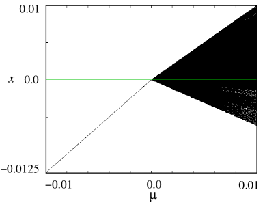
Figure 1: Bifurcation diagram obtained by varying the parameter $\mu$ from $-0.01$ to $0.01$. This diagram illustrates the birth of a quasiperiodic orbit after the border collision, directly from a stable fixed point for $\delta_{L}=-0.3$, $\delta_{R}=1.4$, $\tau_{L}=-0.1$ and $\tau_{R}=-0.685$.

The above conditions ensure that the fixed point for $\mu<0$ is attracting and for $\mu>0$ it is a spiral repellor. According to the notations in M. di Bernardo et al. (1999), we can write the stable fixed point by $A$ and unstable fixed point by $a$ in $L$, and similarly by $B$ and $b$ respectively in $R$. The fixed point in $L$ is

$$A\;or\;a=(\frac{\mu}{1-\tau_{L}+\delta_{L}},\frac{-\mu\delta_{L}}{1-\tau_{L}+\delta_{L}})$$

and the fixed point in $R$ is

$$B\;or\;b=(\frac{\mu}{1-\tau_{R}+\delta_{R}},\frac{-\mu\delta_{R}}{1-\tau_{R}+\delta_{R}}).$$

$A$ or $a$ exists if ${\mu}/{(1-\tau_{L}+\delta_{L})}\leq 0$, otherwise a virtual fixed point is located in $R$ and is denoted by $\bar{A}$ or $\bar{a}$. Similarly $B$ or $b$ exists if ${\mu}/{(1-\tau_{R}+\delta_{R})}\geq 0$, otherwise a virtual fixed point is located in the $L$ side and is denoted by $\bar{B}$ or $\bar{b}$. The stability of the fixed points is given by the eigenvalues

$$\lambda_{1},\lambda_{2}=\frac{1}{2}(\tau\pm\sqrt{\tau^{2}-4\delta}).$$

As the parameter $\mu$ hits the border at $\mu=0$, a stable fixed point $A$ on the $L$ side becomes an unstable focus $b$ on the $R$ side. When the outward spiraling orbit in the $R$ side touches the boundary of the $L$ side then it is attracted by the virtual fixed point $\bar{A}$ located in $R$. So the outward motion is arrested. This gives rise to the existence of an invariant closed curve on which stationary state must lie. Fig. 1 displays the bifurcation diagram varying the parameter $\mu$ from a negative to a positive value. This diagram depicts an abrupt transition from periodic to quasiperiodic behavior at a border-collision bifurcation.

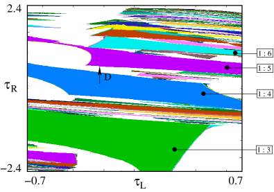
Figure 2: Regions of the periodic tongues in the ($\tau_{L},\tau_{R}$) parameter plane for $\delta_{L}=-0.3$, $\delta_{R}=1.4$ and $\mu=0.05$. Distinct colors of the tongues denote different oscillatory motions.

We plot the different resonance tongues in ($\tau_{L},\tau_{R}$) parameter plane for a positive value of $\mu$ (see Fig. 2). The main resonance tongues are denoted with the corresponding rotation numbers. Inspection of this figure reveals the presence of different periodic tongues which are densely spread in the parameter space. Yang and Hao Yang Wei-ming and Hao Bai-lin (1987) described the lens-like resonance tongues for a one-dimensional piecewise linear system, which were later generalized for two and three dimensional piecewise smooth systems in Z. T. Zhusubaliyev and E. Mosekilde (2003); Z. T. Zhusubaliyev et al. (2002); D. J. W. Simpson and J. D. Meiss (2008). The tongues are bounded by the curves where the stable and unstable cycles merge and disappear through BCB. A tongue may contain more than one lens.

III Properties of the considered non-invertible map

Proposition $1$. The two dimensional piecewise smooth normal form map (1) is non-invertible, if either $\delta_{L}$ and $\delta_{R}$ are of opposite sign, or any one of $\delta_{L}$ and $\delta_{R}$ is zero.

Proof. Since our map is continuous in $\mathbb{R}^{2}$, so we have to derive the conditions from one to one property. Let us suppose

$$X_{1}=\left(\begin{array}[]{c}x_{1}\\ y_{1}\end{array}\right),\;X_{2}=\left(\begin{array}[]{c}x_{2}\\ y_{2}\end{array}\right)\;\mbox{and}\;X_{1},\;X_{2}\in\mathbb{R}^{2}.$$

There are three possibilities.

Case I: $X_{1}$, $X_{2}$ $\in{L}$.

Now $F_{1}(X_{1})=F_{1}(X_{2})$
$\Rightarrow\tau_{L}x_{1}+y_{1}+\mu=\tau_{L}x_{2}+y_{2}+\mu\;$ $\mbox{and}\;-\delta_{L}x_{1}=-\delta_{L}x_{2}$.
$\Rightarrow x_{1}=x_{2}\;$(if$\;\delta_{L}\neq 0$) $\mbox{and}\;y_{1}=y_{2}$ .
So $F_{1}$ is one-one if $\delta_{L}\neq 0$.

Case II: $X_{1}$, $X_{2}$ $\in{R}$.

By a similar argument as in Case I, we conclude that $F_{2}$ is one-one if $\delta_{R}\neq 0$.

Case III: $X_{1}$ $\in{L}$, $X_{2}$ $\in{R}$.
$F_{1}(X_{1})=F_{2}(X_{2})$
$\Rightarrow\tau_{L}x_{1}+y_{1}+\mu=\tau_{R}x_{2}+y_{2}+\mu\;$ $\mbox{and}\;-\delta_{L}x_{1}=-\delta_{R}x_{2}$.
$\Rightarrow x_{1}=(\delta_{R}/\delta_{L})x_{2}\;$(if $\;\delta_{L}\neq 0$).

(a) If $\delta_{L}$ and $\delta_{R}$ are of the same sign and are non-zero.

Since $x_{1}\leq 0$ and $x_{2}>0$, the relation $x_{1}=(\delta_{R}/\delta_{L})x_{2}\;$ cannot hold. Therefore there can exist no points $X_{1}\in{L}$, $X_{2}\in{R}$ such that $F_{1}(X_{1})=F_{2}(X_{2})$. Hence the map is invertible.

(b) If $\delta_{L}$ and $\delta_{R}$ are of opposite sign.

The condition $x_{1}=(\delta_{R}/\delta_{L})x_{2}$ may hold.

Then $F_{1}(X_{1})=F_{2}(X_{2})$ $\Rightarrow{X_{1}\neq X_{2}}$ because $x_{1}\leq 0$ and $x_{2}>0$. Hence the map is non-invertible. Combining the above three cases the map is non-invertible if one of the following relations is satisfied

$(i)$ $\delta_{L}$ and $\delta_{R}$ are of opposite sign;

$(ii)$ any one of $\delta_{L}$ and $\delta_{R}$ is zero. $\;\;\Box$

To consider a typical non-invertible case, we assume $\delta_{L}=-0.3$ and $\delta_{R}=1.4$. Each point in $\mathbb{R}^{2}$ is mapped under (1) to a point in $\mathbb{R}^{2}$ with $y$-coordinate less than or equal to zero. There are two inverses for $(x,y)$ in $\mathbb{R}^{2}$ with $y\leq 0$. These are defined as

$$F^{-1}_{1}(x,y)=\left(\begin{array}[]{c}(-1/{\delta_{L}})y\\ x+(\tau_{L}/\delta_{L})y-\mu\end{array}\right)\;\mbox{and}$$

$$F^{-1}_{2}(x,y)=\left(\begin{array}[]{c}(-1/{\delta_{R}})y\\ x+(\tau_{R}/\delta_{R})y-\mu\end{array}\right),$$

where $(x,y)\in\mathbb{R}^{2}$ and $y\leq 0$.

Hence a point in $\mathbb{R}^{2}$ has two distinct rank-$1$ preimages if $y<0$, no preimage if $y>0$ and two coincident preimages if $y=0$. Let $Z_{0}$ be the region with no preimage (the upper half plane) and $Z_{2}$ be the region with two different preimages (the lower half plane). Thus for our choice of parameters, the map is of $Z_{0}-Z_{2}$ type C. Mira et al. (1996). The locus of the points having two merging rank-$1$ preimages is the $x$-axis, called $LC$. Here $LC$ is the critical curve. The preimages of each point in $LC$ lie on the $y$-axis, named as $LC_{-1}$. So the non-invertible map folds the phase plane along $LC$. The fixed points, periodic orbits and attractor must lie inside $Z_{2}$, because every fixed point and every point of a periodic orbit have an inverse (namely itself). A point on an attractor also has a preimage lying on that attractor.

IV Structure of the Stable and Unstable manifolds

Let $f:\mathbb{R}^{2}\rightarrow\mathbb{R}^{2}$ be a non-invertible smooth map and $x$ be a hyperbolic period-$q$ point of $f$. We define the stable manifold of $x$ as $W^{s}(x)=\{y\in\mathbb{R}^{2}:f^{nq}(y)\rightarrow x\;\mbox{as}\ n\rightarrow\infty\}$ and the unstable manifold of $x$ as $W^{u}(x)=\{y\in\mathbb{R}^{2}:f^{-nq}(y)\rightarrow x\;\mbox{as}\ n\rightarrow\infty\}$. These are defined in the neighborhood of $x$, and hence so are actually the local stable and unstable manifolds of $x$ C. Robinson (1999). The global unstable manifold is formed by the union of forward images of the local unstable manifold. It is connected, since the local unstable manifold is connected and the image of a connected set under continuous map is connected. The global unstable manifold is forward invariant but may not be backward invariant (some of its points have multiple preimages) and so self-intersections are allowed. The global stable manifold is formed by the union of all preimages of any rank of the local stable manifold. Since the map $f$ is non-invertible, the global stable manifold is backward invariant, but it may be strictly mapped into itself (some of its points may have no preimage). So it may be disconnected. For non-invertible maps the use of the term “manifold” is an abuse of the terminology; the local stable and unstable manifolds are guaranteed to be true manifolds, but the global manifolds are not C. E. Frouzakis et al. (1997); C. Robinson (1999). Still for our map we denote the global stable and unstable manifolds as the stable and unstable manifolds respectively.

Since our map $F$ is of $Z_{0}-Z_{2}$ type and the local unstable manifold originates at the saddle point $x$, it must lie in the $Z_{2}$ region. The unstable manifold is grown by iterating the local unstable manifold forward in time, every point computed will have a preimage, namely the previous point iterated to arrive at that point and hence the unstable manifold will never leave the $Z_{2}$ region (see Fig. 3(a)). The stable manifold is the union of all preimages of local stable manifold, connected or disjoint, so it can lie inside the $Z_{0}$ region also (see Fig. 3(a)).

V Transition to chaos in the presence of homoclinic structure

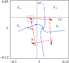
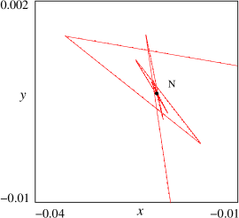
(a)               (b)

Figure 3: (a) Phase portrait of the attractor at $\tau_{R}=0.25$ with $\tau_{L}=-0.3$, $\delta_{L}=-0.3$, $\delta_{R}=1.4$ and $\mu=0.05$. (b) Enlargement of a portion of the IC marked by the square in (a). Points of stable cycles are marked with solid black circles, points of saddle cycles with open circles and the spiral repellor is marked with solid green circle.

Let us now analyze the bifurcational transition from mode-locking to chaos. To illustrate this scenario, we vary the bifurcation parameter $\tau_{R}$ from the inside of the $1:4$ tongue to the outside of it along the direction $D$ (see Fig. 2). The reason for this choice is that, the transition to chaos maintains the loop like structure as described by Maistrenko et al. V. Maistrenko et al. (2003) which we want to explain. Fig. 4(a) displays the bifurcation diagram and Fig. 4(b) depicts the Lyapunov exponents corresponding to the bifurcation diagram. The largest Lyapunov exponent becomes positive at $\tau_{R}\approx 0.5$, which implies the existence of a chaotic attractor. The second Lyapunov exponent remains negative over the considered parameter range. Initially the map (1) has a period-$4$ stable cycle and a period-$4$ saddle cycle. As the parameter $\tau_{R}$ increases, between $\tau^{h}_{R}\approx 0.5$ and $\tau^{c}_{R}\approx 0.57414$ the stable period-$4$ cycle coexists with a chaotic attractor. So we observe hard hysteretic transitions from periodic mode to chaotic mode and vice versa, at the points $\tau^{h}_{R}$ and $\tau^{c}_{R}$ respectively. At $\tau^{c}_{R}$ one of the points of the period-$4$ stable cycle and a point of the period-$4$ saddle cycle hit the border together. Then the period-$4$ stable and saddle cycles disappear through border collision fold bifurcation.

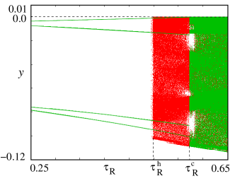
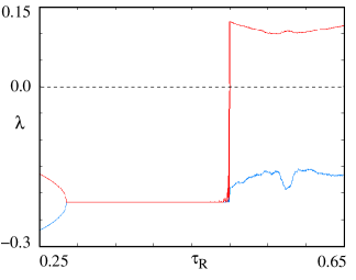
(a)           (b)

Figure 4: (a) Bifurcation diagram illustrating the birth of a chaotic orbit via border-collision saddle-focus bifurcation and (b) the corresponding Lyapunov exponents. The bifurcation parameter $\tau_{R}$ changes from $0.25$ to $0.65$, for $\tau_{L}=-0.3$, $\delta_{L}=-0.3$, $\delta_{R}=1.4$ and $\mu=0.05$. The period-$4$ orbit coexists with the chaotic orbit in the region $\tau_{R}^{h}<\tau_{R}<\tau_{R}^{c}$, where $\tau_{R}^{h}\approx 0.5$ and $\tau_{R}^{c}\approx 0.57414$.

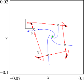
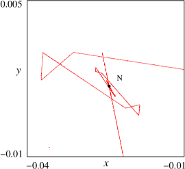
(a)               (b)

Figure 5: (a) Phase portrait of the attractor at $\tau_{R}=0.28$ with $\tau_{L}=-0.3$, $\delta_{L}=-0.3$, $\delta_{R}=1.4$ and $\mu=0.05$. (b) Magnified part of the IC marked by the square in (a) displays the loops on IC.

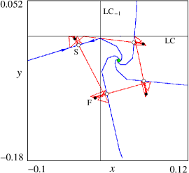
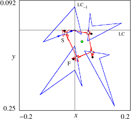
(a)               (b)

Figure 6: Phase portraits of the attractors at (a) $\tau_{R}=0.4$ and (b) $\tau_{R}=0.4295$ with other parameters same as in Fig. 3.

Let us now characterize the mechanism of occurrence of chaos in detail. The phase portrait at $\tau_{R}=0.25$ is shown in Fig. 3(a). The period-$4$ attracting cycle has real eigenvalues. The period-$4$ saddle cycle always has one positive eigenvalue $\lambda_{1}>1$ and another eigenvalue $-1<\lambda_{2}<0$. Since the stable eigenvalue of the saddle cycle is negative, so our map is orientation reversing and hence upon successive iterations, points on the stable manifold oscillate about the saddle point as they approaches to it. The closed invariant curve is formed by the union of the unstable manifolds of period-$4$ flip saddle cycle and the points of the period-$4$ regular attractor and flip saddle cycles. It is non-smooth, since the unstable manifolds are as smooth as the original map and our map is piecewise smooth. This curve forms the mode-locked torus. Fig. 3(a) shows that the unstable manifolds are self-intersecting. As our map is an endomorphism, the unstable manifold of a saddle point can intersect itself as well as the unstable manifold of another saddle point of the same saddle cycle. At $\tau_{R}=0.25$ the unstable manifold of a saddle point intersects the unstable manifold of another saddle point of the same period-$4$ saddle cycle (see Fig. 3(b)). Both types of self-intersections appear at $\tau_{R}\approx 0.28$ (see Fig. 5(a)). Since our map is non-invertible, a point on the unstable manifold can have two distinct preimages so the unstable manifolds are self-intersecting, though they are connected. From the definition of unstable manifold, we can say that there are infinite number of self-intersections (for both types) because the image of a self-intersecting point is again a self-intersecting point. With increase of the parameter, at $\tau_{R}\approx 0.28$ loops are created on the invariant curve (see Fig. 5(a)). Since at the points of self-intersections (first type) loops are developed so the infinite loop structure is formed on the invariant curve (see Fig. 5(b)). The torus formed by this invariant curve is a loop torus V. Maistrenko et al. (2003). As the parameter is increased to $\tau_{R}\approx 0.2855$, the eigenvalues of the stable cycle become complex conjugate. Then the closed invariant curve is formed by the union of the unstable manifolds of period-$4$ flip saddle cycle and the points of the period-$4$ spiral attractor and flip saddle cycles. Again increasing $\tau_{R}$, the unstable manifolds of the period-$4$ flip saddle cycle nontransversally touch the stable manifolds of it. Then the first homoclinic tangency appears at $\tau_{R}\approx 0.4$ (see Fig. 6(a)). Since the stable eigenvalue of the saddle cycle is negative, the homoclinic orbit flips around the saddle point. Thus the homoclinic tangency occurs in both sides of the stable manifold. With further increase of $\tau_{R}$, the stable and unstable manifolds of the period-$4$ flip saddle cycle intersect transversally to form a homoclinic tangle (see Fig. 6(b)). The existence of homoclinic tangle gives rise to Smale horseshoe dynamics, consequently an infinite number of high periodic orbits are created. The torus no longer exists, but the period-$4$ spiral attractor and the flip saddle cycle persist. Further increasing $\tau_{R}$, the second homoclinic tangency occurs at $\tau^{h}_{R}\approx 0.5$ (see Fig. 7(a)). The period-$4$ spiral attractor coexists with a chaotic attractor between the parameter values $\tau^{h}_{R}$ and $\tau^{c}_{R}$. At $\tau^{c}_{R}\approx 0.57414$ the period-$4$ spiral attractor and flip saddle cycles merge and disappear through border collision fold (saddle-focus) bifurcation.

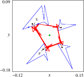
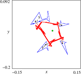
(a)               (b)

Figure 7: Attractors are depicted at (a) $\tau_{R}=0.5$ and (b) $\tau_{R}=0.53$ with other parameters same as in Fig. 3.

This scenario of transition to chaos is quite different from that in invertible maps since the self-intersections of the unstable manifolds and creation of loops on the invariant curve are impossible in invertible maps D. G. Aronson et al. (1982); Z. T. Zhusubaliyev et al. (2008a). There is only one attractor before the first homoclinic tangency, namely, the closed invariant curve consisting of the periodic orbits. After the appearance of the homoclinic tangle, the closed invariant curve is destroyed, yet the period-$4$ spiral attractor continues to exist. The stable manifold of the saddle point to the left side of the border ($x=0$) touches the critical curve LC at $\tau_{R}\approx 0.4295$ (see Fig. 6(b)). Then a contact bifurcation C. Mira et al. (1996) occurs. It causes changes in the basin of attraction of the period-$4$ spiral attractor, simply connected to nonconnected and unbounded to bounded, since the basin boundary is formed by the stable manifolds of the saddle cycle. A different basin of attraction for the period-$4$ attractor is created. The stable manifolds of each of the four saddle points are disconnected from each other. The stable manifold of a non-invertible map can intersect itself when the map is structurally unstable. Owing to the presence of the homoclinic tangle, our map has already become structurally unstable. So the stable manifolds of the period-$4$ flip saddle cycle form nonconnected (with finite number of simply connected components) and bounded basin of attraction of the period-$4$ spiral attractor. To our knowledge, this phenomenon in PWS dynamics has not been reported earlier. The stable manifolds fold at every intersection with the $y$-axis S. Banerjee and C. Grebogi (1999). Other fold points on the stable manifolds are preimages of the fold points on the $y$-axis in $Z_{2}$. As we increase $\tau_{R}$, the size of the basin of attraction of the period-$4$ spiral attractor diminishes (see Fig. 7(b)). This size tends to zero just before the border collision fold bifurcation.

VI Conclusion

The study of non-invertible dynamical systems is an important and recently flourishing research subject. In contrast to the earlier investigations S. Banerjee and C. Grebogi (1999); Z. T. Zhusubaliyev et al. (2006); Z. T. Zhusubaliyev et al. (2008a, b), here we have chosen the situation where the map (1) is non-invertible, and the determinant of the Jacobian matrix in one side of the bifurcation point is less than unity and is greater than unity in the other side. Such a situation arises in many physical systems like power electronic circuits. In this paper we have illustrated a scenario of transition from phase-locked dynamics to chaos in such a non-invertible piecewise smooth map. The closed invariant curve is formed by the union of the unstable manifolds of a saddle cycle and the points of stable and saddle cycles. Since a point can have two distinct preimages, the unstable manifolds have structurally stable self-intersections. We have found that loops are created on the invariant curve although there is no chance of appearance of cusps on it. As our map is linear in both sides of the border and the critical curve is the $x$-axis which has no cusp point, so cusps do not appear on the invariant curve. Here the invariant curve is destroyed through a homoclinic bifurcation. We have shown that contact bifurcation occurs when the stable manifold touches the critical curve. This bifurcation causes a qualitative change in the structure of basin of attraction, from simply connected and unbounded to nonconnected and bounded. At that point, the stable manifolds are self-intersecting since the system has become structurally unstable after the appearance of homoclinic tangle. We have observed the hysteretic transitions between mode-locked dynamics to chaotic dynamics and vice versa and have found the mechanism to be quite different from that in invertible maps.

References

- S. Banerjee and G. C. Verghese (2001) S. Banerjee and G. C. Verghese, eds., Nonlinear Phenomena in Power Electronics: Attractors, Bifurcations, Chaos, and Nonlinear Control (IEEE Press, New York, USA, 2001).
- Z. T. Zhusubaliyev and E. Mosekilde (2003) Z. T. Zhusubaliyev and E. Mosekilde, Bifurcations and Chaos in Piecewise-Smooth Dynamical Systems (World Scientific, Singapur, 2003).
- M. di Bernardo et al. (2007) M. di Bernardo, C. J. Budd, A. R. Champneys, and P. Kowalczyk, Piecewise-smooth Dynamical Systems: Theory and Applications (Applied Mathematical Sciences), vol. 163 (Springer-Verlag, London, 2007).
- S. Banerjee and C. Grebogi (1999) S. Banerjee and C. Grebogi, Physical Review E 59, 4052 (1999).
- B.Brogliato (1999) B.Brogliato, Nonsmooth Mechanics—Models, Dynamics and Control (New York: Springer Verlag, 1999).
- J. Ing et al. (2008) J. Ing, E. Pavlovskaia, M. Wiercigroch, and S. Banerjee, Philosophical Transactions of the Royal Society A 366, 679 (2008).
- J. Laugesen and E. Mosekilde (2006) J. Laugesen and E. Mosekilde, Comput. Oper. Res. 33, 464 (2006).
- C. M. Berger et al. (2007) C. M. Berger, X. Zhao, D. G. Schaeffer, H. M. Dobrovolny, W. Krassowska, and D. J. Gauthier, Physical Review Letters 99, 058101 (2007).
- H. E. Nusse and J. A. Yorke (1992) H. E. Nusse and J. A. Yorke, Physica D 57, 39 (1992).
- H. E. Nusse et al. (1994) H. E. Nusse, E. Ott, and J. A. Yorke, Physical Review E 49, 1073 (1994).
- M. di Bernardo et al. (1999) M. di Bernardo, M. I. Feigin, S. J. Hogan, and M. E. Homer, Chaos, Solitons & Fractals 10, 1881 (1999).
- P. Kowalczyk (2005) P. Kowalczyk, Nonlinearity 18, 485 (2005).
- M. Dutta et al. (1999) M. Dutta, H. E. Nusse, E. Ott, J. A. Yorke, and G-H. Yuan, Physical Review Letters 83, 4281 (1999).
- Hassouneh et al. (2004) M. A. Hassouneh, E. H. Abed, and H. E. Nusse, Phys. Rev. Lett. 92, 070201 (2004).
- Z. T. Zhusubaliyev et al. (2006) Z. T. Zhusubaliyev, E. Mosekilde, S. Maity, S. Mohanan, and S. Banerjee, Chaos 16, 11 (2006).
- Z. T. Zhusubaliyev et al. (2008a) Z. T. Zhusubaliyev, E. Mosekilde, S. De, and S. Banerjee, Physical Review E 77, 026206 (2008a).
- Z. T. Zhusubaliyev et al. (2008b) Z. T. Zhusubaliyev, E. Mosekilde, and S. Banerjee, Int. J. Bifurcation and Chaos 18, 1775 (2008b).
- V. S. Afraimovich and L. P. Shilnikov (1991) V. S. Afraimovich and L. P. Shilnikov, American Mathematical Society Translations 149, 201 (1991).
- D. G. Aronson et al. (1982) D. G. Aronson, M.A. Chory, G.R. Hall, and R.P. McGehee, Communications in Mathematical Physics 83, 303 (1982).
- V. Maistrenko et al. (2003) V. Maistrenko, Yu. Maistrenko, and E. Mosekilde, Physical Review E 67, 046215 (2003).
- E. N. Lorenz (1989) E. N. Lorenz, Physica D 35, 299 (1989).
- C. E. Frouzakis et al. (2003) C. E. Frouzakis, I. G. Kevrekidis, and B. B. Peckham, Physica D 177, 101 (2003).
- C. Mira et al. (1996) C. Mira, L. Gardini, A. Barugola, and J. C. Cathala, Chaotic Dynamics in Two-dimensional Noninvertible Maps (World Scientific, Singapore, 1996).
- Yang Wei-ming and Hao Bai-lin (1987) Yang Wei-ming and Hao Bai-lin, Communications in Theoretical Physics 8, 1 (1987).
- Z. T. Zhusubaliyev et al. (2002) Z. T. Zhusubaliyev, E. A. Soukhoterin, and E. Mosekilde, Chaos, Solitons & Fractrals 13, 1889 (2002).
- D. J. W. Simpson and J. D. Meiss (2008) D. J. W. Simpson and J. D. Meiss, SIAM Journal on Applied Dynamical Systems 7, 795 (2008).
- C. Robinson (1999) C. Robinson, Dynamical Systems - Stability, Symbolic Dynamics, and Chaos (CRS Press, 2nd edition, 1999).
- C. E. Frouzakis et al. (1997) C. E. Frouzakis, L. Gardini, I. G. Kevrekidis, and G. Millerioux, Int. J. Bifurcation and Chaos 7, 1167 (1997).