Quantum instability in a dc-SQUID with strongly asymmetric dynamical parameters

Abstract

A classical system cannot escape out of a metastable state at zero temperature. However, a composite system made from both classical and quantum degrees of freedom may drag itself out of the metastable state by a sequential process. The sequence starts with the tunneling of the quantum component which then triggers a distortion of the trapping potential holding the classical part. Provided this distortion is large enough to turn the metastable state into an unstable one, the classical component can escape. This process reminds of the famous baron Münchhausen who told the story of rescuing himself from sinking in a swamp by pulling himself up by his own hair—we thus term this decay the ‘Münchhausen effect’. We show that such a composite system can be conveniently studied and implemented in a dc-SQUID featuring asymmetric dynamical parameters. We determine the dynamical phase diagram of this system for various choices of junction parameters and system preparations.

I Introduction

Consider a classical object (a degree of freedom) trapped in a metastable potential minimum; no decay out of this metastable state is possible at low temperatures, where thermal activation over the barrier is exponentially suppressed. However, if the classical object is a composite one, with a quantum degree of freedom coupled to the classical one, then the quantum object may tunnel out of the metastable minimum and exert a pulling force on the classical object. Once the latter is large enough to completely suppress the trapping barrier, the classical object is able to leave the potential well—hence a classical object may escape from a metastable state even at zero temperature if helped by a coupled quantum degree of freedom.

The above situation can be realized in a dc-SQUID (Superconducting Quantum Interference Device) featuring asymmetric dynamical parameters; i.e., with two Josephson junctions of equal critical currents $J_{\mathrm{c}}$ but strongly different (shunt) capacitances $C$ and (shunt) resistances $R$, see Fig. 1; choosing large and small parameters $C$ and $1/R$ for the two junctions allows to place one of the junctions in the ‘classical’ and the other into the quantum domain. The tunneling of the quantum degree of freedom entails a distortion of the trapping potential of the classical junction, which might be sufficiently large to transform the metastable state of the classical junction into an unstable one. The appearance of this complex decay channel depends critically on the applied bias current $J$ and the SQUID’s loop inductance $L$ coupling the two junctions.

Figure 1: Schematics of the dynamically asymmetric dc-SQUID. Two Josephson junctions are integrated in a current ($J$) biased superconducting loop with inductance $L$. The two junctions feature equal critical currents $J_{\mathrm{c}}$ but strongly asymmetric (shunt) capacitances $C_{i}$ and (shunt) resistances $R_{i}$. We assume that $C_{i}$ and $R_{i}$ are chosen such that quantum effects are present for junction 2 but are strongly suppressed for junction 1, hence $C_{1}\gg C_{2}$ and/or $R_{1}\ll R_{2}$.

The gauge invariant phase differences $\varphi_{i}$, $i=1,2$, across the two Josephson junctionsJosephson:1962 define our dynamical degrees of freedom: Assuming equal critical currents $J_{c}$, the junctions’ potential energies ${\cal V}_{i}=E_{J}[1-\cos\varphi_{i}]$, $i=1,2$, involve the Josephson energy $E_{J}=\Phi_{0}J_{c}/2\pi c$ (with $\Phi_{0}=hc/2e$ the flux unit, $e$ and $c$ denote the unit charge and light velocity).footnote1 Their kinetic energies ${\cal T}_{i}=(\hbar/2e)^{2}C_{i}\dot{\varphi}_{i}^{2}/2$ are determined by the junction capacitances $C_{i}$ playing the role of effective masses (the relevant energy scale is given by the charging energy $E_{c,i}=e^{2}/2C_{i}$)—a dynamically asymmetric SQUID with one large and one small junction capacitance then provides us with the desired classical and quantum degrees of freedom (we choose $C_{1}\gg C_{2}$; additional normal resistances $R_{i}$ introduce a dissipative dynamical component, see below). The coupling of the two junctions via the loop inductance $L$ produces the interaction energy ${\cal V}_{\mathrm{int}}=[(\Phi_{0}/2\pi)^{2}/2L](\varphi_{2}-\varphi_{1})^{2}$ involving the relative coordinate $(\varphi_{2}-\varphi_{1})$, whereas the external driving current $J$ couples to the absolute coordinate, ${\cal V}_{\rm drive}=E_{J}(J/2J_{c})(\varphi_{1}+\varphi_{2})$. While large-capacitance (‘classical’) junctions are easily fabricated, small (‘quantum’) junctions are more difficult to realize. Nevertheless, experimental techniques to fabricate small junctions are available today and their quantum behavior in the form of quantum tunneling, Voss:1981 ; Caldeira:1981 ; Caldeira:1983 ; Devoret:1985 quantized energy levels Martinis:1985 ; Martinis:1987 and even quantum coherence Chakravarty:1984 ; Leggett:1987 ; Nakamura:1997 ; Nakamura:1999 ; Friedman:2000 ; Wal:2000 ; Chiorescu:2003 has been demonstrated.

The quantum decay of the biased, dynamically symmetric dc-SQUID has been discussed before both experimentallyLi:2002 ; Balestro:2003 and theoretically,Chen:1986 also in the context of instanton splitting.Ivlev:1987 ; Morais-Smith:1994 In the SQUID discussed here, footnote2 the large asymmetry of the dynamical parameters blocks the tunneling of the $\varphi_{1}$ degree of freedom; the ‘heavy’ junction then remains frozen during the quantum decay of the ‘light’ degree of freedom $\varphi_{2}$. A trajectory of this kind describes the entry of flux into the SQUID loop which rearranges the current flow in the two arms in a way as to redirect more current through the heavy junction. This increase in current produces an enhanced tilt $-J_{\mathrm{eff}}\varphi_{1}$ in the potential of the heavy junction, which then may decay through a classical trajectory, see Fig. 2. We call this nontrivial decay sequence the ‘Münchhausen decay’. It is the aim of this work to determine the effective critical current $J_{c}(L^{-1})$ for which the Münchhausen decay becomes possible, see Figs. 5 and 9-12.

In the following, we define our system in full detail, including a dissipative component in the junction dynamics (Sec. II). Sections III and IV are devoted to the derivation of the effective critical currents for the various cases with junctions governed by massive or dissipative dynamics. In Section V we add remarks concerning the experimental realization of the system described here. Finally, we draw conclusions in Section VI.

II Setup and model

Within the resistively and capacitively shunted junction (RCSJ) model (at $T=0$), the classical dynamics of the two phase differences $\varphi_{1}$ and $\varphi_{2}$ is governed by the equations of motion

$$\omega_{0,i}^{-2}\ddot{\varphi}_{i}+\eta_{i}\dot{\varphi}_{i}=-\partial_{\varphi_{i}}v(\varphi_{1},\varphi_{2}),$$ (1)

with the plasma frequency $\hbar^{2}\omega_{0,i}^{2}=8E_{J}E_{c,i}$ of an unbiased single junction and the damping coefficients $\eta_{i}=\Phi_{0}/2\pi cJ_{c}R_{i}$ ($R_{i}$ denote the normal ohmic junction resistances). The potential (see Fig. 2) is given by

$$v(\varphi_{1},\varphi_{2})=1-\cos\varphi_{1}+1-\cos\varphi_{2}\\ -j(\varphi_{1}+\varphi_{2})+\frac{k}{2}(\varphi_{1}-\varphi_{2})^{2},$$ (2)

with the dimensionless current $j=J/2J_{c}$ and the coupling constant $k=\Phi_{0}c/2\pi J_{c}L=1/\beta_{L}$ ($\beta_{L}$ denotes the usual screening parameter of the SQUID). Eqns. (1) and (2) describe a dc-SQUID with symmetric inductance $L$ in a vanishing external magnetic field and driven by a bias current $J$ or, equivalently, the massive (mass $\propto\omega_{0,i}^{-2}$) and/or dissipative ($\eta_{i}$) dynamics of two harmonically ($k$) coupled particles in a tilted ($j$) and corrugated ($\cos\varphi_{i}$) potential. Quantum effects of the light junction 2 are accounted for via the relevant tunneling and decay processes, see below.

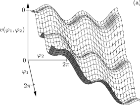
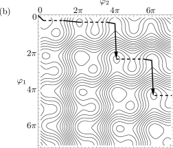
Figure 2: Surface (a) and contour plot (b) of the SQUID potential, Eq. (2), at bias current $j=0.5$ and coupling $k=0.04$. For an undercritical current $j<1$, the symmetric minima $(\varphi_{1}=\varphi_{2})$ are all metastable. The stability of the side-minima $(\varphi_{1}\neq\varphi_{2})$ depends crucially on the parameters $j$ and $k$. The line in (b) shows the decay path in an overdamped setup: The system starts out in a relaxed local ground state near the initial minimum at $\varphi_{1}=\varphi_{2}=\arcsin j$. The ‘light’ degree of freedom $\varphi_{2}$ then tunnels (dotted line) and the system relaxes to the bottom of the next minimum near $\varphi_{2}\approx 2\pi$, with a classically stable but quantum mechanically metastable ground state. Through an additional quantum phase slip, the light phase reaches the minimum near $\varphi_{2}\approx 4\pi$, which is not classically stable and henceforth the system can decay along a classically allowed path to $\varphi_{1}\approx 2\pi$. The system then has turned unstable and enters a resistive state through iteration of the last two steps.

The potential (2) gives rise to two types of relevant frequencies. One is the plasma frequency $\omega_{p,i}$, the small-amplitude frequency in the direction of $\varphi_{i}$ around a local minimum of the potential $v(\varphi_{1},\varphi_{2})$. With the effective potential

$$v_{\mathrm{eff}}[\varphi_{l}](\varphi_{i})=v(\varphi_{l}=\mathrm{const.},\varphi_{i}),\ i\neq l,$$ (3)

cf. Fig. 3, $\omega_{p,i}^{2}=\omega_{0,i}^{2}\partial_{\varphi_{i}}^{2}v_{\mathrm{eff}}(\varphi_{i})$, evaluated at a local minimum $\varphi_{i}^{\mathrm{min}}$, and depends on the parameters $j$ and $k$ as well as on $\varphi_{i}^{\mathrm{min}}$. For the heavy junction (junction 1), $\omega_{p,1}$ can become arbitrarily small upon approaching criticality, while for the quantum junction (junction 2) $\omega_{p,2}$ becomes small only for $j\rightarrow 1$ and $k\to 0$. The other frequency is given by the $LC$ constant of the ‘superwell’ in $v_{\mathrm{eff}}(\varphi_{2})$, cf. Fig. 3, and is relevant only in the regime $k\ll 1$ and for the quantum junction (junction 2), $\omega_{\mathrm{LC,2}}^{2}=\omega_{0,2}^{2}k=c^{2}/LC_{2}$.

Figure 3: Effective potential $v_{\mathrm{eff}}(\varphi_{2})=v(\varphi_{1}=\mathrm{const.},\varphi_{2})$ (solid line) and the parabola remaining after dropping $\cos\varphi_{2}$ (dashed line) for $j=0.5$, $k=0.02$ and $\varphi_{1}=\arcsin j$. The bullets and arrows illustrate the sequential decay of the quantum phase $\varphi_{2}$ to the ground state for the case of strong damping.

These characteristic frequencies delineate the regimes where the two junctions behave classically and quantum mechanically, respectively. The relevant physical parameters are given by the ratios $E_{J}/E_{c,i}$. For the heavy junction, we have to make sure that the number $N_{l}\approx E_{b}/\hbar\omega_{p,1}\sim(E_{J}/E_{c,1})(1-J_{1}/J_{c})^{5/4}$ of states in the local well remains large. Choosing a large ratio $E_{J}/E_{c,1}\gg 1$ then guarantees that quantum effects (i.e., $N_{l}$ of order unity) become relevant only very close to criticality and we choose to ignore them in our discussion below.

The system develops the most interesting behavior if the quantum degree of freedom develops well localized states within all relevant local minima in $v_{\mathrm{eff}}(\varphi_{2})$, Fig. 3, and hence parameters should be chosen such that the quasi-classical description applies. On the other hand, we require tunneling and coherence effects to manifest themselves on reasonably short (measurable) timescales. We then choose a ratio $E_{J}/\hbar\omega_{0,2}\sim 2$, such that the local wells in $v_{\mathrm{eff}}(\varphi_{2})$ contain a few quasi-classical states each.

The strength of dissipation can be quantified by the dimensionless damping parameters,

$$\alpha_{p,i} = (2R_{i}C_{i}\omega_{p,i})^{-1},$$ (4)

$$\alpha_{LC,2} = (2R_{2}C_{2}\omega_{LC,2})^{-1}.$$ (5)

Below, we are interested in the two limiting cases of strong and weak damping. For a strongly damped quantum junction with $\alpha_{p,2}>1$, the quantum decay of $\varphi_{2}$ out of a metastable well of $v_{\mathrm{eff}}(\varphi_{2})$ is incoherent Caldeira:1983 ; Leggett:1987 and its subsequent relaxation is fast (as compared to the dynamics of $\varphi_{1}$). For weak damping, $\alpha_{LC,2}\ll 1$, $\alpha_{p,i}\ll 1$, the kinetic energy stored in the motion of the heavy junction has to be accounted for; in addition, the finite lifetime of the quantum states of the light junction due to the residual dissipation has to be considered, see the discussion in Sec. IV.

III Strong damping

We start by analyzing the situation for strong damping, $\alpha_{p,2}>1$ and $\alpha_{p,1}\gg 1$, see Ref. Thomann:2008, for an earlier short report. We bear in mind an experiment with a dc-SQUID characterized by a fixed inductance $L\propto k^{-1}$ and biased with a current $j<1$. The task is to determine whether the Münchhausen decay can take place; in the experiment, the latter manifests itself through the transition to a finite voltage state. In the strong damping case, no kinetic energy is stored in the system. Furthermore, the evolution is not sensitive to the way the current is ramped. After current ramping, the system starts out in a relaxed state where the phases $\varphi_{i}$ are localized in the diagonal metastable minimum at $\varphi_{1}=\varphi_{2}=\arcsin j$ (up to an arbitrary multiple of $2\pi$).

For sufficiently large $j$, the quantum degree of freedom $\varphi_{2}$ undergoes tunneling to a new local minimum nearby $2\pi n$, while the classical degree of freedom $\varphi_{1}=\arcsin j$ remains localized, thus allowing a flux $\simeq n\Phi_{0},\ n\in\mathbb{N}$ to enter the SQUID loop, cf. Fig. 3. If the resulting force on the classical phase $\varphi_{1}$ is sufficiently large, the Münchhausen decay is enabled with a classical decay of $\varphi_{1}$ and successive iteration of quantum decay (directed along $\varphi_{2}$, flux entry) and classical relaxation (directed mainly along $\varphi_{1}$, flux exit), cf. Fig. 2.

Figure 4: Illustration of the assembly of $j_{c}(k)$ from the segments $j_{c,1}^{+}(k)$, Eq. (6), and $j_{c,1}^{-}(k)$, Eq. (11). In (c), the relevant region of the $j$-$k$-plane is shown. At A, the quantum junction (see (b)) has relaxed to the initial minimum ($n=0$) and the classical junction is localized in a stable minimum (see (a)). Increasing the bias current $j$ and approaching B, the potential barrier confining the classical phase in $v_{\mathrm{eff}}(\varphi_{1})$ is only slightly reduced. As $j>j_{c,1}^{+}(k)$ (C), the increase in $j$ has deformed the effective potential $v_{\mathrm{eff}}(\varphi_{2})$ as to allow a phase slip of $\varphi_{2}$ (see (b)). The additional force it exerts on the classical junction immediately removes the barrier (see (a)) and delocalizes $\varphi_{1}$ at $j_{c}(k)=j_{c,1}^{+}(k)$. On the other hand, an increase in bias $j>j_{c,1}^{+}(k)$ from A^′ to B^′ at lower $k$ leads to a phase slip of $\varphi_{2}$ (see (e)), without delocalizing $\varphi_{1}$ (see (d)). A further increase in $j$ triggers a classical decay (see (d)) when crossing the critical line at $j_{c}(k)=j_{c,1}^{-}(k)$ (C^′).

The strong coupling at large $k$ keeps the local minimum at $\varphi_{2}=\arcsin j$ lower in energy than the adjacent local well at $\varphi_{2}\approx 2\pi$ for all bias currents $j$, hence tunneling is inhibited and no Münchhausen decay takes place. At lower $k$, a bias current $j<1$ can sufficiently lower the adjacent well such as to bring both minima to equal height. This condition is reached once the minimum of the parabola in $v_{\mathrm{eff}}(\varphi_{2})$ (at $\varphi_{2}=\arcsin j+j/k$) is aligned with the midpoint between the two corresponding minima of $-\cos\varphi_{2}$ (at $\varphi_{2}=\pi$); i.e., if $\arcsin j+j/k=\pi$. Thus, for $k<k_{c,1}^{+}(j)$ withhallatschek:2000

$$k_{c,1}^{+}(j)=\frac{j}{\pi-\arcsin j},$$ (6)

the minimum at $\varphi_{2}\approx 2\pi$ is lower and a quantum decay is enabled (cf. Fig. 4(b), point C in the diagram). The jump of $\varphi_{2}$ by roughly $2\pi$ then pulls the heavy junction out of its minimum and the Münchhausen decay is initiated, cf. Figs. 4(a) and (b) associated with the sequence of points A, B, and C in Fig. 4(c). The smaller $k$ becomes, i.e., the weaker $\varphi_{2}$ is bound to $\varphi_{1}$, the less current is needed to lower the adjacent minimum such as to allow for a decay of $\varphi_{2}$, hence the positive slope of $k_{c,1}^{+}(j)$.

Decreasing $k$ too far, however, the pulling force exerted by the quantum junction may not be sufficient to drag the heavy junction out of its minimum. Hence, we have to investigate the shape of the potential $v(\varphi_{1},\varphi_{2})$ after the phase slip in $\varphi_{2}$, i.e., nearby the point $\varphi_{1}\gtrsim\arcsin j,\ \varphi_{2}\approx 2\pi$, and check whether the barrier against a classical decay (mainly along $\varphi_{1}$) has disappeared; this is identical to the calculation of the critical current of a SQUID with a trapped flux.Tsang:1975 ; Lefevre-Seguin:1992

We first determine the position of the minimum by solving the equations

$$\partial_{\varphi_{1}}v(\varphi_{1},\varphi_{2}) = \sin(\varphi_{1})-j+k(\varphi_{1}-\varphi_{2})=0,$$ (7)

$$\partial_{\varphi_{2}}v(\varphi_{1},\varphi_{2}) = \sin(\varphi_{2})-j-k(\varphi_{1}-\varphi_{2})=0,$$ (8)

for $\varphi_{1}\gtrsim\arcsin j$ and $\varphi_{2}\approx 2\pi$. At the critical coupling $k_{c,1}^{-}(j)$ the minimum should merge with a saddle and define an inflection point along some direction in the $(\varphi_{1},\varphi_{2})$-plane. The resulting system of equations requires numerical solution and the result is shown in the inset of Fig. 5. However, within the interesting region at small coupling $k$ we can find an approximate analytical solution: For $k\ll 1$, the side minimum of $v(\varphi_{1},\varphi_{2})$ becomes unstable predominantly along the $\varphi_{1}$-direction. Thus, the minimum disappears if

$$\partial_{\varphi_{1}}^{2}v(\varphi_{1},\varphi_{2})=\cos\varphi_{1}+k=0.$$ (9)

We choose the solution $\varphi_{1}\approx\pi/2$ (we set $k=0$ and assume $0\leq\varphi_{1}<2\pi$; the other solution $\varphi_{1}\approx 3\pi/2$ cannot solve Eq. (7) and is discarded). Inserting $\varphi_{1}$ into the sum of Eqs. (7) and (8) yields the relation

$$\sin\varphi_{2}\approx 2j-1,$$ (10)

from which we find $\varphi_{2}\approx 2\pi+\arcsin[2j-1]$ (the other solution $\varphi_{2}\approx 3\pi-\arcsin[2j-1]$ is excluded since it describes a maximum along the $\varphi_{2}$-direction). Inserting $\varphi_{1}$ and $\varphi_{2}$ into Eq. (7), we find the condition

$$k_{c,1}^{-}(j)\approx\frac{1-j}{(3/2)\pi+\arcsin(2j-1)}.$$ (11)

For $k>k_{c,1}^{-}(j)$ no barrier blocks the motion of $\varphi_{1}$ after the phase slip in $\varphi_{2}$ and a classical decay of $\varphi_{1}$ is enabled, thus completing the Münchhausen decay. This scenario is described by the sequence A, B, C in Fig. 4(c). For $k<k_{c,1}^{-}(j)$ the force after the phase slips is too small and an additional increase in $j$ is necessary to drive the system overcritical, as illustrated by the sequence A^′, B^′, C^′ in Fig. 4(c) and Figs. 4(d) and (e). The increase in critical current with decreasing coupling defines a negative slope for $k_{c,1}^{-}(j)$.

We define the effective critical current $j_{c}(k)$ as the phase boundary between the stable region ($j<j_{c}(k)$), where the Münchhausen decay is prohibited, and the delocalized phase ($j>j_{c}(k)$). This critical line is assembled from the segments $j_{c,1}^{\pm}(k)$, the inverse functions of $k_{c,1}^{\pm}(j)$, Eqs. (6) and (11), respectively: Ramping up the current $j$ at large values of $k$, we eventually cross $j_{c,1}^{+}(k)$. The phase slip of $\varphi_{2}$ immediately enables the classical decay of $\varphi_{1}$ and the system enters a running state, hence, $j_{c}(k)=j_{c,1}^{+}(k)$. At lower $k$, increasing $j$ beyond $j_{c,1}^{+}(k)$ triggers a phase slip of $\varphi_{2}$, but the resulting force is too weak to delocalize $\varphi_{1}$. A further increase in $j$ is necessary until, at $j=j_{c,1}^{-}(k)$, the minimum disappears and the Münchhausen decay proceeds, hence, $j_{c}(k)=j_{c,1}^{-}(k)$.

Following the above discussion, the system is stable for $j<j_{c,1}^{-}(k)$. Upon further decreasing $k$, however, more and more side minima in $v_{\mathrm{eff}}(\varphi_{2})$ become accessible to the quantum junction. From Fig. 3 we notice, that the different local minima of $v_{\mathrm{eff}}(\varphi_{2})$ are located near $\varphi_{2}\approx 2\pi n$. They describe the state where a flux $\simeq n\Phi_{0}$ has entered the loop and we label them by the index $n$. Eq. (6) is then straightforwardly generalized to the critical line $k_{c,n}^{+}(j)$ describing the entry of the $n$-th fluxon. The $n$-th phase slip of $\varphi_{2}$ occurs when the global minimum in $v_{\mathrm{eff}}(\varphi_{2})$ shifts from $\varphi_{2}\approx 2\pi(n-1)$ to $\varphi_{2}\approx 2\pi n$. We can proceed analogously to the derivation of Eq. (6): Let $\varphi_{1}^{\mathrm{min},n-1}$ be the solution of Eqs. (7) and (8) near $\varphi_{1}\gtrsim\arcsin j,\ \varphi_{2}\approx 2\pi(n-1)$. In order to find the crossing in the height of the two minima we account for the relaxation of $\varphi_{1}$ and align the minimum of the shifted parabola ($\varphi_{2}=\varphi_{1}^{\mathrm{min},n-1}+j/k$) with the midpoint between the two minima of the $-\cos\varphi_{2}$-potential ($\varphi_{2}=(2n-1)\pi$), hence $\varphi_{1}^{\mathrm{min},n-1}+j/k=(2n-1)\pi$ and

$$k_{c,n}^{+}(j)=\frac{j}{(2n-1)\pi-\varphi_{1}^{\mathrm{min},n-1}}.$$ (12)

A convenient approximation is made by ignoring the relaxation of $\varphi_{1}$, resulting in the expression

$$k_{c,n}^{+}(j)\approx\frac{j}{(2n-1)\pi-\arcsin j}.$$ (13)

Similarly, we can generalize Eq. (11) to a critical coupling $k_{c,n}^{-}(j)$, determining whether the resulting force at given fluxon index $n$ is sufficient to delocalize $\varphi_{1}$. We then solve Eqs. (7) and (8) near $\varphi_{1}\approx\arcsin j,\ \varphi_{2}\approx 2\pi n$, proceed as in the derivation of Eq. (11), and find (for small $k\ll 1$)

$$k_{c,n}^{-}(j)\approx\frac{1-j}{(2n-1/2)\pi+\arcsin(2j-1)}.$$ (14)

Figure 5: Phase diagram of the dynamically asymmetric dc-SQUID as a function of bias current $j=J/2J_{c}$ and inductive coupling $k=\Phi_{0}c/2\pi LJ_{c}$. Here, we assume strong damping $\alpha_{p,1}\gg 1$ and $\alpha_{p,2}>1$. The effective critical current $j_{c}(k)$ (solid line) marks the boundary between a localized classical junction (lower bias $j<j_{c}$) and a delocalized classical junction ($j>j_{c}$), corresponding to a finite voltage state of the SQUID. Branches with negative slope are determined by a classical instability (mainly along $\varphi_{1}$), while those with positive slope are determined by a quantum instability of the light junction. For $j<j_{c}(k)$, the dotted lines $j_{c,n}^{+}(k)$ mark the entry of flux through the quantum junction (the integer $n$ approximately quantifies the flux through the ring in the stable state); these lines can be measured via monitoring of the flux threading the loop. For $j>j_{c}(k)$, the dashed lines $j_{c,m}^{-}(k)$ mark the minimum number $m$ of flux units necessary to delocalize the classical junction. The inset shows a comparison between the approximate result, Eqs. (13) and (14) (solid line) and the exact numerical result (dashed).

The critical current line $j_{c}(k)$ is constructed from interchanging segments of $j_{c,n}^{+}(k)$ and $j_{c,n}^{-}(k)$, resulting in the dynamical phase diagram, Fig. 5. Note that the different nature of the decay, classical or quantum, associated with the two types of critical lines may allow for an experimental distinction: Ramping the current past a ⁺-type segment of $j_{c}(k)$ triggers a quantum decay with a broad histogram describing multiple measurements. A ^--type segment of $j_{c}(k)$ triggers a classical decay with a sharp histogram (the quantum decay of $\varphi_{2}$ needs to have occurred already, which limits the ramping speed before reaching the critical line). Note that the lines $j_{c,n}^{+}(k)$ are detectable throughout all the stable portion of the phase diagram, e.g., via a measurement of the flux threading the loop (the flux increases by approximately one flux unit upon crossing the dotted lines in Fig. 5).

The phase diagram in Fig. 5 shows that the critical line $j_{c}(k)$ approaches the value $1/2$ for $k\rightarrow 0$. This is understood from analyzing Eqs. (13) and (14) for large $n$ and small $k$, providing the relations $k_{c,n}^{+}(j)\approx j/2n\pi$ and $k_{c,n}^{-}(j)\approx(1-j)/2n\pi$, respectively. Equating the two conditions gives $j_{c}\approx 0.5$. From a physical point of view, this result can be easily explained: The decay of $\varphi_{2}$ proceeds towards the bottom of the parabola in $v_{\mathrm{eff}}(\varphi_{2})$; for $k\rightarrow 0$, the current through the quantum junction then approaches zero, $J_{2}\propto\sin\varphi_{2}\approx 0$. Consequently, all current is redirected through the classical junction 1, with the effective bias now increased to $J_{1}=2jJ_{c}$. Junction 1 thus turns dissipative at $j=1/2$, the critical current of a single junction but half the critical current of the dc-SQUID.

Figure 6: Sketch of a time-trace of the flux threading the SQUID loop during the decay process of $\varphi_{1}$ and $\varphi_{2}$ at $j>j_{c}(k)$, cf. Fig. 2(b). The flux increases by approximately one flux unit each time the quantum junction decays; this process then involves the tunneling rate $\Gamma_{2}$ of $\varphi_{2}$, Eq. (15). The additional flux leaves the loop again within the time interval $\sim\eta_{1}$ as the classical junction relaxes dissipatively to the next minimum.

The dynamical phase diagram, Fig. 5, can be tested experimentally through a measurement of the dc-voltage drop across the device. The second Josephson relationJosephson:1962 tells that the time-averaged voltage $\langle V\rangle_{t}\propto\langle\dot{\varphi}_{1}\rangle_{t}=\langle\dot{\varphi}_{2}\rangle_{t}$. Inspecting Fig. 2(b), we understand that the continuous iteration of quantum and classical decays of the light and heavy phase variables generate the nonzero averages $\langle\dot{\varphi}_{1}\rangle_{t}=\langle\dot{\varphi}_{2}\rangle_{t}$ for $j>j_{c}(k)$. For the overdamped setup as described above, the voltage drop is small as strong damping reduces the tunneling rate determining $\langle\dot{\varphi}_{2}\rangle_{t}$. This is particularly true close to the critical line, where the variable $\varphi_{2}$ needs to tunnel in the ‘flat’ part of $v_{\mathrm{eff}}(\varphi_{2})$. The decay process is faster for weak damping and thus generates a larger voltage signal—we discuss this situation in the next Section.

Another characteristic signal of the Münchhausen decay is the time-trace of the magnetic flux threading the SQUID loop during the alternating decay of the two phases (cf. Fig. 2(b)), see Fig. 6 for an illustration. Such time-traces exhibit two characteristic time scales, one due to the tunneling of the quantum junction involving the rate $\Gamma_{2}$ separating subsequent peaks of flux entry into the loop; the other is due to the classical relaxation of the heavy junction and involves the dissipative time $\sim\eta_{1}$ describing the flux exit and return to the low-flux state of the loop. At small $k$ and small effective bias between two minima,

$$\frac{\Gamma_{2}^{(n)}}{\omega_{0,2}}\approx\frac{\hbar\omega_{0,2}E_{c,2}}{E_{J}^{2}}\left(\frac{R_{Q}}{\pi R_{2}}\right)^{7/2}(j-j_{c,n}^{+})^{2R_{Q}/R_{2}-1},$$ (15)

with $R_{Q}=h/4e^{2}$.korshunov:1987

IV Weak damping

The behavior of the system for weak damping $\alpha_{LC,2}\ll 1,\ \alpha_{p,i}\ll 1$ is quite similar to the one encountered before, while the (small) differences strongly depend on the many system parameters and their associated timescales. To begin with we neglect dissipative effects. Bearing in mind the limit of large $C_{1}/C_{2}$, we can exploit the adiabatic separation of fast and slow degrees of freedom; i.e., we first consider the fast problem for the quantum junction,

$$\mathcal{H}_{2}\Psi_{l}(\varphi_{2})=\varepsilon_{l}\Psi_{l}(\varphi_{2}),$$ (16)

with the reduced Hamiltonian (cf. Eq. (1))

$$\mathcal{H}_{2}=-4E_{c,2}\partial_{\varphi_{2}}^{2}+E_{J}v_{\mathrm{eff}}[\varphi_{1}](\varphi_{2})$$ (17)

defined at fixed $\varphi_{1}$. Eq. (16) establishes the dynamics of the ‘light’ variable $\varphi_{2}$ and we can find the energies $\varepsilon_{l}(\varphi_{1})$. These act as effective potentials for the ‘heavy’ degree of freedom $\varphi_{1}$; e.g., assuming the quantum junction to reside in a state $|l\rangle$, $\langle\varphi_{2}|l\rangle=\Psi_{l}(\varphi_{2})$, the effective potential for $\varphi_{1}$ is given by $\varepsilon_{l}(\varphi_{1})$. Typical examples for the effective potentials $\varepsilon_{0}(\varphi_{1})$ (ground state) and $\varepsilon_{1}(\varphi_{1})$ (first excited state) are shown in Fig. 7.

In the dissipative situation, we could derive the phase diagram from simply analyzing the potential $v(\varphi_{1},\varphi_{2})$; here, instead, we first determine which states $l$ of the light junction are relevant and then analyze the dynamics of $\varphi_{1}$ in the resulting effective potential (e.g., Fig. 7(a)) defined via $\varepsilon_{l}(\varphi_{1})$, thus determining whether the heavy junction stays localized or enters a running state. Both tasks strongly depend on the various timescales involved. We start with the timescale of the ‘external control’, the rate at which the bias $j$ is ramped. Whereas the case of strong damping excluded the presence of kinetic energy in the system, this is no longer the case here. The importance of the ramping rate then comes about through the amount of energy which is transferred to the two degrees of freedom. The change of $j$ translates to a change of the potential $v(\varphi_{1},\varphi_{2})$ with a rate of the order of $\partial_{t}j$. The ramping can be adiabatic, in which case no energy is given to the system, or instantaneous, where the amount of transferred energy is maximal. Intermediate types of ramping will not be discussed.

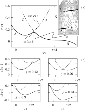
Figure 7: Illustration of the effective potential for the ‘heavy’ phase $\varphi_{1}$, generated by the two lowest levels of the ‘light’ phase. In (a), the situation for $k=0.15,\ j=0.36$ is shown. The avoided level crossing $2\Delta_{2}$ in the spectrum of the light junction is reflected in the effective potentials $\varepsilon_{0}(\varphi_{1})$ (solid) and $\varepsilon_{1}(\varphi_{1})$ (dotted) for the heavy junction. The inset illustrates the 2-dimensional path $[\varphi_{1},\varphi_{2}^{\mathrm{min},0/1}(\varphi_{1})]$ in $v(\varphi_{1},\varphi_{2})$ corresponding to $\varepsilon_{0}(\varphi_{1})$ (solid, A/B) and $\varepsilon_{1}(\varphi_{1})$ (dotted, C/D); the upward/downward jump along $\varphi_{2}$ to the next minimum corresponds to the avoided crossing in $\varepsilon(\varphi_{1})$. (b) Series of $\varepsilon_{0}(\varphi_{1})$ (solid) and $\varepsilon_{1}(\varphi_{1})$ (dotted) for various values of $j$ at $k=0.1$. Increasing $j$ shifts the position of the avoided crossing in $\varepsilon(\varphi_{1})$ to the left. Its transition past $\varphi_{1}^{\mathrm{min}}$ (between $j=0.26$ and $j=0.3$) corresponds to crossing the line $j_{c,1}^{+}(k)$ and implies the decay of the quantum junction to the next local minimum. Note that in the present case the newly formed minimum is stable (a point of type B^′ in Fig. 4).

The adiabatic separation of time scales requires a large capacitance ratio $C_{1}\gg C_{2}$. For $\omega_{p,1}\ll\omega_{p,2}$ the intravalley motion of the two junctions are separated. The (tunneling) motion of the light junction across valleys produces a stronger condition: Consider the tunneling splitting $\Delta_{2}$ in the spectrum of $\mathcal{H}_{2}$ at an avoided level crossing, cf. Fig. 7(a),

$$\Delta_{2}\sim\hbar\omega_{p,2}\exp\bigl{(}-\gamma\sqrt{{E_{J}}/{4E_{c,2}}}\bigr{)},$$ (18)

with $\gamma$ depending on the actual shape of the potential,

$$\gamma=\int_{a}^{b}d\varphi_{2}\sqrt{v_{\mathrm{eff}}(\varphi_{2})-E_{0}/E_{J}}$$ (19)

in the quasi-classical approximation. Here, $E_{0}$ is the ground state energy in the well and $a$ and $b$ are the left and right classical turning points, respectively, $v_{\mathrm{eff}}(\varphi_{2}=a)=v_{\mathrm{eff}}(b)=E_{0}/E_{J}$. The tunneling gap $\Delta_{2}$ then is relevant when analyzing the motion of the classical junction ($\varphi_{1}$) in the effective potential given by $\varepsilon_{l}(\varphi_{1})$. If the motion of $\varphi_{1}$ is sufficiently slow, its passage along an avoided crossing in the spectrum of $\mathcal{H}_{2}$ is adiabatic and $\varphi_{1}$ follows $\varepsilon_{l}(\varphi_{1})$ through the anticrossing (cf. the trajectory A$\,\to\,$B in Fig. 7(a)); i.e., the phase $\varphi_{2}$ tunnels to the next adjacent minimum. On the other hand, if the motion of $\varphi_{1}$ is fast, the state of the quantum junction undergoes Landau-Zener tunneling (cf. the trajectory A$\,\to\,$D in Fig. 7(a); the light junction then remains trapped in its local well) and $\varphi_{1}$ follows the effective potential $\varepsilon_{l\pm 1}(\varphi_{1})$ after the avoided crossing. The probability $p_{\mathrm{LZ}}$ for Landau-Zener tunneling at an anticrossing of the two lowest levels of $\mathcal{H}_{2}$ is given by

$$p_{\mathrm{LZ}}=\exp\left(-\frac{2\pi\Delta_{2}^{2}}{\hbar|d_{t}\varepsilon_{10}(t)|}\right),$$ (20)

where $\varepsilon_{10}(t)=\varepsilon_{1}(t)-\varepsilon_{0}(t)$ and $d_{t}$ is the total time derivative. To estimate the rate of change in energy $d_{t}\varepsilon_{10}(t)$, we start from

$$\varepsilon_{10}\approx E_{J}[v(\varphi_{1},\varphi_{2}^{\mathrm{min},n+1})-v(\varphi_{1},\varphi_{2}^{\mathrm{min},n})]$$ (21)

and find the time derivative

$$d_{t}\varepsilon_{10}(t) = \partial_{\varphi_{1}}\varepsilon_{10}\dot{\varphi}_{1}$$ (22)

$$+E_{J}\big{[}\partial_{\varphi_{2}}v(\varphi_{1},\varphi_{2})|_{\varphi_{2}^{\mathrm{min},n+1}}\partial_{\varphi_{1}}\varphi_{2}^{\mathrm{min},n+1}$$

$$-\partial_{\varphi_{2}}v(\varphi_{1},\varphi_{2})|_{\varphi_{2}^{\mathrm{min},n}}\partial_{\varphi_{1}}\varphi_{2}^{\mathrm{min},n}\big{]}\dot{\varphi}_{1}$$

$$= kE_{J}(\varphi_{2}^{\mathrm{min},n}-\varphi_{2}^{\mathrm{min},n+1})\dot{\varphi}_{1},$$

where we have used that $\partial_{\varphi_{2}}v(\varphi_{1},\varphi_{2})$ vanishes at the minima $\varphi_{2}^{\mathrm{min},n}$ and only the term originating from the coupling term in $v(\varphi_{1},\varphi_{2})$ is relevant. Since $\dot{\varphi}_{1}$ is at most of order $\omega_{0,1}$, we obtain the estimate $d_{t}\varepsilon_{10}\sim 2\pi k\omega_{0,1}E_{J}$. The smallness of $p_{LZ}$, guaranteeing adiabatic motion of the classical junction (this requires a correspondingly large $C_{1}$) then follows from

$$k\frac{E_{J}}{\Delta_{2}}\frac{\hbar\omega_{0,1}}{\Delta_{2}}\sim k\sqrt{\frac{E_{c_{1}}}{E_{c_{2}}}}\sqrt{\frac{E_{J}}{E_{c_{2}}}}\exp\Bigl{(}2\gamma\sqrt{\frac{E_{J}}{4E_{c_{2}}}}\Bigr{)}\ll 1.$$ (23)

The relaxation of the quantum degree of freedom $\varphi_{2}$ is another important element in our discussion. The dissipation described by the normal resistance $R$ in the RCSJ-equation of motion, cf. Eq. (1), leads to typical finite lifetimes $\tau_{2}\sim RC_{2}=1/2\alpha_{2}\omega_{p,2}$ of the excited states $|l\rangle$ of the quantum junction.esteve:1986 A much longer lifetime $\tilde{\tau}_{2}$ shows up if the quantum junction is trapped in a local ground state of a side-well in $v_{\mathrm{eff}}(\varphi_{2})$, cf. Fig. 8. The decay then is protected through a large barrier $E_{b}$, enhancing the typical lifetime to a value $\tilde{\tau}_{2}$, with $\tau_{2}\ll\tilde{\tau}_{2}\propto\exp(2\gamma\sqrt{E_{J}/4E_{c,2}})$.Averin:2000 Thus, there are two (extreme) ways how a highly exited state in the ‘superwell’ of $v_{\mathrm{eff}}(\varphi_{2})$ can decay, see Fig. 8, either via states within the superwell involving the typical lifetime $\tau_{2}$, or via states involving a tunneling process, resulting in an exponentially larger decay time of the order of $\tilde{\tau}_{2}$.

Figure 8: Illustration of decay sequences of an excited ‘superwell’-state of the quantum junction in the effective potential $v_{\mathrm{eff}}(\varphi_{2})$, Eq. (3). Solid arrows indicate a decay sequence involving only states within the ‘superwell’ with a typical decay time $\tau_{2}$. The dashed arrows illustrate another (extreme) decay sequence, involving localized states in the side-minima of $v_{\mathrm{eff}}(\varphi_{2})$. The decay time then involves the typical lifetime $\tilde{\tau}_{2}\gg\tau_{2}$ of local ground states within side-wells.

In the following, we investigate three regimes and derive the corresponding effective critical current $j_{c}(k)$. We begin with the case of adiabatic ramping (Sec. IV.1), where we assume that the ramping is slower than the typical relaxation time of the heavy junction and the timescales between $\varphi_{1}$ and $\varphi_{2}$ separate; i.e., inequality (23) holds. We show that the critical current $j_{c}(k)$ obtained in the dissipative case, Sec. III, is only slightly altered due to the (small) finite amount of kinetic energy the classical junction can store. Next, we discuss the case of fast ramping (Sec. IV.2), where the phase $\varphi_{1}$ remains effectively ‘frozen’ during the current ramping and quite an appreciable amount of potential energy is converted to kinetic energy in the motion of the classical junction, leading to a pronounced reduction of $j_{c}(k)$. Both discussions require a very large value of $C_{1}/C_{2}\rightarrow\infty$ to guarantee the absence of Landau-Zener tunneling due to the motion of $\varphi_{1}$. Subsequently, we discuss the consequences of a moderate ratio $C_{1}/C_{2}\lesssim 10^{4}$ accessible in today’s experiments in the last part of this section (Sec. IV.3). Then, $\varphi_{2}$ can remain trapped in a localized state in a side well during the motion and liberation of the heavy junction. The probabilistic effects emerging for this situation change the nature of the phase diagram qualitatively.

IV.1 Adiabatic ramping of the bias current

We start from the system with fixed coupling $k$ at $j=0$ and consider a state localized at $\varphi_{1}=\varphi_{2}=0$. We assume slow current ramping on the dissipative timescale of the classical junction’s motion,

$$\partial_{t}j\ll 1/\tau_{1},$$ (24)

where $\tau_{1}\sim RC_{1}$ denotes the classical relaxation time of the heavy junction. The inequalities (24) (slow ramping) and (23) (slow motion of $\varphi_{1}$) guarantee that the quantum junction remains in the global ground state, while the classical junction follows its local ground state near $\varphi_{1}=\arcsin j$.

The effective potential for the heavy junction then is determined by the ground state energy $\varepsilon_{0}(\varphi_{1})$. In our estimate

$$\varepsilon_{0}(\varphi_{1})\approx E_{J}v[\varphi_{1},\varphi_{2}^{\mathrm{glob}}(\varphi_{1})]$$ (25)

we neglect the correction due to the ground state energy $E_{0}\approx\hbar\omega_{p,2}/2$ (as measured from the bottom of the potential) of the light junction;footnote3 the phase $\varphi_{2}^{\mathrm{glob}}(\varphi_{1})$ refers to the global minimum of the light junction. Furthermore, we ignore the small splitting $2\Delta_{2}$ at the avoided level crossing (cf. Fig. 7(a)), replacing it with a sharp kink.

With the above approximations, the force acting on the heavy junction originates from the classical force exerted by the quantum junction residing in the global minimum. The situation is thus the same as in the strong damping regime: the ‘flux-entry lines’ $j_{c,n}^{+}(k)$, marking the current where the light junction is allowed to tunnel, are still given by Eq. (12). When the classical junction has relaxed to the bottom of a minimum, that minimum has to disappear in order for $\varphi_{1}$ to enter the running state. Given the expression (25) for $\varepsilon_{0}(\varphi_{1})$, the local minimum in $\varepsilon_{0}(\varphi_{1})$ corresponding to the $n$-th side minimum in $v_{\mathrm{eff}}(\varphi_{1},\varphi_{2})$ turns into an inflection point at $j=j_{c,n}^{-}(k)$, Eq. (14). This condition again agrees with the one for strong damping.

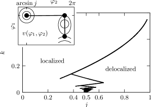
Figure 9: Phase diagram of the dynamically asymmetric dc- SQUID for weak damping and adiabatic ramping, $(\partial_{t}j\ll\tau_{1}^{-1}$). The critical line $j_{c}(k)$ is nearly identical with the one in the strong damping case, but is hysteretic along extensions of the critical lines $j_{c,n}^{+}(k)$. These are due to the nonzero kinetic energy acquired by the classical junction when sliding down in the new well formed after the tunneling of $\varphi_{2}$ at $j_{c,n}^{+}(k)$ and allowing $\varphi_{1}$ to surmount a residual potential barrier in the effective potential $\varepsilon_{0}(\varphi_{1})$. The inset illustrates the condition determining the termination point of the hysteretic line along $j_{c,1}^{+}(k)$. The three solid dots mark points of equal potential energies; the energy gained by the classical junction due to the phase slip of $\varphi_{2}$ just suffices to climb the top of the remaining barrier along $\varphi_{1}$.

A difference to the previous dissipative situation is given by the possibility to transform potential into kinetic energy. Ramping $j$ at fixed $k$ past the flux-entry line $j_{c,n}^{+}(k)$ triggers a phase slip in $\varphi_{2}$ and deforms the potential well in $\varepsilon_{0}(\varphi_{1})$ for the classical junction. The latter finds itself on the slope of the well and gains kinetic energy while sliding down towards the new minimum. The classical junction then may enter a running state if this kinetic energy gain is sufficient to surpass the barrier blocking the newly formed ($n$-th) minimum. Different from the overdamped case, the system then exhibits hysteretic behavior, as illustrated in the dynamical phase diagram Fig. 9, where the running state can be entered along extensions of the $j_{c,n}^{+}(k)$ line away from the phase boundary. The point where these extensions terminate is determined by the condition that the energy right after the tunneling of $\varphi_{2}$ is equal to the energy at the top of the barrier, as illustrated in the inset of Fig. 9. If the coupling $k$ is too small to lower the barrier sufficiently (cf. Fig. 7 (b)), the state of the heavy junction upon reaching $j=j_{c,n}^{+}(k)$ is transformed into a localized excited state of the newly formed potential well in $\varepsilon_{0}(\varphi_{1})$. Given the slow ramping $\partial_{t}j\ll\tau_{1}^{-1}$, the heavy junction relaxes to the ground state of the well and a further increase in $j$ is necessary to remove the barrier completely, hence the critical line jumps forward to $j_{c}(k)=j_{c,n}^{-}(k)$.

IV.2 Fast ramping of the bias current

We now turn to the case $\partial_{t}j\gg\omega_{p,1}$, where the ramping of $j$ is instantaneous with respect to the (massive) dynamics of the heavy junction; the final current $j$ has to remain below $\sim 0.7$, since fast ramping beyond this value allows the classical junction to overcome the potential barriers through conversion of potential to kinetic energy. Furthermore, we study the setting where $\omega_{p,1}\ll\tau_{2}^{-1},\tilde{\tau}_{2}^{-1}$; the quantum junction then has relaxed to the ground state (at $\varphi_{2}^{\mathrm{min},n}$) in the effective potential $v_{\mathrm{eff}}(\varphi_{2})$ before any motion of the heavy junction sets in. Hence, initially, the effective potential for the classical junction is given by the ground state energy $\varepsilon_{0}(\varphi_{1})$. The absence of Landau-Zener tunneling (due to the inequality (23)) then assures that the effective potential is given by $\varepsilon_{0}(\varphi_{1})$ during the entire motion of the classical junction.

We then can find the criterion for $\varphi_{1}$ to enter a running state: During the fast ramping of the current $j$, the heavy junction remains frozen at $\varphi_{1}=0$. We have to check whether the potential energy of the heavy junction is sufficient to overcome all barriers in $\varepsilon_{0}(\varphi_{1}>0)$; i.e., we have to inspect if the maximum of $\varepsilon_{0}(\varphi_{1})$ in the interval $0<\varphi_{1}<2\pi$ is realized at $\varphi_{1}=0$. As soon as this condition applies, the classical junction becomes delocalized. This analysis has to be performed numerically, and the result is displayed in Fig. 10. As a first overall result, we note that the critical current is shifted to lower values due to the instantaneous change of the effective potential for $\varphi_{1}$ by the fast ramping of the current and by the quantum decay of $\varphi_{2}$, allowing the heavy junction to transform potential into kinetic energy.

Another prominent change is in the form of the transition line, specifically, the ‘cut’ of the first tip of $j_{c}(k)$: The first segment at large values of $k$, cf. Fig. 10, corresponds to the conventional case for a ⁺-type line; the criterion for delocalization involves the full conversion of potential to kinetic energy of the heavy junction and the subsequent tunneling of the quantum junction right at the turning point of the classical junction, cf. inset (1) of Fig. 10. Following the $j_{c}^{+}(k)$-line further with decreasing $j$, we reach a point where the potential energy of the classical junction after the phase slip event is no longer sufficient to overcome the next barrier and an additional increase in $j$ is required to provide the missing energy. The segment (2) then involves partial conversion of the initial potential energy within the two wells before and after the phase slip event. Finally, moving along the segment (2) towards lower $k$ the value of $\varphi_{1}$ where the phase slip occurs decreases and finally reaches $\varphi_{1}=0$ (cf. Fig. 10, inset (3)). The critical line then continues along the third segment which is of the typical ^--type, with the quantum junction undergoing tunneling before the classical junction starts moving. After tunneling, a large current is required to lower the barrier in the cosine potential of the classical junction, cf. Fig. 10, inset (3). Note that the differentiation between positively sloped segments of type (1) and type (2) persists to segments determined by a higher fluxon index $n$, although the difference is invisible on the scale of Fig. 10.

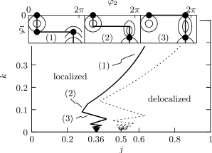
Figure 10: Effective critical current $j_{c}(k)$ (solid) of the current-biased dc-SQUID with strongly asymmetric parameters as a function of bias current $j$ and inverse inductance $k\propto 1/L$. We assume instantaneous ramping of the bias $j$ and a strictly classical and adiabatically slow (as compared to the dynamics of the quantum junction) motion of the weakly damped heavy degree of freedom $\varphi_{1}$. For comparison, the critical line of the dissipative case is also displayed (dashed line). The inset illustrates the three segments constituting the first part of $j_{c}(k)$, where solid dots indicate points of equal potential energy. Inset (3) shows the situation right at the tip between segments (2) and (3).

IV.3 Moderate ratios of $C_{1}/C_{2}$: Probabilistic effects

Above, we have assumed the limit of a very large ratio $C_{1}/C_{2}$. In the experiment, the dynamical asymmetry of the SQUID is implemented by shunting one of the two junctions with an external capacitance.Steffen:2006 This technique allows to reach large capacitance ratios of the order of $C_{1}/C_{2}\lesssim 10^{4}$. Given this finite mass ratio, one may enter a new dynamical regime where the classical junction is pulled out of its metastable state more efficiently. This is realized when the quantum junction attains a high energy state residing at the opposite side of the parabolic potential (large values of $\varphi_{2}$ in Fig. 8) and holds on to it while dragging the heavy junction out of its metastable state. This requires a fastfootnote4 current ramping $\partial_{t}j\gg 1/\tilde{\tau}_{2}$ (on the scale of the intervalley motion of the light junction), pushing the quantum junction to high potential energies during the ramp-up process. Furthermore, the condition $\omega_{p,1}\gg 1/\tilde{\tau}_{2}$ has to be satisfied to allow for motion of the heavy junction before relaxation of the quantum junction (from a side-well local ground state) back to the global minimum.

In order to simplify the situation, we assume a (weak) finite damping of the classical junction, $\omega_{p,1}^{-1}\ll\tau_{1}<\tilde{\tau}_{2}$, assuring that the classical junction relaxes before tunneling of the quantum junction (this assumption is merely a convenience, allowing us to ignore the availability of kinetic energy for the classical junction upon fast ramping). We then start from the local ground state of the original potential well at $\varphi_{1}=\varphi_{2}=\arcsin j$. The decay proceeds in the direction of $\varphi_{2}$ in the effective potential $v_{\mathrm{eff}}[\arcsin j](\varphi_{2})$ and can end up in any of the lower local ground states for the quantum junction. We denote the energy of the local ground state of the quantum junction in the $n$-th well by $\tilde{\varepsilon}_{0}^{n}$ (not to be confused with $\varepsilon_{n}$, the $n$-th excited state in the spectrum of the quantum junction). We estimate these energies as

$$\tilde{\varepsilon}_{0}^{n}(\varphi_{1})\approx v(\varphi_{1},\varphi_{2}^{\mathrm{min},n}),$$ (26)

where $\varphi_{2}^{\mathrm{min},n}(\varphi_{1})$ is the solution to Eq. (8) near $\varphi_{2}\approx 2\pi n$ at fixed $\varphi_{1}$ and we have neglected the zero point energy $\hbar\omega_{p,2}/2$.

The dynamics of $\varphi_{1}$ depends strongly on the fluxon index $n$ of the state of the quantum junction after the decay: the larger $n$, the stronger is the force on $\varphi_{1}$ facilitating its escape. We can define two extreme values for the critical current, a lower limit $j_{c}^{\scriptscriptstyle(1)}(k)$ arising from the largest attainable fluxon index $n$, and an upper limit $j_{c}^{\scriptscriptstyle(2)}(k)$ associated with the index $n$ of the global minimum of the quantum junction. We estimate the maximal index $n$ by comparing the energy of the state of the quantum junction before its inital decay with the height of the barrier blocking the access to the $n$-th minimum; the numerical solution of the relation

$$v_{\mathrm{eff}}[\varphi_{1}=\arcsin j](\varphi_{2}=\arcsin j)=v_{\mathrm{eff}}(\varphi_{2}^{\mathrm{max},n}),$$ (27)

with $\varphi_{2}^{\mathrm{max},n}$ the solution to Eq. (8) near $\varphi_{2}^{\mathrm{max}}\approx(2n-1)\pi$ at $\varphi_{1}=\arcsin j$ provides us with the line $j_{c,n}^{{\scriptscriptstyle(1)}+}(k)$. The subsequent stability analysis of $\varphi_{1}$ generates the lines $j_{c,n}^{{\scriptscriptstyle(1)}-}(k)$; their combination into $j_{c}^{\scriptscriptstyle(1)}(k)$ is displayed in Fig. 11.

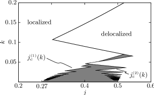
Figure 11: Effective critical currents of the dynamically asymmetric SQUID for $\tilde{\tau}_{2}\gg\omega_{p1}^{-1}$ and fast ramping. The system always turns resistive for $j>j_{c}^{\scriptscriptstyle(2)}(k)$ but never turns resistive for $j<j_{c}^{\scriptscriptstyle(1)}(k)$. For $j_{c}^{\scriptscriptstyle(1)}<j<j_{c}^{\scriptscriptstyle(2)}$ the delocalization of the system is determined by the statistical nature of the decay process of the quantum junction involving the side minima.

The shape of $j_{c}^{\scriptscriptstyle(2)}(k)$ is found as described before: We determine the index $n$ of the global minimum of $v_{\mathrm{eff}}(\varphi_{2})$ and deduce the motion of $\varphi_{1}$ in the effective potential $\tilde{\varepsilon}_{0}^{n}(\varphi_{1})$. The reduction in critical current due to the massive dynamics of $\varphi_{1}$ is not as pronounced as in Fig. 10, since the maximal critical current $j_{c}^{\scriptscriptstyle(2)}(k)$ involves the process where the classical junction dissipates most of its kinetic energy: the quantum junction decays to the $(n-1)$ fluxon state, the classical junction relaxes to its local minimum near $\varphi_{1}\gtrsim\arcsin j$, whereupon the quantum junction decays further to its global ground state with fluxon index $n$. Only the potential energy gained by the classical junction in the last step can be transformed to kinetic energy, making the resulting line shown in Fig. 11 differ from $j_{c}(k)$ in the overdamped case (Fig. 5).

The two critical lines $j_{c}^{\scriptscriptstyle(1)}(k)$ and $j_{c}^{\scriptscriptstyle(2)}(k)$ define a broad intermediate regime, see the grey area in Fig. 11, where the decay of the system is of probabilistic nature: whereas no Münchhausen decay is possible for $j<j_{c}^{\scriptscriptstyle(1)}(k)$, the decay of the system in the intermediate regime depends on which minimum the quantum junction $\varphi_{2}$ decays to. For $j>j_{c}^{\scriptscriptstyle(2)}(k)$ the system is always bound to decay.

The critical line $j_{c}^{\scriptscriptstyle(2)}(k)$ crosses twice the critical line $j_{c}^{\scriptscriptstyle(1)}(k)$ near $k\approx 0.5$ and for $n=2$. This special situation arises when the most distant accessible minimum and the global minimum are neighbors (with indices $n=2$ and $n=1$) and hence strongly interrelated. With decreasing $k$, both the height of the maximum near $\varphi_{2}\approx 3\pi$ (determining $j_{c}^{\scriptscriptstyle(1)}(k)$) and the position of the minimum at $\varphi_{2}\approx 4\pi$ ($n=2$) with respect to the one at $\varphi_{2}\approx 2\pi$ ($n=1$; the competition between these minima defines $j_{c}^{\scriptscriptstyle(2)}(k)$) are lowered. The latter effect is slightly stronger, leading to the crossing of the lines under a small angle. Upon further lowering of $k$, the relevant fluxon index for $j_{c}^{\scriptscriptstyle(1)}(k)$ increases twice as fast as for $j_{c}^{\scriptscriptstyle(2)}(k)$, preventing any further crossings of the critcal lines.

To guarantee reasonable time scales in the experiment requires a fast quantum dynamics near the global minimum, hence the ratio $E_{J}/\hbar\omega_{p,2}$ should be small, of order unity. For a fast ramping, this is in conflict with the requirement of large $\tilde{\tau}_{2}$ in all side-wells; as a result, not all reachable side minima may be relevant for the dynamics of $\varphi_{1}$ (i.e., $\tilde{\tau}_{2}\gg\omega_{p,1}^{-1}$ does not hold), effectively shifting the lower critical current $j_{c}^{\scriptscriptstyle(1)}(k)$ to larger values.

So far we have neglected any quantum corrections for the variable $\varphi_{1}$; however, with a finite ratio $C_{1}/C_{2}$ such corrections may become relevant. Modifications due to quantum fluctuations in the heavy degree of freedom are twofold: On the one hand, we have disregarded the tunneling of $\varphi_{1}$ through a small residual barrier, leading to a broadening of all lines of the ^--type. On the other hand, we have assumed the dynamics of $\varphi_{2}$ to occur in the effective potential $v_{\mathrm{eff}}[\varphi_{1}](\varphi_{2})$, with $\varphi_{1}$ fixed, while for a finite value of $C_{1}$ the ground state wave function of the heavy junction acquires a finite width of the order of $\delta\varphi_{1}\sim(8E_{c1}/E_{J})^{1/4}$. This leads to a broadening of all lines of the ⁺-type, which can be interpreted as $\varphi_{1}$ taking part in the tunneling of $\varphi_{2}$.

V Experimental Implementation

The running state following a Münchhausen decay is associated with a finite time-averaged voltage across the device. The above results thus can be tested experimentally by measuring the voltage drop as a function of the applied bias current $J$ and of the inductance $L$ of the SQUID.

Mapping any part of $j_{c}(k)$ requires changing the coupling $k\propto L^{-1}$. The latter is determined by the total inductance of the loop $L=L_{\mathrm{geo}}+L_{\mathrm{kin}}$, comprising the geometric ($L_{\mathrm{geo}}$) and kinetic ($L_{\mathrm{kin}}$) inductances of the loop. The former is of the order of the loop perimeter and accounts for the magnetic field energy. The kinetic inductance relates to the geometric quantity via $L_{\mathrm{kin}}\sim L_{\mathrm{geo}}\lambda^{2}/r^{2}$, with $r$ the radius of the wire and $\lambda$ denoting the superconducting penetration depth. Usually, the inductance is dominated by its geometric part. However, a large inductance, as desired for our setup, can be installed by using a thin wire. Furthermore, the inductance is fixed after fabrication and its modification (e.g., via installing a diamagnetic shield) is rather difficult. Another way to trace the critical current line is obtained by applying an external magnetic flux $\Phi_{e}$ to the sample, in which case the potential Eq. (2) has to be replaced by

$$v(\varphi_{1},\varphi_{2})=1-\cos\varphi_{1}+1-\cos\varphi_{2}\\ -j(\varphi_{1}+\varphi_{2})+\frac{k}{2}(\varphi_{1}-\varphi_{2}-2\pi\Phi_{e}/\Phi_{0})^{2}.$$ (28)

The critical current $j_{c}$ then can be studied as a function of $\Phi_{e}$. The analysis proceeds in the same way as before: a change in $k$ altering the opening angle of the parabola in $v(\varphi_{1},\varphi_{2})$ is replaced by a shift in the parabola’s position due to the applied flux $\Phi_{e}$.

Figure 12: Phase diagram of the dynamically asymmetric SQUID in the strong damping case as a function of the externally applied flux $\Phi_{e}$ and bias current $j$. Here, the coupling $k\propto L^{-1}$ is fixed at a value $k=0.06$; the critical lines in the diagram correspond to $n=2$. The critical line is periodic in $\Phi_{e}$ with a period $\Phi_{0}$, a consequence of the invariance under the replacements $\Phi_{e}/\Phi_{0}\rightarrow\Phi_{e}/\Phi_{0}\pm 1$ and $n\rightarrow(n\pm 1)$.

As an illustration, we discuss here the most simple case of an overdamped dynamics, analogous to Sec. III. In a first step, the system relaxes to the ground state at the minimum of the potential $v(\varphi_{1},\varphi_{2})$, Eq. (28), as given by the solutions $\varphi_{1}^{\mathrm{min}},\varphi_{2}^{\mathrm{min}}$ of

$$\sin(\varphi_{1}^{\mathrm{min}})-j+k\left(\varphi_{1}^{\mathrm{min}}-\varphi_{2}^{\mathrm{min}}-2\pi\frac{\Phi_{e}}{\Phi_{0}}\right)\! = \!0,$$ (29)

$$\sin(\varphi_{2}^{\mathrm{min}})-j-k\left(\varphi_{1}^{\mathrm{min}}-\varphi_{2}^{\mathrm{min}}-2\pi\frac{\Phi_{e}}{\Phi_{0}}\right)\! = \!0,$$ (30)

near $\varphi_{1}^{\mathrm{min}}\approx\varphi_{2}^{\mathrm{min}}\approx 0$. The critical line $j^{+}_{c,n}(\Phi_{e})$ then derives from the condition

$$k\approx\frac{j}{(2n-1)\pi-\varphi_{1}^{\mathrm{min}}(\Phi_{e})+2\pi\Phi_{e}/\Phi_{0}},$$ (31)

where both the shift of the parabola $v_{\mathrm{eff}}(\varphi_{2})$ by $2\pi\Phi_{e}/\Phi_{0}$ and the flux dependence of $\varphi_{1}^{\mathrm{min}}$ are accounted for. Similarly, Eq. (14) for $k_{c,n}^{-}(j)$ is changed to

$$k\approx\frac{1-j}{(2n-1/2)\pi+\arcsin(2j-1)+2\pi\Phi_{e}/\Phi_{0}},$$ (32)

from which we find the critical lines $j^{-}_{c,n}(\Phi_{e})$. The results of Eqs. (29) - (32) are invariant under the shifts $\Phi_{e}/\Phi_{0}\rightarrow\Phi_{e}/\Phi_{0}\pm 1$ and $n\rightarrow(n\pm 1)$. The Münchhausen decay thus can be studied within a finite interval, e.g. $\Phi_{e}/\Phi_{0}\in[-0.5,0.5]$, and the resulting phase diagram is displayed in Fig. 12.

Biasing the SQUID with an external magnetic flux has a convenient side effect: For negative flux $\Phi_{e}$, the crossing point of $j_{c,n}^{+}(k)$ and $j_{c,n}^{-}(k)$ is shifted to larger values of $k$ and the tunneling barrier for $\varphi_{2}$ is lowered, allowing to study the Münchhausen effect using a SQUID with considerably smaller inductance and hence smaller size.

VI Conclusion

We have shown how a system consisting of a ‘quantum’ degree of freedom coupled to a ‘classical’ one, implemented with a two-junction SQUID, can perform a complex decay process out of a zero-voltage state involving quantum tunneling of the ‘light’ junction and classical motion of the ‘heavy’ junction. We have analyzed the cases of strong and weak damping, for different methods of preparation (fast and slow ramping), and for various ratios of the capacitances $C_{1}/C_{2}$ and have found the effective critical current $j_{c}(k)$ exhibiting a common characteristic shape. Its zig-zag like structure originates in two competing effects: while the number $n$ of flux units which can enter the SQUID is increased with decreasing $k$, the current redirected over the heavy junction at given $n$ is decreased. For junctions with equal critical currents, the critical line approaches the value $j_{c}(k\rightarrow 0)\rightarrow 1/2$ in the dissipative case; asymmetries in the critical currents of the two junctions lead to a shift of the critical line $j_{c}(k)$ to values straddling the critical current of the heavy junction. Going over from dissipative to massive dynamics, the kinetic energy stored in the system allows to better overcome the potential barriers and the critical line shifts to smaller values of $j$; furthermore, hysteretic effects, similar to the situation encountered for underdamped junctions, and even probabilistic behavior may show up.

- (1) B.D. Josephson, Phys. Lett. 1, 251 (1962).
- (2) We use modified Gaussian units, where and are measured in units of length.
- (3) R.F. Voss and R.A. Webb, Phys. Rev. Lett. 47, 265 (1981).
- (4) A.O. Caldeira and A.J. Leggett, Phys. Rev. Lett. 46, 211 (1981).
- (5) A.O. Caldeira and A.J. Leggett, Ann. Phys. (NY) 149, 374 (1983).
- (6) M.H. Devoret, J.M. Martinis, and J. Clarke, Phys. Rev. Lett. 55, 1908 (1985).
- (7) J.M. Martinis, M.H. Devoret, and J. Clarke, Phys. Rev. Lett. 55, 1543 (1985).
- (8) J.M. Martinis, M.H. Devoret, and J. Clarke, Phys. Rev. B 35, 4682 (1987).
- (9) S. Chakravarty and A.J. Leggett, Phys. Rev. Lett. 52, 5 (1984).
- (10) A.J. Leggett, S. Chakravarty, A.T. Dorsey, M.P.A. Fisher, A. Garg, and W. Zwerger, Rev. Mod. Phys. 59, 1 (1987).
- (11) Y. Nakamura, C.D. Chen, and J.S. Tsai, Phys. Rev. Lett. 79, 2328 (1997).
- (12) Y. Nakamura, Y.A. Pashkin, and J.S. Tsai, Nature 398, 786 (1999).
- (13) J.R. Friedman, V. Patel, W. Chen, S.K. Tolpygo, and J.E. Lukens, Nature 406, 43 (2000).
- (14) C.H. van der Wal, A.C.J. ter Haar, F.K. Wilhelm, R.N. Schouten, C.J.P.M. Harmans, T.P. Orlando, S. Lloyd, and J.E. Mooij, Science 290, 773 (2000).
- (15) I. Chiorescu, Y. Nakamura, C.J.P.M. Harmans, and J.E. Mooij, Science 299, 1869 (2003).
- (16) S.-X. Li, Y. Yu, Y. Zhang, W. Qiu, S. Han, and Z. Wang, Phys. Rev. Lett. 89, 098301 (2002).
- (17) F. Balestro, J. Claudon, J.P. Pekola, and O. Buisson, Phys. Rev. Lett. 91, 158301 (2003).
- (18) Y.-C. Chen, J. Low Temp. Phys. 65, 133 (1986).
- (19) B.I. Ivlev and Y.N. Ovchinnikov, Sov. Phys. JETP 66, 378 (1987).
- (20) C. Morais Smith, B. Ivlev, and G. Blatter, Phys. Rev. B 49, 4033 (1994).
- (21) A similar setup with one tunable small (s) and one large (l) Josephson junction was used previously as a qubit (s) with integrated readout (l).Chiarello:2005 ; Castellano:2005 ; Chiarello:2007
- (22) F. Chiarello, P. Carelli, M.G. Castellano, C. Cosmelli, L. Gangemi, R. Leoni, S. Poletto, D. Simeone, and G. Torrioli, Supercond. Sci. Tech. 18, 1370 (2005).
- (23) M.G. Castellano, F. Chiarello, R. Leoni, G. Torrioli, P. Carelli, C. Cosmelli, M. Di Bucchianico, and D. Simeone, IEEE Trans. Appl. Supercond. 15, 849 (2005).
- (24) F. Chiarello et al., IEEE Trans. Appl. Supercond. 17, 124 (2007).
- (25) A.U. Thomann, V.B. Geshkenbein, and G. Blatter, Physica C 468, 705 (2008).
- (26) O. Hallatschek, Diploma Thesis, 2000.
- (27) W.-T. Tsang and T.V. Duzer, J. Appl. Phys. 46, 4573 (1975).
- (28) V. Lefevre-Seguin, E. Turlot, C. Urbina, D. Esteve, and M.H. Devoret, Phys. Rev. B 46, 5507 (1992).
- (29) S.E. Korshunov, Sov. Phys. JETP 65, 1025 (1987).
- (30) D. Esteve, M.H. Devoret, and J.M. Martinis, Phys. Rev. B 34, 158 (1986).
- (31) D.V. Averin, J.R. Friedman, and J.E. Lukens, Phys. Rev. B 62, 11802 (2000).
- (32) While the correction might not be immaterial, its dependence on is small.
- (33) M. Steffen, M. Ansmann, R. McDermott, N. Katz, R.C. Bialczak, E. Lucero, M. Neeley, E.M. Weig, A.N. Cleland, and J.M. Martinis, Phys. Rev. Lett. 97, 050502 (2006).
- (34) When the ramping is slow, the modifications with respect to the discussion in Sec. IV.1 are negligible: Due to the slow ramping, the quantum junction remains always in its ground state and hence the classical junction moves adiabatically in the effective potential created by the quantum junction. The resulting critical current is identical to the one presented in Fig. 9.