Self-organization in dissipative optical lattices

Abstract

We show that the transition from Gaussian to the $q$-Gaussian distributions occurring in atomic transport in dissipative optical lattices can be interpreted as self-organization by recourse to a modified version of Klimontovich’s S-theorem. As a result, we find that self-organization is possible in the transition regime, only where the second moment $\left\langle p^{2}\right\rangle$ is finite. Therefore, the nonadditivity parameter $q$ is confined within the range $1<q<\frac{5}{3}$, although whole spectrum of $q$ values i.e., $1<q<3$, is considered theoretically possible. The range of $q$ values obtained from the modified S-theorem is also confirmed by the experiments carried out by Douglas et al. [Phys. Rev. Lett. 96, 110601 (2006)].

I
Introduction

The importance of understanding physical phenomena exhibiting asymptotical inverse power law distributions becomes apparent if we consider its emergence in such diverse fields as subregion laser cooling [1], the heartbeat histograms of healthy patients [2], blinking nanocrystals [3], rheology of steady-state draining foams [4], econophysics [5], earthquake models [6], to name but a few.

One such distribution is the Tsallis distribution [7], which found many applications in different fields [8]. Recently, it was pointed out that the momentum distribution of cold atoms in a dissipative optical lattice is a Tsallis distribution [9]. Soon, this theoretical prediction has been verified experimentally [10].

Three different regimes of atomic transport is possible in an optical lattice (see Ref. [11] for details), depending on the depth of the optical potential. In the intermediate regime between the diffusive motion in deep potentials and ballistic motion in shallow potentials, the atomic transport is governed by the Tsallis distribution [9, 10]. In fact, it has been shown, both theoretically and experimentally, that a transition from an ordinary Gaussian to the $q$-Gaussian distribution occurs by changing the ratio of the recoil energy to the potential depth [9, 10].

Our aim in this paper is to show that this transition can be interpreted as a self-organization in the context of modified S-theorem. Klimontovich [12-17] originally proposed S-theorem (Self-organization theorem) in order to generalize Gibbs’ theorem [18] to open systems, since the latter rests on the assumption that all the compared distributions have the same mean energy values. However, this assumption does not hold when one studies open systems where the mean energy of the system is not constant due to the interaction of the system with the environment (e.g., a laser field in the case of optical lattices). Therefore, Klimontovich defined a quantity called effective energy. Equating the mean effective energies of different states and then comparing the associated entropies, he showed that S-theorem orders the associated entropies in such a way that the state closer to equilibrium possesses a greater entropy compared to the other states. In other words, we have a more ordered state as the control parameter increases. This decrease of entropy on ordering is called self-organization by Haken [19]. We also mention that the process of equating mean effective energies of different states is called renormalization by Klimontovich. As a result, S-theorem did not only succeed in generalizing Gibbs’ theorem but gained recognition as a criterion of self-organization in open systems, since it allows us to compare even the stationary nonequilibrium distributions [12-17].

We also mention that the use of S-theorem is not limited to analytical models. It has also been used for many numerical models such as logistic map [20], heart rate variability [21, 22] and the analysis of electroencephalograms of epilepsy patients [23] as a criterion of self-organization.

However, S-theorem rests on the use of Boltzmann-Gibbs (BG) entropy. Therefore, it is useful to analyze transition regimes where the stationary distributions are of exponential form. On the other hand, the study of open systems may result in stationary distributions of the inverse power law form. Motivated by this fact, a generalization of the S-theorem has recently been provided by the employment of nonadditive Tsallis entropy [24, 25]. This generalized nonadditive S-theorem can be used to analyze the transition regimes in open systems, where the stationary distributions are $q$-exponentials, which asymptotically yield to inverse power law distributions.

Although the dissipative optical lattices serve as open systems due to their interaction with laser fields, neither original S-theorem due to Klimontovich nor its nonadditive generalization can be used for the description of self-organization in the aforementioned intermediate region of atomic transport. The reason is that this region exhibits a transition from Gaussian to $q$-Gaussian distributions. Therefore, the intermediate region requires an intermediate treatment between the two formulations of the S-theorem. This intermediate S-theorem, called modified S-theorem, is provided here for the explicit purpose of applying it to the dissipative optical lattices.

The paper is organized as follows: In Section II, we review the original (i.e., additive) and nonadditive S-theorems for open systems. The modified S-theorem and its immediate application to dissipative open lattices are presented in Section III. Concluding remarks will be presented in Section IV.

II The additive and nonadditive S-theorems

The additive S-theorem due to Klimontovich [12-17] requires the use of two distinct probability distributions, i.e., $r_{eq}$ and $p$, corresponding to equilibrium and nonequilibrium states, respectively. The stationary equilibrium distribution is defined as the distribution corresponding to the state where the relevant control parameter is set to zero. Similarly, any other stationary state with non-zero control parameter is defined as the nonequilibrium state. As the value of the control parameter increases, the system recedes away from equilibrium state. By Gibbs’ theorem, we know that mere substitution of these distributions into BG entropy will yield nonsensical results due to the failure of the equal mean energy assumption because of the interaction with the environment. Therefore, Klimontovich [12-17] renormalizes the equilibium distribution i.e., $r_{eq}$. However, we note that the S-theorem of Klimontovich is not limited to the comparisons of equilibrium and nonequilibrium distributions. It can be used to compare any two stationary distributions as long as they are different from one another through the change in the value of the control parameter. From now on, we will drop the subscript $(eq)$ from the equilibrium probability distribution $r$. Therefore, it should be understood that the probability distribution $r$ denotes the equilibrium distribution. Next, Klimontovich defines a quantity called effective energy $U_{\text{eff}}$ [12-17] in terms of the equilibrium state as

$$U_{\text{eff}}=-\ln r.$$ (1)

The definition of effective energy in Eq. (1) is central to the S-theorem, and therefore requires some explanation. The application of the effective energy definition in Eq. (1) to the equilibrium distribution results in $U_{\text{eff}}=\beta\varepsilon_{i}$ (apart from normalization). This explains why it is called effective energy since it is proportional to the multiplication of the Lagrange multiplier $\beta$ associated with the internal energy constraint and the energy of the $i$th microstate. Consequently, its average corresponds to the $\beta$ times the average internal energy of the equilibrium distribution. We then equate the effective energy of the equilibrium and nonequilibrium states and this equalization procedure is called renormalization by Klimontovich. As a result of this renormalization, we no longer use the equilibrium distribution $r$, but the renormalized equilibrium distribution $\widetilde{r}$, where tilde denotes that the renormalization is taken care of. Explicitly written, the renormalization reads

$$\left\langle U_{\text{eff}}\right\rangle^{(req)}=\left\langle U_{\text{eff}}\right\rangle^{(neq)},$$ (2)

where superscripts $(req)$ and $(neq)$ denote the renormalized equilibrium and ordinary nonequilibrium states, respectively. Then, S-theorem is equivalent to showing that the renormalized entropy $R[p\|{\widetilde{r}}]$ defined as

$$R[p\|{\widetilde{r}}]\equiv\ S_{BG}^{neq}(p)-\widetilde{S}_{BG}^{eq}(\widetilde{r})$$ (3)

is negative i.e., $R[p\|{\widetilde{r}}]<0$, since this implies that $\widetilde{S}_{BG}^{eq}>S_{BG}^{neq}$, where $S_{BG}$ is the usual BG entropy given by

$$S_{BG}(p)=-\sum_{i=1}^{W}p_{i}\ln p_{i},$$ (4)

where $p_{\text{i }}$ is the probability of the system in the $i$th microstate, $W$ is the total number of the configurations of the system.

The proof of the S-theorem relies on the definition of Kullback-Leibler relative entropy (KL) [26], which reads

$$K[p\|{r}]=\sum_{i=1}^{W}p_{i}\ln\left(\frac{p_{i}}{r_{i}}\right),$$ (5)

since the renormalized entropy given in Eq. (3) is, through the renormalization in Eq. (1), equal to

$$R[p\|{\widetilde{r}}]=-K[p\|{\widetilde{r}}].$$ (6)

The S-theorem is therefore proven [27], since KL entropy is positive definite i.e.,

$$R[p\|{\widetilde{r}}]<0.$$ (7)

Although Klimontovich’s S-theorem is a generalization of the Gibbs’ theorem, it is based on the use of exponential stationary distributions and therefore BG entropy. Therefore, the S-theorem due to Klimontovich cannot be used in the case of inverse power law stationary distributions. In order to overcome this difficulty, a new generalization of S-theorem has been given in the framework of nonadditive thermostatistics. This nonadditive S-theorem first generalizes the effective energy by deforming the logarithm in Eq. (1) as

$$U_{\text{eff}}=\ln_{q}\left(\frac{1}{r_{eq}}\right),$$ (8)

where the $q$-logarithm function $\ln_{q}(x)$ is defined as

$$\ln_{q}(x)=\frac{x^{1-q}-1}{1-q}.$$ (9)

The nonadditive S-theorem can be similarly written as

$$R_{q}[p\|\widetilde{r}]=S_{q}(p)-\widetilde{S}_{q}(\widetilde{r})=-K_{q}[p\|\widetilde{r}]<0,$$ (10)

for positive values of the nonadditivity parameter $q$, where the nonadditive Tsallis entropy $S_{q}$ [24, 25] is given by

$$S_{q}(p)=\frac{\sum_{i}^{W}p_{i}^{q}-1}{1-q}$$ (11)

and the nonadditive relative entropy $K_{q}[p\|\widetilde{r}]$ [28] is given by

$$K_{q}[p\|\widetilde{r}]=\frac{\sum_{i}p_{i}^{q}}{q-1}+\sum_{i}\widetilde{r}_{i}^{q}-\frac{q}{q-1}\sum_{i}p_{i}\widetilde{r}_{i}^{q-1}.$$ (12)

The proof of the nonadditive S-theorem is limited to the positive $q$ values only, since the nonadditive relative entropy is positive only in this region. However, we can exclude negative $q$ values, since Tsallis entropy is stable only for positive values of $q$ [29].

It should be noted that the ordinary S-theorem by Klimontovich is recovered in the $q\rightarrow 1$ limit. This can be seen from the inspection of Eq. (10), since Tsallis entropy expressions become BG entropies, whereas all the stationary distributions become exponential in the $q\rightarrow 1$ limit. The nonadditive relative entropy in Eq. (12) becomes KL relative entropy in the aforementioned limit i.e., $K[p\|r]\equiv\sum_{i}p_{i}\ln(p_{i}/r_{i})$ [26, 28], which is positive definite, ensuring the negativity of the ordinary renormalized entropy.

III optical lattices and Modified S-theorem

In the previous section, we reviewed two interrelated criteria of self-organization, namely, the additive and nonadditive S-theorems. The former can be used when there are exponential stationary distributions so that one can use BG entropy together with the renormalization of effective energies of stationary states. The latter, on the other hand, is used when the stationary distributions are $q$-exponentials associated with the Tsallis entropy. However, self-organization is not limited to the transitions amongst exponential or $q$-exponential stationary distributions. An intermediate transition is possible so that a transition from an exponential to $q$-exponential stationary distribution may be observed. In this case, neither additive nor nonadditive S-theorems can be used.

Such a transition has recently been observed in anomalous transport experiments in optical lattices [10]. Before proceeding further, it is important to review how the transition from an ordinary exponential stationary distribution to the $q$-exponential distribution can occur [9]. In order to do so, one first needs to derive the master equation, which describes the atom-laser interaction in the optical lattice. Assuming that the laser intensity is low and the atoms move fast, a semiclassical treatment is possible, which allows one to obtain, after spatial averaging, so-called Rayleigh equation for the semiclassical Wigner function $W(p,t)$

$$\frac{\partial W}{\partial t}=-\frac{\partial}{\partial p}\left[K(p)W\right]+\frac{\partial}{\partial p}\left[D(p)\frac{\partial W}{\partial p}\right],$$ (13)

where the variables $p$ and $t$ denote momentum and time, respectively [30, 31, 32]. The drift coefficient $K(p)$ and diffusion factor $D(p)$ satisfy the relation [33]

$$\frac{K\left(p\right)}{D\left(p\right)}=-\frac{\beta}{1-\beta\left(1-q\right)U\left(p\right)}\frac{\partial U\left(p\right)}{\partial p},$$ (14)

where

$$q=1+a_{c}\;\;\;\;\;;\;\;\;\;\;U\left(p\right)=p^{2}.$$ (15)

The parameter $\beta$ is positive and can be expressed in terms of the microscopic damping and diffusion coefficients [9]. The term $a_{c}$ denotes the control parameter, which represents the interaction of the atom with the environment i.e., laser field. The control parameter can be written more explicitly in terms of the microscopic parameters [9] as

$$a_{c}=\frac{2D_{0}}{\alpha p_{c}^{2}}.$$ (16)

The terms $\alpha$ and $p_{c}$ denote the damping coefficient and the capture momentum, respectively. The term $D_{0}$ is the diffusion term associated with the fluctuations due to spontaneous photon emissions and fluctuations in the difference of photons absorbed in the two laser beams [9]. Note that the control parameter $a_{c}$ can also be written in terms of the potential depth $U_{0}$ and the recoil energy $E_{R}$ [30] as

$$a_{c}=\frac{44E_{R}}{U_{0}}.$$ (17)

Since the condition (14) is satisfied in optical lattices, the exact stationary solution to the Rayleigh equation in Eq. (13) is given in terms of the $q$-Gaussians

$$W_{q}\left(p\right)=C_{q}\left[1-\beta\left(1-q\right)U\left(p\right)\right]^{1/\left(1-q\right)},$$ (18)

where we also require $W_{q}\left(p\right)\rightarrow 0$ when $p\rightarrow\pm\infty$ When the control parameter is equal to zero, the nonadditivity parameter $q$ becomes equal to 1. We then have stationary equilibrium distribution of the Gaussian form i.e.,

$$W_{1}\left(p\right)=C_{1}\exp\left[-\beta U\left(p\right)\right].$$ (19)

As the interaction between the atoms and the laser field is turned on, the control parameter $a_{c}$ takes nonzero positive values. As a result, the value of the nonadditivity parameter $q$ exceeds 1 so that we have stationary nonequilibrium distribution of $q$-Gaussian form given by Eq. (18).

As we remarked earlier, this transition from an ordinary exponential stationary distribution to a $q$-Gaussian distribution cannot be analyzed within the frameworks of the aforementioned versions of the S-theorem. Therefore, we need a modified S-theorem, which can be used as a criterion of self-organization for the transition from Gaussian to $q$-Gaussian regime.

Since the equilibrium distribution is an ordinary Gaussian, the modified S-theorem must include BG entropy associated with the Gaussian equilibrium distribution as is the case with the original, additive S-theorem by Klimontovich [12-17]. On the other hand, the stationary nonequilibrium distribution is a $q$-Gaussian. Therefore, the entropy of the stationary nonequilibrium distribution must be calculated by using Tsallis entropy as in the nonadditive S-theorem [24, 25]. The modified S-theorem will be the difference of these two entropies together with the renormalization condition.

The only ingredient left is how the renormalization will be carried out in the modified S-theorem. However, the renormalization condition can be borrowed from Klimontovich’s S-theorem [12-17] as it is, since the equilibrium distribution associated with the original and modified S-theorems both is of the same form i.e., exponential. Therefore, similar to Eq. (1), we can write

$$U_{\text{eff}}=-\ln W_{1}\left(p\right)$$ (20)

and then use Eq. (2) to obtain

$$\left\langle p^{2}\right\rangle^{(req)}=\left\langle p^{2}\right\rangle^{(neq)},$$ (21)

where we have inserted Eq. (20). The renormalized entropy $\Re[W_{q}\|\widetilde{W}_{1}]$ corresponding to the modified S-theorem can then be written as

$$\Re[W_{q}\|\widetilde{W}_{1}]=S_{q}(W_{q})-\widetilde{S}_{BG}(\widetilde{W}_{1}).$$ (22)

Similar to the additive and nonadditive versions of S-theorem, we calculate $\Re[W_{q}\|\widetilde{W}_{1}]$ and see whether it becomes negative for some interval of $q$ values. Before proceeding with the renormalization condition given by Eq. (21), we write the equilibrium

$$W_{1}\left(p\right)=\sqrt{\frac{4\beta}{\pi}}\exp\left[-\beta p^{2}\right]$$ (23)

and the stationary nonequilibrium distribution

$$W_{q}\left(p\right)=\sqrt{4\beta\left(q-1\right)}\left[B\left(\frac{1}{2},\frac{3-q}{2q-2}\right)\right]^{-1}\left[1-\beta\left(1-q\right)p^{2}\right]^{1/\left(1-q\right)}\;\;\;;\;\;\;1<q<3,$$ (24)

by inserting the normalization constants $C_{1}$ and $C_{q}$ explicitly. The term $B\left(x,y\right)$ denotes the Beta function [34]. We now rewrite Eq. (21)

$$\int\limits_{0}^{\infty}dpp^{2}\widetilde{W}_{1}\left(p\right)=\int\limits_{0}^{\infty}dpp^{2}W_{q}\left(p\right).$$ (25)

By substituting Eqs. (23) and (24) into Eq. (25), we obtain the renormalized inverse temperature $\widetilde{\beta}$ as

$$\widetilde{\beta}=\frac{\left(q-1\right)\Gamma\left(\frac{3-q}{2q-2}\right)}{\Gamma\left(\frac{5-3q}{2q-2}\right)}\beta\;\;\;;\;\;\;1<q<\frac{5}{3},$$ (26)

where $\Gamma\left(x,y\right)$ is the Gamma function [34]. The associated equilibrium

$$\widetilde{S}_{BG}\left(\widetilde{W}_{1}\right)=\frac{1}{2}-\frac{1}{2}\ln\left(\frac{4\widetilde{\beta}}{\pi}\right)\;\;\;;\;\;\;1<q<\frac{5}{3}$$ (27)

and nonequilibrium entropies can be calculated

$$S_{q}\left(W_{q}\right)=\frac{1-\left[4\beta\left(q-1\right)\right]^{\frac{q-1}{2}}\left[B\left(\frac{1}{2},\frac{3-q}{2q-2}\right)\right]^{-q}B\left(\frac{1}{2},\frac{q+1}{2q-2}\right)}{q-1}\;\;\;;\;\;\;1<q<\frac{5}{3},$$ (28)

where the renormalized inverse temperature $\widetilde{\beta}$ in Eq. (27) can be substituted from Eq. (26). Finally, the renormalized entropy reads

$$\Re[W_{q}\|\widetilde{W}_{1}]=\frac{1-\left[4\beta\left(q-1\right)\right]^{\frac{q-1}{2}}\left[B\left(\frac{1}{2},\frac{3-q}{2q-2}\right)\right]^{-q}B\left(\frac{1}{2},\frac{q+1}{2q-2}\right)}{q-1}-$$

$$\frac{1}{2}+\frac{1}{2}\ln\left[\frac{4\left(q-1\right)\Gamma\left(\frac{3-q}{2q-2}\right)}{\Gamma\left(\frac{5-3q}{2q-2}\right)\pi}\beta\right]\;\;\;;\;\;\;1<q<\frac{5}{3}.$$ (29)

The renormalized entropy $\Re[W_{q}\|\widetilde{W}_{1}]$ in Eq. (III) is indeed negative in the interval $1<q<\frac{5}{3}$ as can be seen from Fig. 1, independent of the value of $\beta$. It corresponds to an entropy decrease when the entropies of the states are evaluated with the consistent expressions of entropy i.e., the Gaussian distribution at equilibrium with BG entropy and $q$-Gaussian distributions at nonequilibrium with the Tsallis entropy. As the control parameter $a_{c}$ increases from zero (i.e., as the nonadditivity parameter $q$ increases from 1), the system moves from Gaussian distribution to $q$-Gaussian distributions, decreasing its entropy. This indicates that the transition from the Gaussian distribution to the $q$-Gaussian distributions in dissipative optical lattices is self-organization, signifying a transition to a more ordered state. It can be seen from Fig. 2b of Douglas et al. [10] that the self-organization interval determined by the modified S-theorem i.e., $1<q<\frac{5}{3}$, is confirmed by the experiment, although the whole range of admissible $q$ values is theoretically $1<q<3$.

We also remark that the renormalized inverse temperature $\widetilde{\beta}$ is a linear function of the ordinary inverse temperature $\beta$ as can be seen from Eq.(26). Therefore, the procedure of renormalization does not deform the equilibrium distribution, which is an exponential. Its role is to compensate the difference between the equilibrium temperature associated with the Gaussian distribution and the parameter $\beta$ in the $q$-Gaussian distribution, since the latter is not physical temperature. This compensation is equivalent to heating up the equilibrium temperature of the system as a result of the linear decrease of $\widetilde{\beta}$ with respect to $\beta$ for all $q$ values in the range $1<q<\frac{5}{3}$. The fact that $\widetilde{\beta}$ depends explicitly on $q$ implies that the renormalization also takes the microscopic structure into account.

We finally mention the effect of renormalization on the spatial correlation function $G\left(a\right)=\int dx\psi\left(x,t\right)\psi^{\ast}\left(x+a,t\right)$, where $\psi\left(x,t\right)$ denotes the wave function at time $t$ [35]. The spatial correlation function can be considered as a measure of how coherent a state is between two different points. For a Gaussian wave packet such as $W_{1}$, the spatial correlation function too is a Gaussian with a correlation length $\lambda=2\hslash\sqrt{\beta}$ [9]. The renormalized correlation length, on the other hand, is equal to $\widetilde{\lambda}=2\hslash\sqrt{\left(q-1\right)\Gamma\left(\frac{3-q}{2q-2}\right)/\Gamma\left(\frac{5-3q}{2q-2}\right)\beta}$ in the interval $1<q<\frac{5}{3}$. Therefore, we conclude that the correlation length decreases with increasing value of the nonadditivity parameter $q$. In other words, the Gaussian distribution becomes less coherent spatially as a result of the renormalization procedure employed in the modified S-theorem. This decrease in coherence becomes more dominant as the system moves further from equilibrium.

IV Conclusions

By analyzing the intermediate anomalous transport regime in dissipative optical lattices [9, 10] in the framework of a modified version of Klimontovich’s S-theorem, we have shown that the self-organization occurs in the transition from Gaussian to the $q$-Gaussian distributions, implying an entropy decrease i.e., a more ordered state as the system is driven out of equilibrium as a result of the interaction of the atoms with the laser field.

An interesting result of the modified S-theorem is that it confines the self-organization in the region $1<q<\frac{5}{3}$, although, for example, there is nothing which forbids transition to a region with $q=2$, (note that the $q$-Gaussian distributions are normalizable in the whole range $1<q<3$). This is also confirmed with the experimental results obtained by Douglas et al. [10]. The reason for this confinement is due to the additional requirement associated with the (modified) S-theorem i.e., renormalization of the effective energy. For dissipative optical lattices, the effective energy term corresponds to the square of the momentum. Therefore, the procedure of renormalization confines the self-organization to the region, where the second moment of the distribution $\left\langle p^{2}\right\rangle$ converges. This is similar to the requirement of finite capture momentum for the occurrence of $q$-Gaussian distribution in dissipative optical lattices [9]. If the capture momentum $p_{c}$ is infinite, then the control parameter $a_{c}$ becomes zero according to Eq. (16). Since zero value of the control parameter corresponds to the case $q=1$, we obtain only Gaussian dynamics, eliminating the possibility of an anomalous transition [9]. The existence of the non-Gaussian transition requires both finite capture momentum $p_{c}$ and finite second moment $\left\langle p^{2}\right\rangle$.

We also conclude that the correlation length associated with the equilibrium distribution decreases with increasing value of the nonadditivity parameter $q$ as a result of the renormalization procedure. This implies that the equilibrium Gaussian distribution becomes less coherent spatially as the system moves further from equilibrium.

We finally note that another version of the modified S-theorem was provided by Bashkirov and Vityazev in Ref. [36] based on Rényi entropy [37]. However, the compared distributions were both chosen as the inverse power law distributions although the renormalized entropy in Ref. [36] was defined as the difference of Rényi and BG entropies.

V ACKNOWLEDGEMENTS

This work has been supported by TUBITAK (Turkish Agency) under the Research Project number 108T013.

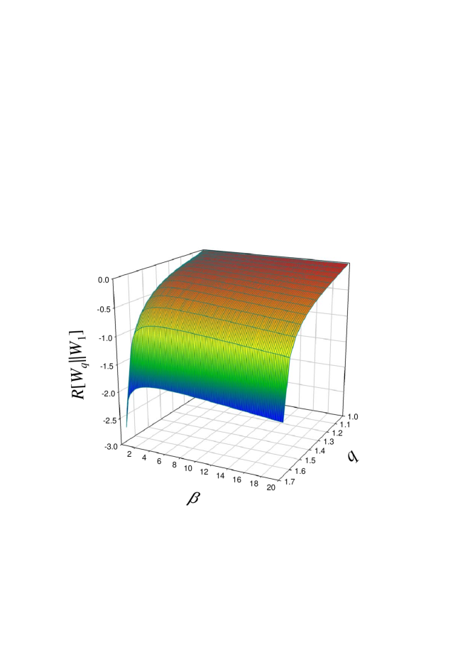
Figure 1: The renormalized entropy $\Re[W_{q}\|\widetilde{W}_{1}]$ in Eq. (III) is plotted in the interval $1<q<\frac{5}{3}$ for a representative range of $\beta$, from which the negativity of the renormalized entropy is evident.

References

- (1) F. Bardou, J. P. Bouchaud, O. Emile, A Aspect, and C. Cohen-Tannoudji, Phys. Rev. Lett. 72, 203 (1994).
- (2) C. -K. Peng, J. Mietus, J. M. Hausdorff, S. Havlin, H. E. Stanley, and A. L. Goldberger, Phys. Rev. Lett. 70, 1343 (1993).
- (3) X. Brokmann, J.P. Hermier, G. Messin, P. Desbiolles, J. -P. Bouchaud, and M. Dahan, Phys. Rev. Lett. 90, 120601 (2003).
- (4) R. Soller and S. A. Koehler, Phys. Rev. Lett. 100, 208301 (2008).
- (5) Sergio Picozzi and Bruce J. West, Phys. Rev. E 66, 046118 (2002).
- (6) D. Sornette, C. Vanneste, and L. Knopoff, Phys. Rev. A 45, 8351 (1992).
- (7) C. Tsallis, J.Stat. Phys. 52, 479 (1988).
- (8) For a recent review, see M. Gell-Mann and C. Tsallis, eds., Nonextensive Entropy - Interdisciplinary Applications (Oxford University Press, New York, 2004); J.P. Boon and C. Tsallis, eds., Nonextensive Statistical Mechanics: New Trends, New perspectives, Europhysics News 36 (6) (European Physical Society, 2005).
- (9) Eric Lutz, Phys. Rev. A 67, 051402(R) (2003).
- (10) P. Douglas, S. Bergamini, and F. Renzoni, Phys. Rev. Lett. 96, 110601 (2006).
- (11) G. Grynberg and C. Robilliard, Phys. Rep. 355, 335 (2001).
- (12) Yu. L. Klimontovich, Z. Phys. B 66, 125 (1987).
- (13) Yu. L. Klimontovich, Chaos, Solitons and Fractals 5, 1985 (1994).
- (14) Yu. L. Klimontovich, Physica A 142, 390 (1987).
- (15) Yu. L. Klimontovich, Turbulent Motion and the Structure of Chaos: A New Approach to the Statistical Theory of Open System (Kluwer Academic Publishers, Dordrecht, 1991).
- (16) Yu. L. Klimontovich, Physica Scripta 58, 549 (1998).
- (17) Yu. L. Klimontovich and M. Bonitz, Z. Phys. B 70, 241 (1988).
- (18) J. W. Gibbs, Elementary Principles in Statistical Mechanics (Yale University Press, New York, 1992).
- (19) H. Haken, Information and Self-organization: A Macroscopic Approach to Complex Systems (Springer Verlag, Berlin, 2000).
- (20) P. Saparin, A. Witt, J. Kurths, V. Anischenko, Chaos, Solitons and Fractals4, 1907 (1994).
- (21) J. Kurths et al., Chaos 5, 88 (1995).
- (22) A. Voss et al., Cardiovasc. Res. 31, 419 (1996).
- (23) K. Kopitzki, P. C. Warnke, J. Timmer, Phys. Rev. E 58, 4859 (1998).
- (24) G. B. Bağcı, Int.J. Mod. Phys. B 22, 3381 (2008).
- (25) G. B. Bağcı and U. Tirnakli, Self-organization in nonadditive systems with external noise, arXiv: 0812. 0949.
- (26) R. Gray, Entropy and Information Entropy (Springer-Verlag, New York, 1990).
- (27) R. Q. Quiroga, J. Arnold, K. Lehnertz, P. Grassberger, Phys. Rev. E 62, 8380 (2000).
- (28) S. Abe and G. B. Bağcı, Phys. Rev. E 71, 016139 (2005).
- (29) S. Abe, Phys. Rev. E 66, 046134 (2002).
- (30) Y. Castin, J. Dalibard, and C. Cohen-Tannoudji, in Light Induced Kinetic effects on Atoms, Ions and Molecules, edited by L Moi et al. (ETS Editrice, Pisa, 1991).
- (31) T. W. Hodapp, C. Gerz, C. Furtlehner, C. I. Westbrook, W. D. Phillips, and J. Dalibard, Appl. Phys. B: Lasers Opt. B60, 135 (1995).
- (32) S. Marksteiner, K. Ellinger, and P. Zoller, Phys. Rev. A 53, 3409 (1996).
- (33) L. Borland, Phys. Lett. A 245, 67 (1998).
- (34) I. S Gradshteyn and I. M. Ryzhik, Table of Integrals, Series, and Products (Academic Press, California, 2000).
- (35) C. Cohen-Tannoudji, Rev. Mod. Phys. 70, 707 (1998).
- (36) A. G. Bashkirov and A. V. Vityazev, Physica A 277, 136 (2000).
- (37) A. Rényi, Probability Theory (North-Holland, Amsterdam, 1970).