ABSTRACT

During the last few years the Tevatron has dramatically improved the bounds on rare $B$-meson decays into two leptons. In the case of $B_{s}^{0}\rightarrow\mu^{+}\mu^{-}$, the current bound is only ten times greater than the Standard Model expectation. Sensitivity to this decay is one of the benchmark goals for LHCb performance and physics. The Higgs penguin dominates this rate in the region of large $\tan\beta$ of the MSSM. This is not necessarily the case in the region of low $\tan\beta$, since box and $Z$-penguin diagrams may contribute at a comparable rate. In this article, we compute the complete one-loop MSSM contribution to $B_{s,d}^{0}\rightarrow\ell^{+}\ell^{\prime-}$ for $\ell,\ell^{\prime}=e,\mu$. We study the predictions for general values of $\tan\beta$ with arbitrary flavour mixing parameters. We discuss the possibility of both enhancing and suppressing the branching ratios relative to their Standard Model expectations. In particular, we find that there are “cancellation regions” in parameter space where the branching ratio is suppressed well below the Standard Model expectation, making it effectively invisible to the LHC.

1 Introduction

One of the most promising signals for new physics at the LHC is the rare decay $B^{0}_{s}\rightarrow\mu^{+}\mu^{-}$. This decay is suppressed as a loop-level flavour-changing neutral current and by a lepton mass insertion required for the final state muon helicities. The LHC will be the first experiment to be able to probe this decay channel all the way down to its Standard Model (SM) branching ratio. The decay is especially ‘clean’ because its final state is easily tagged and its only hadronic uncertainties come from the hadronic decay constant $f_{B_{s}}$. Further, enhancements to this branching ratio by new physics can be resolved with only a few inverse femtobarns of data, making this an exciting channel for beyond the standard model searches in the first few years of LHC operation.

The current experimental status and the Standard Model predictions for the branching ratios $\mathcal{B}(B_{s,d}^{0}\rightarrow\ell^{+}\ell^{\prime-})$ to leading order in QCD are displayed in Table 1. This is the updated version of the Table 1 presented in the review of Ref. [1]. Further reviews can be found in Ref. [2].

Channel	Expt.	Bound (90% CL)	SM Prediction
$B^{0}_{s}\to\mu^{+}\mu^{-}$	CDF II [3]	$<4.7\times 10^{-8}$	$(4.8\pm 1.3)\times 10^{-9}$
$B^{0}_{d}\to\mu^{+}\mu^{-}$	CDF II [3]	$<1.5\times 10^{-8}$	$(1.4\pm 0.4)\times 10^{-10}$
$B^{0}_{s}\to\mu^{+}e^{-}$	CDF [4]	$<6.1\times 10^{-6}$	$\approx 0$
$B^{0}_{d}\to\mu^{+}e^{-}$	BABAR [5]	$<9.2\times 10^{-8}$	$\approx 0$

Table 1: Current experimental bounds and SM expectations for leptonic $B^{0}$-meson decays.

The Standard Model predictions for the dimuon decay of $B^{0}_{s}$ and $B^{0}_{d}$ mesons were first calculated by Buchalla and Buras in Ref. [6] and Higgs penguin contributions in Ref. [7]. Their analysis can be generalised to include lepton flavour-violating decays with the final state $\mu^{+}e^{-}$ which are not measurable within the SM extended with see-saw neutrino masses. The error in the SM predictions for the $B_{s,d}$ branching ratios originates primarily from the uncertainties in the decay constants [8],

$$f_{B_{s}}=230\pm 30\hskip 5.69046pt\mathrm{MeV}\;,\qquad f_{B_{d}}=200\pm 30\hskip 5.69046pt\mathrm{MeV}\;,$$ (1.1)

and in the top-strange and top-down elements of the Cabibbo-Kobayashi-Maskawa (CKM) matrix [9],

$$|V_{ts}|=0.0406\pm 0.0027\;,\qquad|V_{td}|=0.0074\pm 0.0008\;.$$ (1.2)

The dimuon decay of $B^{0}_{s}$ is of particular interest to experimentalists because it is a benchmark process for LHCb physics and performance. The LHCb will be able to directly probe the SM predictions for this rare decay mode at $3\sigma$ ($5\sigma$) significance with 2 $\mathrm{fb}^{-1}$ (6 $\mathrm{fb}^{-1}$) of data, or after about one year (three years) of design luminosity [10]. In addition, the general purpose detectors ATLAS and CMS will also be able to reconstruct the $B_{s}^{0}\rightarrow\mu^{+}\mu^{-}$ signal with significance of $3\sigma$ after $\approx$ 30 $\mathrm{fb}^{-1}$ [11]. It is not clear whether LHC can reach the SM expectation for $B_{d}^{0}\rightarrow\mu^{+}\mu^{-}$.

At the dawn of the LHC era, it is important to understand the possible contributions of new physics to a discovery in the $B^{0}_{s,d}\rightarrow\ell^{+}\ell^{\prime-}$ channels. These are particularly promising decay channels for the Minimal Supersymmetric Standard Model (MSSM). Under the assumption of large values of $\tan\beta$ and Minimal Flavour Violation (MFV), where the CKM matrix is the only source of $CP$ and flavour violation, the branching ratio for $B^{0}_{s}\rightarrow\mu^{+}\mu^{-}$ is dominated by the Higgs penguin mode and is approximately given by

$${\cal B}(B^{0}_{s}\rightarrow\mu^{+}\mu^{-}) \approx 5\cdot 10^{-7}\left(\frac{\tan\beta}{50}\right)^{6}\left(\frac{300\hskip 5.69046pt\mathrm{GeV}}{M_{A}}\right)^{4}\;,$$ (1.3)

where $M_{A}$ is the $CP$-odd Higgs mass. Thus in the large $\tan\beta$ regime this branching ratio can be significantly enhanced over the Standard Model expectation. This has been discussed extensively in Refs. [12, 13, 14, 15, 1]. The large $\tan\beta$ regime is preferred, for example, by supersymmetric $SO(10)$ grand unified models. Further, the currently observed excess in the anomalous magnetic moment of the muon $(g-2)_{\mu}$ [16] implies an additional enhancement in $\mathcal{B}(B_{s}^{0}\rightarrow\mu^{+}\mu^{-})$ in certain supergravity scenarios [17]. A field theoretic study of this decay in the large $\tan\beta$ limit focusing on the resummation of $\tan\beta$ was conducted in Ref. [18, 19, 20, 21].

Thus far, however, the published analyses have focused primarily on the large $\tan\beta$ region with MFV and have neglected possible flavour mixing in the squark sector. With the upcoming experimental probes of $\mathcal{B}(B^{0}_{s,d}\rightarrow\ell^{+}\ell^{\prime-})$ down to the SM expectation, it is important to undertake a full, general calculation of this branching ratio without a priori assumptions on the pattern of squark and slepton flavour mixing or electroweak symmetry breaking. In particular, in the region of low $\tan\beta$, the effects of box and $Z$-penguin diagrams could be of the same order as the $\tan\beta$-enhanced Higgs penguins. The interference of these terms could conceivably lead to a cancellation that would suppress the branching ratio below the SM prediction. This region of parameter space has not yet been thoroughly investigated. This paper fills the gap in the literature on the low $\tan\beta$ properties of these decay modes.

If the branching ratio is significantly enhanced by new physics, it may even be visible at the Tevatron. Alternately, if it is significantly suppressed by new physics, it may be invisible even at the LHC. Either way, the status of this decay could become an important factor for planned LHCb upgrades. For example, it could play a critical role in determining whether an LHCb upgrade should focus on a more precise measurement of $B_{s}^{0}\rightarrow\mu^{+}\mu^{-}$ or instead reach for the branching ratio of $B_{d}^{0}\rightarrow\mu^{+}\mu^{-}$ which is an order of magnitude smaller.

In this article we calculate MSSM predictions for dileptonic $B_{d},B_{s}$ decays with arbitrary flavour mixing. In our numerical analysis, we ignore $\tau$-lepton final states since decays like $B_{s}^{0}\rightarrow{}\tau^{+}\tau^{-}$ or $B_{s}^{0}\rightarrow\tau^{+}\mu^{-}$ since they cannot be observed accurately at the Tevatron or LHC. Although our calculation is sufficiently general to include lepton flavour violating $B$-decays like $B^{0}\to\mu^{\pm}e^{\mp}$, we do not consider them in our numerical analysis due to their small branching ratio ($\raisebox{-3.69899pt}{~{}\shortstack{$<$\\ [-0.07cm] $\sim$}}~{}10^{-11}$) at low $\tan\beta$. We therefore concentrate on the decays $B_{s}^{0}\rightarrow\mu^{+}\mu^{-}$ and $B_{d}^{0}\rightarrow\mu^{+}\mu^{-}$. The general calculation is presented in the appendix and the code used in our numerical analysis is available to the public.

2 Effective Operators and Branching Ratios

There are ten effective operators governing the dynamics of the quarks-to-leptons transition $q^{I}q^{J}\rightarrow\ell^{+K}\,\ell^{-L}$, with $q^{1}\equiv d,q^{2}\equiv s,q^{3}\equiv b$ and $\ell^{1}\equiv e,\ell^{2}\equiv\mu,\ell^{3}\equiv\tau$. The effective Hamiltonian reads:

$${\cal H}\ =\ \frac{1}{(4\pi)^{2}}\sum_{X,Y=L,R}\biggl{(}C_{VXY}\,\mathcal{O}_{VXY}\ +\ C_{SXY}\,\mathcal{O}_{SXY}\ +\ C_{TX}\,\mathcal{O}_{TX}\biggr{)}\;,$$ (2.1)

where flavour and colour indices have been suppressed for brevity. The (V)ector, (S)calar and (T)ensor operators are respectively given by

$$\mathcal{O}_{VXY}^{IJKL}\ = \ (\overline{q^{J}}\,\gamma^{\mu}\,P_{X}\,q^{I})(\overline{\ell^{L}}\,\gamma_{\mu}\,P_{Y}\,\ell^{K})\;,$$

$$\mathcal{O}_{SXY}^{IJKL}\ = \ (\overline{q^{J}}\,P_{X}\,q^{I})(\overline{\ell^{L}}\,P_{Y}\,\ell^{K})\;,$$

$$\mathcal{O}_{TX}^{IJKL}\ = \ (\overline{q^{J}}\sigma^{\mu\nu}\,P_{X}\,q^{I})(\overline{\ell^{L}}\,\sigma_{\mu\nu}\,\ell^{K})\;.$$ (2.2)

We follow the PDG conventions for the quark content of the $B^{0}$-mesons, $B_{s}^{0}\equiv\overline{b}s$ and $B_{d}^{0}\equiv\overline{b}d$ [23]. Thus in Eq. (2.2) we identify $q^{J}\equiv b$ and $q^{I}\equiv s$ or $d$ for $B_{s,d}^{0}\rightarrow\ell^{+}\ell^{\prime-}$ respectively.

The explicit forms of the Wilson coefficients for the MSSM are calculated at the electroweak scale, $Q=M_{W}$. These are given in the appendix. The contributions to these coefficients can be classified into $Z$-penguins, Higgs-penguins and box diagrams, shown in Fig. 1. The photon penguin contribution $B_{s}^{0}\rightarrow\ell^{+}\ell^{\prime-}$ vanishes in matrix element calculations due to the Ward identity. We do not consider the very large $\tan\beta$ scenario ($\tan\beta\raisebox{-3.69899pt}{~{}\shortstack{$>$\\ [-0.07cm] $\sim$}}~{}30$), since in this region our calculation has nothing to add to the current literature (see previous section for references). Thus no resummation of higher orders in $\tan\beta$ is necessary and all formulae given in the appendix are strictly one-loop.

Figure 1: Diagrams contributing to $q^{I}q^{J}\rightarrow l^{K}l^{L}$ transitions.

We now focus on the decay $B_{s}^{0}\rightarrow\ell^{+K}\,\ell^{-L}$. Corresponding formulae for the $B_{d}^{0}$ decays can be derived analogously. Down quark vector and scalar currents hadronize to $B_{s}$-mesons as

$$\langle 0|\overline{b}\gamma_{\mu}P_{L(R)}s|B_{s}(p)\rangle\ = \ -(+)\frac{i}{2}p_{\mu}f_{B_{s}}\;,$$ (2.3)

$$\langle 0|\overline{b}P_{L(R)}s|B_{s}(p)\rangle\ = \ +(-)\frac{i}{2}\,\frac{M_{B_{s}}^{2}f_{B_{s}}}{m_{b}+m_{s}}\;.$$ (2.4)

where $p_{\mu}=p_{1\mu}+p_{3\mu}$ is the momentum of the decaying $B_{s}$-meson of mass $M_{B_{s}}$. In deriving Eq. (2.4) we have used the quark equations of motion. One immediate consequence of the $B_{s}^{0}\rightarrow\ell^{+}\ell^{\prime-}$ kinematics is that tensor operators vanish in the matrix element $\langle 0|\overline{b}\,\sigma_{\mu\nu}\,s|B_{s}(p)\rangle$ because there is no way to make an antisymmetric tensor with the single available momentum $p_{\mu}$. This reduces the total number of effective operators contributing to $B_{s}^{0}\rightarrow\ell^{+}\ell^{\prime-}$ in Eq. (2.2) from ten to eight. The matrix element is therefore

$$\mathcal{M}\ =\ F_{S}\,\overline{\ell}\ell\ +\ F_{P}\,\overline{\ell}\gamma_{5}\ell\ +\ F_{V}\,p^{\mu}\overline{\ell}\gamma_{\mu}\ell\ +\ F_{A}\,p^{\mu}\overline{\ell}\gamma_{\mu}\gamma_{5}\ell\;,$$ (2.5)

where the $\ell$s correspond to external lepton spinors, e.g. $F_{S}\,\overline{\ell}\ell\equiv F_{S\,}\overline{u}(p_{2})\,v(p_{4})$, etc. The momenta are assigned as in Fig. 1. The (S)calar, (P)seudoscalar, (V)ector and (A)xial-vector form factors in Eq. (2.5) are given by

$$F_{S}\ = \ \frac{i}{4}\,\frac{M_{B_{s}}^{2}f_{B_{s}}}{m_{b}+m_{s}}\;(C_{SLL}+C_{SLR}-C_{SRR}-C_{SRL})\;,$$ (2.6)

$$F_{P}\ = \ \frac{i}{4}\,\frac{M_{B_{s}}^{2}f_{B_{s}}}{m_{b}+m_{s}}\;(-C_{SLL}+C_{SLR}-C_{SRR}+C_{SRL})\;,$$ (2.7)

$$F_{V}\ = \ -\frac{i}{4}f_{B_{s}}\;(C_{VLL}+C_{VLR}-C_{VRR}-C_{VRL})\;,$$ (2.8)

$$F_{A}\ = \ -\frac{i}{4}f_{B_{s}}\;(-C_{VLL}+C_{VLR}-C_{VRR}+C_{VRL})\;.$$ (2.9)

It is now straightforward to square the matrix element in Eq. (2.5), and determine the branching ratio for the decay $B_{s}^{0}\rightarrow\ell^{+}\ell^{\prime-}$,

$$\mathcal{B}(B_{s}^{0}\rightarrow\ell_{L}^{-}\,\ell_{K}^{+})\ =\ \frac{\tau_{B_{s}}}{16\pi}\,\frac{|\mathcal{M}|^{2}}{M_{B_{s}}}\,\sqrt{1-\biggl{(}\frac{m_{\ell_{K}}+m_{\ell_{L}}}{M_{B_{s}}}\biggr{)}^{2}}\,\sqrt{1-\biggl{(}\frac{m_{\ell_{K}}-m_{\ell_{L}}}{M_{B_{s}}}\biggr{)}^{2}}\;,$$ (2.10)

where $\tau_{B_{s}}$ is the lifetime of $B_{s}$ meson, and

$$(4\pi)^{4}|\mathcal{M}|^{2} = 2|F_{S}|^{2}\left[M_{B_{s}}^{2}-(m_{\ell_{L}}+m_{\ell_{K}})^{2}\right]\ +\ 2|F_{P}|^{2}\left[M_{B_{s}}^{2}-(m_{\ell_{L}}-m_{\ell_{K}})^{2}\right]$$ (2.11)

$$+ 2|F_{V}|^{2}\left[M_{B_{s}}^{2}(m_{\ell_{K}}-m_{\ell_{L}})^{2}-(m_{\ell_{K}}^{2}-m_{\ell_{L}}^{2})^{2}\right]$$

$$+ 2|F_{A}|^{2}\left[M_{B_{s}}^{2}(m_{\ell_{K}}+m_{\ell_{L}})^{2}-(m_{\ell_{K}}^{2}-m_{\ell_{L}}^{2})^{2}\right]$$

$$+ 4\,\mathrm{Re}(F_{S}F_{V}^{*})(m_{\ell_{L}}-m_{\ell_{K}})\left[M_{B_{s}}^{2}+(m_{\ell_{K}}+m_{\ell_{L}})^{2}\right]$$

$$+ 4\,\mathrm{Re}(F_{P}F_{A}^{*})(m_{\ell_{L}}+m_{\ell_{K}})\left[M_{B_{s}}^{2}-(m_{\ell_{L}}-m_{\ell_{K}})^{2}\right]\;.$$

Notice that the contribution from the vector amplitude, $F_{V}$, vanishes in the lepton flavour conserving case, $L=K$. In this case the formula in Eq. (2.11) agrees with results of Ref. [24].

The form factors in Eqs. (2.6 – 2.9) do not receive additional renormalisation due to QCD corrections. The conservation of axial-vector current operators ($\mathcal{O}_{VXY}$) result in vanishing anomalous dimension associated with this operator. The scalar operators ($\mathcal{O}_{SXY}$) renormalise like a quark mass parameter and thus the ratio $C_{SXY}(Q)/[m_{b}(Q)+m_{s}(Q)]$ is a renormalisation group invariant quantity [25].

Wilson coefficients and parameters entering Eqs. (2.6 – 2.9) and (2.11) are all calculated at the top quark mass scale, i.e. $Q=m_{t}$. The quark pole masses, $m_{b}$ or $m_{t}$, are related to their $\overline{DR}$-running one-loop quark masses at the scale $Q$, $m_{q}(Q)$, by the well-known formulae:

$$m_{b}(Q)\ = \ m_{b}\,\biggl{[}1-\frac{5\,\alpha_{s}(m_{b})}{3\pi}\biggr{]}\,\biggl{[}\frac{\alpha_{s}(Q)}{\alpha_{s}(m_{b})}\biggr{]}^{\frac{4}{b_{0}}}\;,$$ (2.12)

$$m_{t}(m_{t})\ = \ m_{t}\,\biggl{[}1-\frac{5\,\alpha_{s}(m_{t})}{3\pi}\biggr{]}\;,$$ (2.13)

with $b_{0}=11-2n_{f}/3$ with $n_{f}=5$. Since our calculation for the SUSY corrections is performed in the $\overline{DR}$ renormalization scheme [26], our initial conditions for parameters must be converted into this scheme. Eqs. (2.12) and (2.13) contain the appropriate $\overline{MS}\longrightarrow\overline{DR}$ conversion factors [27]. Similar conversions for gauge couplings is small and is ignored in our numerical results.

We have included the general decays of Eq. (2.10) in our numerical code. Due to small branching ratios, however, it is unlikely that we will observe lepton flavour violating $B$-meson decays at moderate or small values of $\tan\beta$ and so we will not consider these processes in the remainder of this paper.

3 Numerical Analysis of $B_{s,d}\rightarrow\mu^{+}\mu^{-}$

3.1 Structure of the MSSM contributions

We now focus on the lepton flavour-conserving processes $B_{s,d}^{0}\rightarrow\mu^{+}\mu^{-}$. Recall from Section  1 that we are interested in cases where the branching ratios for these processes are either enhanced or suppressed significantly relative to their Standard Model predictions. An enhancement would either lead to an early discovery at the LHC (or even the Tevatron) or stronger constraints on the allowed magnitude of squark flavour violation. A suppression, on the other hand, could lead to a non-observation of $B_{s}^{0}\rightarrow\mu^{+}\mu^{-}$ at the LHCb due to cancellations from new physics in the decay amplitude.

For the lepton flavour conserving decays $\ell_{K}=\ell_{L}=\mu$ and the squared amplitude in Eq. (2.11) takes the form

$$|\mathcal{M}|^{2}\approx\frac{2M_{B_{q}}^{2}}{(16\pi^{2})^{2}}\left(|F_{S}|^{2}\ +\ |F_{P}+2\,m_{\mu}\,F_{A}|^{2}\right)\;,$$ (3.1)

where we have also taken the limit $m_{\mu}/M_{B_{q}}\to 0$. We may distinguish two possible scenarios for the relative size of the MSSM contributions to the right-hand side of Eq. (3.1):

• Higgs penguin domination or large $\tan\beta\raisebox{-3.69899pt}{~{}\shortstack{$>$\\ [-0.07cm] $\sim$}}~{}10$

  In this large $\tan\beta$ regime one can usually expect an enhancement of the branching ratios as in Eq. (1.3). This case has been thoroughly investigated in the literature, although mostly in the limit of minimal flavour violation and vanishing intergenerational squark mixing. In such case it turns out that $|F_{S}|\approx|F_{P}|\gg 2m_{\ell}|F_{A}|$ because of $\tan^{2}\beta$ enhancements. Although this is the standard situation for large $\tan\beta$, it is not general since a kind of Glashow -Iliopoulos -Maiani (GIM) cancellation mechanism may result in $F_{S,P}^{\rm SUSY}\approx 0$  [18, 21], thus making the box and $Z$-penguin diagrams phenomenologically relevant.

• Comparable Box, $Z$-penguin and Higgs penguin contributions or low $\tan\beta\raisebox{-3.69899pt}{~{}\shortstack{$<$\\ [-0.07cm] $\sim$}}~{}10$

  In this low $\tan\beta$ case the supersymmetric Higgs-mediated form factors $F_{S,P}$ are suppressed and become comparable to or even smaller than $F_{A}$. Thus the full one-loop corrections to the amplitude are needed. These are presented in the appendix. In this case either an enhancement or a suppression of the branching ratios is possible depending on the particular choice of MSSM parameters.

Barring accidental cancellations, an enhancement of the branching ratios can come from any of the contributions in Fig. 1. On the other hand, it is a bit trickier to suppress the branching ratios below their Standard Model predictions as this requires a cancellation between various terms. This is the case we would like to investigate further.

We would like to find the minima of $\mathcal{B}(B_{s,d}^{0}\rightarrow\mu^{+}\mu^{-})$, i.e. the minima of Eq. (3.1). We distinguish between two cases:

$$F_{P}+2\,m_{\ell}\,F_{A}\approx 0\qquad\mathrm{and}\qquad F_{P}\gg F_{S}\;,$$ (3.2)

$$\mathrm{or}$$

$$|F_{S}|\,\approx\,|F_{P}|\,\approx\,|F_{A}|\approx 0\;.$$ (3.3)

In the first case, Eq. (3.2), the pseudoscalar and axial contributions cancel while the scalar contribution is negligible. This can be realized, for example, in models where the MSSM is extended with an additional, light, $CP$-odd Higgs boson. Ref. [28] shows that this can occur even in the minimal flavour violating limit of such a model. Such cancellations, however, can also take place in the general MSSM when left- and right-handed squarks mix in the strange and charm sectors. Furthrmore, it has been pointed out in Ref. [29], that interference between the scalar/pseudoscalar new physics and Standard Model operators can decrease the $\mathcal{B}(B_{s}^{0}\rightarrow\mu^{+}\mu^{-})$ far below its SM prediction. This is explored further within MSSM in the numerical analysis of Section 3.2.

The second case, Eq. (3.3), happens when Higgs contributions are negligible compared to the axial contribution (i.e. low $\tan\beta$ and large $M_{A}$) and $F_{A}$ becomes small due to cancellations among the $C_{VXY}$ coefficients in Eq. (2.8). Our numerical analysis shows that such a cancellation is possible but requires a certain amount of fine tuning once constraints on squark mass insertions from other flavour-changing neutral current (FCNC) measurements are imposed.

3.2 Numerical setup

To quantitatively study the effects mentioned in the previous section, we perform a scan over the MSSM parameter space. The ranges of variation over MSSM parameters are shown in Table 2. Because our numerical analysis is based on the general calculation presented in the previous section, we are not restricted to particular values of $\tan\beta$ or the MFV scenario. Flavour violation is parameterised by the “mass insertions”, defined as in [30, 31],

$$\delta^{IJ}_{QXY} = \frac{(M^{2}_{Q})^{IJ}_{XY}}{\sqrt{(M^{2}_{Q})^{IJ}_{XX}(M^{2}_{Q})^{IJ}_{YY}}}\;.$$ (3.4)

As before, $I,J$ denote quark flavours, $X,Y$ denote superfield chirality, and $Q$ indicates either the up or down quark superfield sector.

Parameter	Symbol	Min	Max	Step
Ratio of Higgs vevs	$\tan\beta$	2	30	varied
CKM phase	$\gamma$	$0$	$\pi$	$\pi/25$
CP-odd Higgs mass	$M_{A}$	100	500	200
SUSY Higgs mixing	$\mu$	-450	450	300
$SU(2)$ gaugino mass	$M_{2}$	100	500	200
Gluino mass	$M_{3}$	$3M_{2}$	$3M_{2}$	0
SUSY scale	$M_{\mathrm{SUSY}}$	500	1000	500
Slepton Masses	$M_{\tilde{\ell}}$	$M_{\mathrm{SUSY}}/3$	$M_{\mathrm{SUSY}}/3$	0
Left top squark mass	$M_{\tilde{Q}_{L}}$	200	500	300
Right bottom squark mass	$M_{\tilde{b}_{R}}$	200	500	300
Right top squark mass	$M_{\tilde{t}_{R}}$	150	300	150
Mass insertion	$\delta_{dLL}^{13}$, $\delta_{dLL}^{23}$	-1	1	1/10
Mass insertion	$\delta_{dLR}^{13}$, $\delta_{dLR}^{23}$	-0.1	0.1	1/100

Table 2: The range of input parameters for the numerical scan. “SUSY scale” refers to the common mass parameter for the first two squark generations. The parameter $\tan\beta$ takes on values within the set: $\tan\beta=(2,4,6,8,10,13,16,19,22,25,30)$. All mass parameters are in GeV. The top quark pole mass have been taken 171 GeV. Imaginary part of parameters $\delta_{dLL}^{IJ}$, $\delta_{dLR}^{IJ},\mu$ and $M_{2}$ have been set to zero. The trilinear soft SUSY breaking couplings are set to $A_{t}=A_{b}=M_{\tilde{Q}_{L}}$ and $A_{\tilde{\tau}}=M_{\tilde{\ell}}$ throughout.

To realistically estimate the allowed range for $\mathcal{B}(B_{s,d}^{0}\rightarrow\mu^{+}\mu^{-})$, one must account the experimental constraints from measurements of many other rare decays. SUSY mass insertions, in particular, are strongly constrained by such measurements. The most important constraints have been calculated in the framework of the general MSSM using a standard set of conventions [31, 32, 33, 34, 35, 19, 36]. We have used the library of numerical codes developed in those studies to bound the MSSM parameter space based on the set of observables listed in Table 3; no further bounds (e.g. dark matter, electroweak observables, etc.) are imposed other than those listed.

For all the quantities in Table 3 for which the experimental result and its error are known, we require

$$|Q^{exp}-Q^{th}|\leq 3\Delta Q^{exp}+q|Q^{th}|.$$ (3.5)

For the quantities for which only the upper bound is known, we require

$$(1+q)|Q^{th}|\leq Q^{exp}.$$ (3.6)

Quantity	Current Measurement	Experimental Error
$m_{\chi^{0}_{1}}$	$>$ 46  GeV
$m_{\chi^{\pm}_{1}}$	$>$ 94  GeV
$m_{\tilde{b}}$	$>$ 89  GeV
$m_{\tilde{t}}$	$>$ 95.7 GeV
$m_{h}$	$>$ 92.8  GeV
$|\epsilon_{K}|$	$2.232\cdot 10^{-3}$	$0.007\cdot 10^{-3}$
$|\Delta M_{K}|$	$3.483\cdot 10^{-15}$	$0.006\cdot 10^{-15}$
$|\Delta M_{D}|$	$<0.46\cdot 10^{-13}$
$\Delta M_{B_{d}}$	$3.337\cdot 10^{-13}~{}{\rm GeV}$	$0.033\cdot 10^{-13}~{}{\rm GeV}$
$\Delta M_{B_{s}}$	$116.96\cdot 10^{-13}~{}{\rm GeV}$	$0.79\cdot 10^{-13}~{}{\rm GeV}$
Br($B\rightarrow X_{s}\gamma$)	$3.34\cdot 10^{-4}$	$0.38\cdot 10^{-4}$
Br($K_{L}\rightarrow\pi^{0}\nu\bar{\nu}$)	$<1.5\cdot 10^{-10}$
Br($K^{+}\rightarrow\pi^{+}\nu\bar{\nu}$)	$1.5\cdot 10^{-10}$	$1.3\cdot 10^{-10}$
Electron EDM	$<0.07\cdot 10^{-26}$
Neutron EDM	$<0.63\cdot 10^{-25}$

Table 3: Constraints used in the scan over MSSM parameters. LEP data are used for the Higgs mass bound [37], i.e. $m_{h}\geq 92.8-114$ GeV depending on the value of $\sin^{2}(\alpha-\beta)$.

The first and second terms on the right-hand side of Eq. (3.5) represent the $3\sigma$ experimental error and the theoretical error respectively. The latter differs from quantity to quantity and is usually smaller than the value $q=50\%$ which we assume generically in all calculations. Apart from the theoretical errors that come from uncertainties in the QCD evolution and hadronic matrix elements, one must also take into account the limited density of a numerical scan. In principle, with a very dense scan and sufficient computing time, it should be possible to find SUSY parameters that fulfill Eq. (3.5) within the calculation’s “true” theoretical errors. This, however, may not be necessary and may even be undesirable. Our goal is to find “generic” values for the branching ratio $\mathcal{B}(B_{s,d}^{0}\rightarrow\mu^{+}\mu^{-})$, i.e. values allowed by fairly wide ranges of SUSY parameters without strong fine tuning or the need to resort to special points in parameter space where “miraculous” cancellations evade experimental bounds. In our scan we thus use wide “theoretical” errors assuming that this procedure faithfully represents the ranges of the MSSM parameters. If necessary the exact values of parameters fulfilling the bound in Eq. (3.5) with smaller $q$ can be found. A more detailed discussion of the problems associated with scanning over multidimensional MSSM parameter space can be found in [36].

3.3 Predictions for ${\mathcal{B}}(B_{s}\to\mu^{+}\mu^{-})$

Fig. 2 shows the predictions for $\mathcal{B}(B_{s}^{0}\rightarrow\mu^{+}\mu^{-})$ over a general scan of 20 million points in parameter space according to Table 3 and including the bounds described in the previous section. The upper bound set by CDF in Table 1, depicted as a solid red line, can be attained even with very low values of $\tan\beta$. We focus on the lower limit of the branching ratio and therefore restrict to the region of parameter space where $\tan\beta\raisebox{-3.69899pt}{~{}\shortstack{$<$\\ [-0.07cm] $\sim$}}~{}30$. In this way we also avoid the technical complications connected with the resummation of higher order terms, discussed in Refs. [18, 19, 20, 21]. We vary $\delta_{d\,LL}^{23}$ (upper panel) and $\delta_{d\,LR}^{23}$ (lower panel) one at a time while setting the other to zero, e.g. all $\delta_{XY}^{{ij}}=0$ and only $\delta_{d\,LL}^{23}\neq 0$ in the upper panel.

When $\delta_{d\,LL}^{23}$ is varied in the range $[-1,1]$, we find $\mathcal{B}(B_{s}^{0}\rightarrow\mu^{+}\mu^{-})_{min}\approx 10^{-9}$. This minimum is almost independent of $\tan\beta$ but depends on the magnitude of the mass insertion (upper right panel). $|\delta_{d\,LL}^{23}|$ can take on values up to $\approx 0.9$ and still pass all the constraints in Table 3, though points beyond $0.3$ are less dense. We note here the importance of correctly incorporating the LEP Higgs mass bound. If for example we set $m_{h}>114$ GeV independently of the value of the $ZZH$ coupling, then $|\delta_{d\,LL}^{23}|$ is restricted to values smaller than $\approx 0.3$.

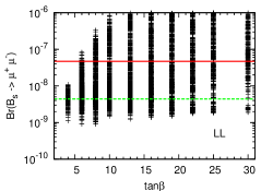
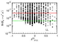
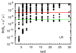
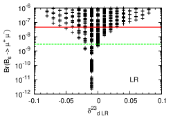
Figure 2: Upper panel: Predictions for ${\mathcal{B}}(B_{s}\to\mu^{+}\mu^{-})$ versus $\tan\beta$ (left) and $\delta_{d\,LL}^{23}$ (right) from the scan of MSSM parameters in Table 2 and under the constraints of Table 3. The upper solid line shows the current upper bound from the Tevatron and the lower dashed line the SM expectation. Lower panel: Similar to the upper panel but with $\delta_{d\,LR}^{23}$ varied.

More interesting is the case when $\delta_{d\,LR}^{23}$ is varied in the range $[-0.1,0.1]$. We find a narrow cancellation region around $\delta_{d\,LR}^{23}\approx-0.01$ and $\tan\beta\raisebox{-3.69899pt}{~{}\shortstack{$<$\\ [-0.07cm] $\sim$}}~{}10$ where $\mathcal{B}(B_{s}^{0}\rightarrow\mu^{+}\mu^{-})_{min}\approx 10^{-12}$ (lower right panel). This is three orders of magnitude lower than the Standard Model prediction, making it effectively unobservable at the LHC. In order to better understand cancellation region we study a representative point with a very low branching ratio, for example:

$$\tan\beta=4,\quad M_{A}=300,\quad\mu=-450,\quad M_{2}=100,\quad M_{3}=300,$$

$$\mathrm{SUSY~{}scale}=400,\quad M_{\tilde{t}_{R}}=150,\quad A_{t,b}=M_{\tilde{t}_{L}}=M_{\tilde{b}_{(L,R)}}=600\;,$$ (3.7)

where all masses are in GeV.

Figure 3: Contributions to $\mathcal{B}(B_{s,d}^{0}\rightarrow\mu^{+}\mu^{-})$ from various parts with the parameters in Eq. (3.7). Left: Contributions from the diagrams in Fig. 1 versus $\delta^{23}_{dLR}$. Right: Magnitude of the form factors appearing in Eqs. (2.6 – 2.9) versus $\delta^{23}_{dLR}$.

The cancellation is easy to understand if one independently considers the contributions to the branching ratio from each diagram, as shown on the left in Fig. 3. The ‘Box’, ‘Higgs’ and ‘$Z$’ lines indicate the value of $\mathcal{B}(B_{s}^{0}\rightarrow\mu^{+}\mu^{-})$ given by only the listed contribution with all others set to zero. The total prediction for $\mathcal{B}(B_{s}^{0}\rightarrow\mu^{+}\mu^{-})$ is also indicated. We observe that in the cancellation region the Higgs- and $Z$-penguin magnitudes are comparable while the box contribution is negligible. This is suggestive of a cancellation between the second and third class of diagrams in Fig. 1. To observe this cancellation we individually plot the absolute values of the form factors $F_{S,P}$ and $2m_{\mu}F_{A}$ of Eqs. (2.6 – 2.9) in the right panel of Fig. 3. At the minimum point of the total branching ratio (thick-dashed line in left panel of Fig. 3) $|F_{P}|$ is approximately equal to $|2m_{\mu}F_{A}|$ and $|F_{S}|$ is negligibly small. This can be explained from the form of Eqs. (2.6) and (2.7). If one assumes $\delta^{23}_{dLR}=\left(\delta^{32}_{dLR}\right)^{\star}$, then $C_{SLR}$ and $C_{SRL}$, the two Wilson coefficients most sensitive to the variation of $\delta^{23}_{dLR}$, have similar sizes and opposite sign and thus interfere destructively in the amplitude.

Bounds on the $\delta$ parameters governing squark flavour mixing have been presented in the literature using the mass insertion approximation (MIA). In particular, Refs. [38] and [39] bound $|\delta_{d\,LL}^{23}|\raisebox{-3.69899pt}{~{}\shortstack{$<$\\ [-0.07cm] $\sim$}}~{}0.3$ and $|\delta_{d\,LR}^{23}|\raisebox{-3.69899pt}{~{}\shortstack{$<$\\ [-0.07cm] $\sim$}}~{}0.02$ for a particular point in the parameter space, $m_{\tilde{q}}=M_{3}=350$ GeV. On the other hand, the results in Fig. 3 arise from an extensive scan of the experimentally allowed parameter space without resorting to MIA. Thus the bounds on the $\delta$s presented here are both different and more representative of the range of possibilities in the general MSSM. The results of this scan show that $\delta^{23}_{dLL}$ is still rather weakly constrained, whereas $\delta^{23}_{dLR}\raisebox{-3.69899pt}{~{}\shortstack{$<$\\ [-0.07cm] $\sim$}}~{}0.08$.

We remark here that varying $\delta^{13}_{dLL}$ or $\delta^{13}_{dLR}$ has almost no effect on $\mathcal{B}(B_{s}^{0}\rightarrow\mu^{+}\mu^{-})$ which takes values along a narrow band.

3.4 Predictions for ${\mathcal{B}}(B_{d}\to\mu^{+}\mu^{-})$

We present the corresponding MSSM predictions for ${\mathcal{B}}(B_{d}\to\mu^{+}\mu^{-})$ in Fig. 4 where $\delta_{d\,LL}^{13}$ or $\delta_{d\,LR}^{13}$ are varied instead of $\delta_{d\,LL}^{23}$ or $\delta_{d\,LR}^{23}$ along with the other SUSY parameters in Table 2. Some sequences of points disappear due to the experimental constraints given in Table 3. Note that varying $\delta^{23}_{dLL},\delta^{23}_{dLR}$ has almost no effect on $\mathcal{B}(B_{d}^{0}\rightarrow\mu^{+}\mu^{-})$.

For both cases there exist points where ${\mathcal{B}}(B_{d}\to\mu^{+}\mu^{-})$ is reduced by an order of magnitude relative to the SM. These points are more sensitive to low $\tan\beta$ in the ‘LL’ case and fall into the case of Eq. (3.3). It is also interesting to look at the the ratio ${\mathcal{B}}(B_{d}\to\mu^{+}\mu^{-})/{\mathcal{B}}(B_{s}\to\mu^{+}\mu^{-})$ versus $\delta_{d\,LL}^{13}$ and $\delta_{d\,LR}^{13}$ , plotted in the right panel of Fig. 4. Unlike the Standard Model where ${\mathcal{B}}(B_{d}\to\mu^{+}\mu^{-})/{\mathcal{B}}(B_{s}\to\mu^{+}\mu^{-})\approx|V_{td}/V_{ts}|^{2}\leq 0.03$, the MSSM can enhance this ratio by a factor of ten even for small values of $\delta^{13}_{d\,LL}$ or $\delta^{13}_{d\,LR}$. This suggests that collider searches for ${\mathcal{B}}(B_{d}\to\mu^{+}\mu^{-})$ are as important as those for ${\mathcal{B}}(B_{s}\to\mu^{+}\mu^{-})$. This observation has been already discussed in the literature [24] in the leading $\tan\beta$ approximation. On the other hand MSSM can further reduce the ratio in the ‘LL’ case by an order of magnitude due to the aforementioned cancellations in $\mathcal{B}(B_{d}^{0}\rightarrow\mu^{+}\mu^{-})$.

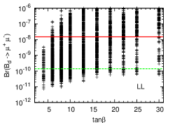
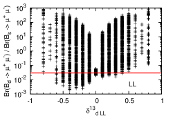
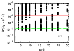
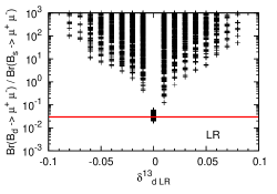
Figure 4: Upper panel: Predictions for ${\mathcal{B}}(B_{d}\to\mu^{+}\mu^{-})$ versus $\tan\beta$ (left) and ${\mathcal{B}}(B_{d}\to\mu^{+}\mu^{-})/{\mathcal{B}}(B_{s}\to\mu^{+}\mu^{-})$ versus $\delta_{d\,LL}^{13}$(right) from the scan of MSSM parameters in Table 2 and under the constraints of Table 3. The solid line shows the upper bound from the Tevatron and the dashed line shows the SM expectation. Lower panel: Similar to the upper panel but with $\delta_{d\,LR}^{13}$ varied. In all plots only the $\delta$ indicated is varied with all other mass insertions set to zero.

4 Conclusions

We have presented a complete, one-loop calculation of the branching ratios for the rare decay modes $B_{s,d}^{0}\rightarrow\ell^{+}\ell^{\prime-}$ without resorting to the limits of large $\tan\beta$, minimal flavour violation or SUSY breaking scale dominance. Our final expressions are presented in an appendix and are also available as a computer code (see footnote 2). We have used this code to perform a numerical exploration of the MSSM parameter space for the modes $B_{s,d}^{0}\rightarrow\mu^{+}\mu^{-}$. We find that there exist cancellation regions where the contribution of diagrams with supersymmetric intermediate particles interferes destructively with purely Standard Model diagrams, thus allowing the branching ratio to be significantly smaller than the Standard Model prediction. We identify possible mechanisms of such cancellations and explain why they can occur for certain regions of parameter space. If supersymmetry is a proper description of elementary interactions, such effects may effectively hide the dimuon $B^{0}_{s}$ decay mode from the LHCb even though it is supposed to be one of the experiment’s benchmark modes. We have also shown that, barring the cancellations mentioned above, supersymmetric contributions in the general MSSM typically tend to enhance the branching ratio for $B_{s,d}^{0}\rightarrow\mu^{+}\mu^{-}$ even for moderate values of $\tan\beta\raisebox{-3.69899pt}{~{}\shortstack{$<$\\ [-0.07cm] $\sim$}}~{}10$ so that an experimental measurement close to the SM prediction would put strong bounds on the size of allowed flavour violation in the squark sector. Finally, we show that the $B^{0}_{d}\rightarrow\mu^{+}\mu^{-}$ decay can also be either suppressed or enhanced compared to its SM expectation, leading in some cases to a situation where the rate of the $B^{0}_{d}$ decay is larger then that of the $B^{0}_{s}$.

Our analysis provides a quantitative assessment of the viability of non-minimal supersymmetric flavour structure and its consequences in the neutral $B$-meson dimuon decay modes in light of existing experimental constraints. This is especially relevant due to recent experimental hints for non-minimal flavour structure between the second and third quark generations [40, 41]. Further, there have also been recent model-building analyses of supersymmetric models not constrained to the ‘’Minimal Flavour Violation” scenario [42, 43, 44].

We conclude that new physics, in particular non-minimal flavour violating supersymmetry, can manifest itself at future experiments as either an enhancement or a suppression of the $B_{s}^{0}\rightarrow\mu^{+}\mu^{-}$ decay rate relative to the Standard Model.

Acknowledgements

We would like to thank Frederic Teubert and Piotr Chankowski for useful discussions, and Jennifer Girrbach for helpful comments on this manuscript. A.D. and J.R. are partially supported by the RTN European Programme, MRTN-CT-2006-035505 (HEPTOOLS, Tools and Precision Calculations for Physics Discoveries at Colliders). P.T. is supported by a Marshall Scholarship and a National Science Foundation Graduate Research Fellowship. J.R. was also supported in part by the Polish Ministry of Science and Higher Education Grant No 1 P03B 108 30 for the years 2006-2008 and by the EC 6th Framwework Programme MRTN-CT-2006-035863. J.R. and P.T. would like to thank the Theoretical Physics Division at the University of Ioannina for its generous hospitality.

Appendix Appendix A Wilson coefficients

In this appendix we provide explicit results for the contributions to the $B_{s,d}^{0}\rightarrow\ell^{+}\ell^{-}$ Wilson coefficients coming from the self-energy, Higgs- and $Z$-penguin and box diagrams. In general, Wilson coefficients defined in Eq. (2.1) can be decomposed as:

$$C_{VLL}^{IJKL} = B_{VLL}^{IJKL}-{e(1-2s_{W}^{2})\delta_{KL}\over 2s_{W}c_{W}M_{Z}^{2}}\left(F_{ZL}^{IJ}-{e(1-\frac{2}{3}s_{W}^{2})\over 2s_{W}c_{W}}\left(\Sigma_{dV}^{IJ}-\Sigma_{dA}^{IJ}\right)\right)$$ (A.1)

$$C_{VRR}^{IJKL} = B_{VRR}^{IJKL}+{es_{W}\delta_{KL}\over c_{W}M_{Z}^{2}}\left(F_{ZR}^{IJ}+{es_{W}\over 3c_{W}}\left(\Sigma_{dV}^{IJ}+\Sigma_{dA}^{IJ}\right)\right)$$ (A.2)

$$C_{VLR}^{IJKL} = B_{VLR}^{IJKL}+{es_{W}\delta_{KL}\over c_{W}M_{Z}^{2}}\left(F_{ZL}-{e(1-\frac{2}{3}s_{W}^{2})\over 2s_{W}c_{W}}\left(\Sigma_{dV}^{IJ}-\Sigma_{dA}^{IJ}\right)\right)$$ (A.3)

$$C_{VRL}^{IJKL} = B_{VRL}^{IJKL}-{e(1-2s_{W}^{2})\delta_{KL}\over 2s_{W}c_{W}M_{Z}^{2}}\left(F_{ZR}^{IJ}+{es_{W}\over 3c_{W}}\left(\Sigma_{dV}^{IJ}+\Sigma_{dA}^{IJ}\right)\right)$$ (A.4)

$$C_{SLL}^{IJKL} = B_{SLL}^{IJKL}+{Y_{l}^{K}\delta_{KL}\over\sqrt{2}}\sum_{k=1}^{2}\left[{Z_{R}^{1k}\over m_{H_{k}^{0}}^{2}}\left(F_{HL}^{IJk}-{Z_{R}^{1k}\over v_{1}}\left(\Sigma_{dS}^{IJ}-\Sigma_{dP}^{IJ}\right)\right)\right.$$ (A.5)

$$+ \left.{Z_{H}^{1k}\over m_{A_{k}^{0}}^{2}}\left(F_{AL}^{IJk}+{Z_{H}^{1k}\over v_{1}}\left(\Sigma_{dS}^{IJ}-\Sigma_{dP}^{IJ}\right)\right)\right]$$

$$C_{SRR}^{IJKL} = B_{SRR}^{IJKL}+{Y_{l}^{K}\delta_{KL}\over\sqrt{2}}\sum_{k=1}^{2}\left[{Z_{R}^{1k}\over m_{H_{k}^{0}}^{2}}\left(F_{HR}^{IJk}-{Z_{R}^{1k}\over v_{1}}\left(\Sigma_{dS}^{IJ}+\Sigma_{dP}^{IJ}\right)\right)\right.$$ (A.6)

$$- \left.{Z_{H}^{1k}\over m_{A_{k}^{0}}^{2}}\left(F_{AR}^{IJk}-{Z_{H}^{1k}\over v_{1}}\left(\Sigma_{dS}^{IJ}+\Sigma_{dP}^{IJ}\right)\right)\right]$$

$$C_{SLR}^{IJKL} = B_{SLR}^{IJKL}+{Y_{l}^{K}\delta_{KL}\over\sqrt{2}}\sum_{k=1}^{2}\left[{Z_{R}^{1k}\over m_{H_{k}^{0}}^{2}}\left(F_{HL}^{IJk}-{Z_{R}^{1k}\over v_{1}}\left(\Sigma_{dS}^{IJ}-\Sigma_{dP}^{IJ}\right)\right)\right.$$ (A.7)

$$- \left.{Z_{H}^{1k}\over m_{A_{k}^{0}}^{2}}\left(F_{AL}^{IJk}+{Z_{H}^{1k}\over v_{1}}\left(\Sigma_{dS}^{IJ}-\Sigma_{dP}^{IJ}\right)\right)\right]$$

$$C_{SRL}^{IJKL} = B_{SRL}^{IJKL}+{Y_{l}^{K}\delta_{KL}\over\sqrt{2}}\sum_{k=1}^{2}\left[{Z_{R}^{1k}\over m_{H_{k}^{0}}^{2}}\left(F_{HR}^{IJk}-{Z_{R}^{1k}\over v_{1}}\left(\Sigma_{dS}^{IJ}+\Sigma_{dP}^{IJ}\right)\right)\right.$$ (A.8)

$$+ \left.{Z_{H}^{1k}\over m_{A_{k}^{0}}^{2}}\left(F_{AR}^{IJk}-{Z_{H}^{1k}\over v_{1}}\left(\Sigma_{dS}^{IJ}+\Sigma_{dP}^{IJ}\right)\right)\right]$$

$$C_{TL}^{IJKL} = B_{TL}^{IJKL}$$ (A.9)

$$C_{TR}^{IJKL} = B_{TR}^{IJKL}$$ (A.10)

In the expression above $B_{X}$ are the box diagram contributions, $F_{ZX}$ are the $Z$-penguin irreducible (triangle diagram) contributions, $F_{HX}$ and $F_{AX}$ are respectively the irreducible scalar and pseudoscalar Higgs penguin contributions and $\Sigma_{dX}$ are the self energy contributions. Indices are assigned as follows: $I,J$ are the generation indices of quarks involved in the process, e.g. $I,J=(3,2)$ for $B_{s}$ decay and $(3,1)$ for $B_{d}$ decay, and $K,L$ are the indices of outgoing leptons, e.g. $K,L=(2,2)$ for $B\rightarrow\mu^{+}\mu^{-}$ decay etc. For the definition of Higgs mixing matrices $Z_{H},Z_{R}$, Higgs boson masses and other symbols we refer reader to Ref. [45], the notation of which we use consistently in this appendix.

Appendix A.1 Loop Integrals

Here we collect the analytic forms of the relevant loop integrals for this work. The two-point loop integral $B_{1}$ is defined as:

$$\frac{1}{(4\pi)^{2}}p_{\mu}B_{1}(p,m^{2},M^{2}) = \int\frac{d^{d}k}{(2\pi)^{d}}\frac{ik_{\mu}}{(k^{2}-m^{2})\left[(k+p)^{2}-M^{2}\right]}.$$ (A.11)

The explicit formula for the 2-point loop integral $B_{1}$ at vanishing external momentum is:

$$B_{1}(0,x,y) = \frac{1}{4}+\frac{1}{2}C_{2}(x,y,y),$$ (A.12)

where $C_{2}(x,y,y)$ is given in eq. (A.17).

The 3- and 4-point loop integrals at vanishing external momenta are defined as:

$$\frac{1}{(4\pi)^{2}}C_{2n}(m_{1}^{2},m_{2}^{2},m_{3}^{2}) = \int\frac{d^{d}k}{(2\pi)^{d}}\frac{ik^{2n}}{\prod_{i}^{3}(k^{2}-m_{i}^{2})}$$ (A.13)

$$\frac{1}{(4\pi)^{2}}D_{2n}(m_{1}^{2},m_{2}^{2},m_{3}^{2},m_{4}^{2}) = \int\frac{d^{d}k}{(2\pi)^{d}}\frac{ik^{2n}}{\prod_{i}^{4}(k^{2}-m_{i}^{2})}.$$ (A.14)

The explicit formulae are listed below (we give also expressions for some 3-point functions proportional to higher momenta powers, useful in Higgs-penguin calculations):

$$C_{0}(x,y,z) = \frac{y\log\frac{y}{x}}{(x-y)(z-y)}+\frac{z\log\frac{z}{x}}{(x-z)(y-z)}$$ (A.15)

$$C_{2}(x,y,z) = \Delta+\log\frac{\mu^{2}}{x}+\frac{y^{2}\log\frac{y}{x}}{(x-y)(z-y)}+\frac{z^{2}\log\frac{z}{x}}{(x-z)(y-z)}$$ (A.16)

$$C_{2}(x,y,y) = \Delta+\log\frac{\mu^{2}}{y}+\frac{x}{x-y}\left[1-\frac{x\log\frac{x}{y}}{x-y}\right],$$ (A.17)

$$C_{11}(x,y) = -{x-3y\over 4(x-y)^{2}}+{y^{2}\over 2(x-y)^{3}}\log\frac{y}{x},$$ (A.18)

$$C_{12}(x,y) = -{x+y\over 2(x-y)^{2}}-{xy\over 3(x-y)^{3}}\log\frac{y}{x},$$ (A.19)

$$D_{0}(x,y,z,t) = \frac{y\log\frac{y}{x}}{(y-x)(y-z)(y-t)}+\frac{z\log\frac{z}{x}}{(z-x)(z-y)(z-t)}$$ (A.20)

$$+\frac{t\log\frac{t}{x}}{(t-x)(t-y)(t-z)}$$

$$D_{2}(x,y,z,t) = \frac{y^{2}\log\frac{y}{x}}{(y-x)(y-z)(y-t)}+\frac{z^{2}\log\frac{z}{x}}{(z-x)(z-y)(z-t)}$$ (A.21)

$$+\frac{t^{2}\log\frac{t}{x}}{(t-x)(t-y)(t-z)}$$

where the divergent piece $\Delta=\frac{2}{d-4}+\log(4\pi)\gamma_{E}-1$ and $\mu$ is the renormalisation scale.

Appendix A.2 Feynman Rules

We use the following generic Feynman rules for the calculations below ($V_{\mu}$, $S_{a}$ and $f^{j}$ are generic vector bosons, scalars and fermions, respectively):

$\displaystyle i\left(V^{Liaj}_{fSg}P_{L}+V^{Riaj}_{fSg}P_{R}\right)$

$\displaystyle iV^{ab}_{VRS}(p+k)^{\mu}$

$\displaystyle i(V^{Lij}_{Vfg}\gamma_{\mu}P_{L}+V^{Rij}_{Vfg}\gamma_{\mu}P_{R})$

$\displaystyle iV^{abc}_{QRS}$

Explicit formulae for the generic couplings can be inserted from [45]. In our calculations, $V$ can be $Z$ or $W$ bozon. The indices $Q,R,S$ can denote $CP$-even or $CP-$odd Higgs bosons ($H^{0}_{i},A^{0}_{i}$), squarks ($U_{i},D_{i}$) or sleptons ($L_{i},\tilde{\nu}^{I}$). The indices $f,g$ can denote quarks ($d^{I},u^{I}$), leptons ($l^{I},\nu^{I}$) or charginos and neutralinos ($C_{i},N_{i}$).

Appendix A.3 Box Diagram Contribution

Box contributions to the Wilson coefficients are denoted by $B_{ZXY}^{IJKL}$. $Z$ labels the operator type, $Z=S,V,T$ for scalar, vector or tensor, respectively. $X$ and $Y$ label the handedness, $X,Y\in\{L,R\}$. $I,J$ and $K,L$ are quark and lepton generation indices, as described at the beginning of the appendix. Here and in the following sections, we strictly follow the notation of [45], where expressions for all mixing matrices, vertices and other symbols used can be found.

$$B_{VLL}^{IJKL} = {e^{4}\over 4s_{W}^{4}}\sum_{M=1}^{3}K^{MI}K^{MJ\star}D_{2}(M^{2}_{W},M^{2}_{W},m^{2}_{u_{M}},0)$$

$$+ {e^{2}\over 4s_{W}^{2}}\sum_{N=1}^{3}\sum_{m,n=1}^{2}\sum_{l=1}^{6}Z_{+}^{1n}Z_{+}^{1m\star}Z_{\tilde{\nu}}^{LN}Z_{\tilde{\nu}\star}^{KN}V_{dUC}^{LIlm}V_{dUC}^{LJln\star}D_{2}(m^{2}_{C_{m}},m^{2}_{C_{n}},m^{2}_{U_{l}},m^{2}_{{\tilde{\nu}}_{N}})$$

$$+ \frac{1}{4}\sum_{m,n=1}^{4}\sum_{l,o=1}^{6}V_{dDN}^{LIlm}V_{lLN}^{LKon}V_{dDN}^{LJln\star}V_{lLN}^{LLom\star}D_{2}(m^{2}_{N_{m}},m^{2}_{N_{n}},m^{2}_{D_{l}},m^{2}_{L_{o}})$$

$$+ \frac{1}{2}\sum_{m,n=1}^{4}\sum_{l,o=1}^{6}V_{dDN}^{LIlm}V_{lLN}^{LKom}V_{dDN}^{LJln\star}V_{lLN}^{LLon\star}m_{N_{m}}m_{N_{n}}D_{0}(m^{2}_{N_{m}},m^{2}_{N_{n}},m^{2}_{D_{l}},m^{2}_{L_{o}})$$

$$B_{VRR}^{IJKL} = \frac{1}{4}Y_{l}^{K}Y_{l}^{L}Y_{d}^{I}Y_{d}^{J}\sum_{M=1}^{3}\sum_{k,l=1}^{2}K^{MI}K^{MJ\star}(Z_{H}^{1k}Z_{H}^{1l})^{2}D_{0}(m^{2}_{H^{+}_{k}},m^{2}_{H^{+}_{l}},m^{2}_{u_{M}},0)$$

$$+ \frac{1}{4}Y_{l}^{K}Y_{l}^{L}\sum_{N=1}^{3}\sum_{m,n=1}^{2}\sum_{l=1}^{6}Z_{-}^{2m}Z_{-}^{2n\star}Z_{\tilde{\nu}}^{LN}Z_{\tilde{\nu}}^{KN\star}V_{dUC}^{RIlm}V_{dUC}^{RJln\star}D_{2}(m^{2}_{C_{m}},m^{2}_{C_{n}},m^{2}_{U_{l}},m^{2}_{{\tilde{\nu}}_{N}})$$

$$+ \frac{1}{4}\sum_{m,n=1}^{4}\sum_{l,o=1}^{6}V_{dDN}^{RIlm}V_{lLN}^{RKon}V_{dDN}^{RJln\star}V_{lLN}^{RLom\star}D_{2}(m^{2}_{N_{m}},m^{2}_{N_{n}},m^{2}_{D_{l}},m^{2}_{L_{o}})$$

$$+ \frac{1}{2}\sum_{m,n=1}^{4}\sum_{l,o=1}^{6}V_{dDN}^{RIlm}V_{lLN}^{RKom}V_{dDN}^{RJln\star}V_{lLN}^{RLon\star}m_{N_{m}}m_{N_{n}}D_{0}(m^{2}_{N_{m}},m^{2}_{N_{n}},m^{2}_{D_{l}},m^{2}_{L_{o}})$$

$$B_{VLR}^{IJKL} = \frac{1}{4}Y_{l}^{K}Y_{l}^{L}\sum_{M=1}^{3}\sum_{k,l=1}^{2}(Y_{u}^{M})^{2}K^{MI}K^{MJ\star}Z_{H}^{1k}Z_{H}^{1l}Z_{H}^{2k}Z_{H}^{2l}D_{0}(m^{2}_{H^{+}_{k}},m^{2}_{H^{+}_{l}},m^{2}_{u_{M}},0)$$ (A.24)

$$- \frac{1}{2}Y_{l}^{K}Y_{l}^{L}\sum_{N=1}^{3}\sum_{m,n=1}^{2}\sum_{l=1}^{6}Z_{-}^{2m}Z_{-}^{2n\star}Z_{\tilde{\nu}}^{LN}Z_{\tilde{\nu}}^{KN\star}V_{dUC}^{LIlm}V_{dUC}^{LJln\star}m_{C_{m}}m_{C_{n}}D_{0}(m^{2}_{C_{m}},m^{2}_{C_{n}},m^{2}_{U_{l}},m^{2}_{{\tilde{\nu}}_{N}})$$

$$- \frac{1}{2}\sum_{m,n=1}^{4}\sum_{l,o=1}^{6}V_{dDN}^{LIlm}V_{lLN}^{RKon}V_{dDN}^{LJln\star}V_{lLN}^{RLom\star}m_{N_{m}}m_{N_{n}}D_{0}(m^{2}_{N_{m}},m^{2}_{N_{n}},m^{2}_{D_{l}},m^{2}_{L_{o}})$$

$$- \frac{1}{4}\sum_{m,n=1}^{4}\sum_{l,o=1}^{6}V_{dDN}^{LIlm}V_{lLN}^{RKom}V_{dDN}^{LJln\star}V_{lLN}^{RLon\star}D_{2}(m^{2}_{N_{m}},m^{2}_{N_{n}},m^{2}_{D_{l}},m^{2}_{L_{o}})$$

$$B_{VRL}^{IJKL} = -{e^{2}\over 2s_{W}^{2}}\sum_{N=1}^{3}\sum_{m,n=1}^{2}\sum_{l=1}^{6}Z_{+}^{1n}Z_{+}^{1m\star}Z_{\tilde{\nu}}^{LN}Z_{\tilde{\nu}}^{KN\star}V_{dUC}^{RIlm}V_{dUC}^{RJln\star}m_{C_{m}}m_{C_{n}}D_{0}(m^{2}_{C_{m}},m^{2}_{C_{n}},m^{2}_{U_{l}},m^{2}_{{\tilde{\nu}}_{N}})$$ (A.25)

$$- \frac{1}{2}\sum_{m,n=1}^{4}\sum_{l,o=1}^{6}V_{dDN}^{RIlm}V_{lLN}^{LKon}V_{dDN}^{RJln\star}V_{lLN}^{LLom\star}m_{N_{m}}m_{N_{n}}D_{0}(m^{2}_{N_{m}},m^{2}_{N_{n}},m^{2}_{D_{l}},m^{2}_{L_{o}})$$

$$- \frac{1}{4}\sum_{m,n=1}^{4}\sum_{l,o=1}^{6}V_{dDN}^{RIlm}V_{lLN}^{LKom}V_{dDN}^{RJln\star}V_{lLN}^{LLon\star}D_{2}(m^{2}_{N_{m}},m^{2}_{N_{n}},m^{2}_{D_{l}},m^{2}_{L_{o}})$$

$$B_{SLL}^{IJKL} = -{e\over 2s_{W}}Y_{l}^{L}\sum_{N=1}^{3}\sum_{m,n=1}^{2}\sum_{l=1}^{6}Z_{+}^{1n}Z_{-}^{2m}Z_{\tilde{\nu}}^{LN}Z_{\tilde{\nu}}^{KN\star}V_{dUC}^{LIlm}V_{dUC}^{RJln\star}m_{C_{m}}m_{C_{n}}D_{0}(m^{2}_{C_{m}},m^{2}_{C_{n}},m^{2}_{U_{l}},m^{2}_{{\tilde{\nu}}_{N}})$$

$$- \frac{1}{2}\sum_{m,n=1}^{4}\sum_{l,o=1}^{6}(V_{lLN}^{LKon}V_{lLN}^{RLom\star}+V_{lLN}^{LKom}V_{lLN}^{RLon\star})V_{dDN}^{LIlm}V_{dDN}^{RJln\star}m_{N_{m}}m_{N_{n}}D_{0}(m^{2}_{N_{m}},m^{2}_{N_{n}},m^{2}_{D_{l}},m^{2}_{L_{o}})$$

$$B_{SRR}^{IJKL} = -{e\over 2s_{W}}Y_{l}^{K}\sum_{N=1}^{3}\sum_{m,n=1}^{2}\sum_{l=1}^{6}Z_{+}^{1m\star}Z_{-}^{2n\star}Z_{\tilde{\nu}}^{KN\star}Z_{\tilde{\nu}}^{LN}V_{dUC}^{RIlm}V_{dUC}^{LJln\star}m_{C_{m}}m_{C_{n}}D_{0}(m^{2}_{C_{m}},m^{2}_{C_{n}},m^{2}_{U_{l}},m^{2}_{{\tilde{\nu}}_{N}})$$

$$- \frac{1}{2}\sum_{m,n=1}^{4}\sum_{l,o=1}^{6}(V_{lLN}^{RKon}V_{lLN}^{LLom\star}+V_{lLN}^{RKom}V_{lLN}^{LLon\star})V_{dDN}^{RIlm}V_{dDN}^{LJln\star}m_{N_{m}}m_{N_{n}}D_{0}(m^{2}_{N_{m}},m^{2}_{N_{n}},m^{2}_{D_{l}},m^{2}_{L_{o}})$$

$$B_{SLR}^{IJKL} = -{e^{2}\over 2s_{W}^{2}}Y_{l}^{K}Y_{d}^{J}\sum_{M=1}^{3}\sum_{n=1}^{2}K^{MI}K^{MJ\star}(Z_{H}^{1n})^{2}D_{2}(m^{2}_{u_{M}},m^{2}_{H^{+}_{n}},M^{2}_{W},0)$$

$$- {e\over 2s_{W}}Y_{l}^{K}\sum_{N=1}^{3}\sum_{m,n=1}^{2}\sum_{l=1}^{6}Z_{+}^{1m\star}Z_{-}^{2n\star}Z_{\tilde{\nu}}^{LN}Z_{\tilde{\nu}}^{KN\star}V_{dUC}^{LIlm}V_{dUC}^{RJln\star}D_{2}(m^{2}_{C_{m}},m^{2}_{C_{n}},m^{2}_{U_{l}},m^{2}_{{\tilde{\nu}}_{N}})$$

$$- \frac{1}{2}\sum_{m,n=1}^{4}\sum_{l,o=1}^{6}(V_{lLN}^{RKon}V_{lLN}^{LLom\star}+V_{lLN}^{RKom}V_{lLN}^{LLon\star})V_{dDN}^{LIlm}V_{dDN}^{RJln\star}D_{2}(m^{2}_{N_{m}},m^{2}_{N_{n}},m^{2}_{D_{l}},m^{2}_{L_{o}})$$

$$B_{SRL}^{IJKL} = -{e^{2}\over 2s_{W}^{2}}Y_{l}^{L}Y_{d}^{I}\sum_{M=1}^{3}\sum_{n=1}^{2}K^{MI}K^{MJ\star}(Z_{H}^{1n})^{2}D_{2}(m^{2}_{u_{M}},m^{2}_{H^{+}_{n}},M^{2}_{W},0)$$

$$- {e\over 2s_{W}}Y_{l}^{L}\sum_{N=1}^{3}\sum_{m,n=1}^{2}\sum_{l=1}^{6}Z_{-}^{2m}Z_{+}^{1n}Z_{\tilde{\nu}}^{LN}Z_{\tilde{\nu}}^{KN\star}V_{dUC}^{RIlm}V_{dUC}^{LJln\star}D_{2}(m^{2}_{C_{m}},m^{2}_{C_{n}},m^{2}_{U_{l}},m^{2}_{{\tilde{\nu}}_{N}})$$

$$- \frac{1}{2}\sum_{m,n=1}^{4}\sum_{l,o=1}^{6}(V_{lLN}^{LKon}V_{lLN}^{RLom\star}+V_{lLN}^{LKom}V_{lLN}^{RLon\star})V_{dDN}^{RIlm}V_{dDN}^{LJln\star}D_{2}(m^{2}_{N_{m}},m^{2}_{N_{n}},m^{2}_{D_{l}},m^{2}_{L_{o}})$$

$$B_{TL}^{IJKL} = -{e\over 8s_{W}}Y_{l}^{L}\sum_{N=1}^{3}\sum_{m,n=1}^{2}\sum_{l=1}^{6}Z_{+}^{1n}Z_{-}^{2m}Z_{\tilde{\nu}}^{LN}Z_{\tilde{\nu}}^{KN\star}V_{dUC}^{LIlm}V_{dUC}^{RJln\star}m_{C_{m}}m_{C_{n}}D_{0}(m^{2}_{C_{m}},m^{2}_{C_{n}},m^{2}_{U_{l}},m^{2}_{{\tilde{\nu}}_{N}})$$

$$- \frac{1}{8}\sum_{m,n=1}^{4}\sum_{l,o=1}^{6}(V_{lLN}^{LKon}V_{lLN}^{RLom\star}-V_{lLN}^{LKom}V_{lLN}^{RLon\star})V_{dDN}^{LIlm}V_{dDN}^{RJln\star}m_{N_{m}}m_{N_{n}}D_{0}(m^{2}_{N_{m}},m^{2}_{N_{n}},m^{2}_{D_{l}},m^{2}_{L_{o}})$$

$$B_{TR}^{IJKL} = -{e\over 8s_{W}}Y_{l}^{K}\sum_{N=1}^{3}\sum_{m,n=1}^{2}\sum_{l=1}^{6}Z_{+}^{1m\star}Z_{-}^{2n\star}Z_{\tilde{\nu}}^{LN}Z_{\tilde{\nu}}^{KN\star}V_{dUC}^{RIlm}V_{dUC}^{LJln\star}m_{C_{m}}m_{C_{n}}D_{0}(m^{2}_{C_{m}},m^{2}_{C_{n}},m^{2}_{U_{l}},m^{2}_{{\tilde{\nu}}_{N}})$$

$$- \frac{1}{8}\sum_{m,n=1}^{4}\sum_{l,o=1}^{6}(V_{lLN}^{RKon}V_{lLN}^{LLom\star}-V_{lLN}^{RKom}V_{lLN}^{LLon\star})V_{dDN}^{RIlm}V_{dDN}^{LJln\star}m_{N_{m}}m_{N_{n}}D_{0}(m^{2}_{N_{m}},m^{2}_{N_{n}},m^{2}_{D_{l}},m^{2}_{L_{o}})$$

Appendix A.4 $Z$-penguins

$F_{ZX}$ are one-loop triangle-diagram contributions to the $X$-handed ($X=L,R$) $\bar{d}^{I}d^{J}Z_{\mu}$ coupling. The expression below is valid only for the flavour violating case $I\neq J$ since, in order to simplify the formulae, we have dropped some terms appearing only for $I=J$.

$$F_{ZL}^{IJ} = {e^{3}\over 4s_{W}^{3}c_{W}}\sum_{M=1}^{3}K^{MI}K^{MJ\star}\left[\left(1-\frac{4s_{W}^{2}}{3}\right)C_{2}(M_{W}^{2},m_{u_{M}}^{2},m_{u_{M}}^{2})\right.$$ (A.32)

$$+ \left.\frac{8s_{W}^{2}}{3}m_{u_{M}}^{2}C_{0}(M_{W}^{2},m_{u_{M}}^{2},m_{u_{M}}^{2})+6c_{W}^{2}C_{2}(M_{W}^{2},M_{W}^{2},m_{u_{M}}^{2})\right]$$

$$+ {e^{2}\sqrt{2}M_{W}\over c_{W}}\sum_{M=1}^{3}K^{MI}K^{MJ\star}Z_{H}^{22}Y_{u}^{M}m_{u_{M}}C_{0}(M_{W}^{2},M_{W}^{2},m_{u_{M}}^{2})$$

$$- {e\over 2s_{W}c_{W}}\sum_{M=1}^{3}\sum_{l=1}^{2}K^{MI}K^{MJ\star}(Y_{u}^{M})^{2}(Z_{H}^{2l})^{2}\left[\frac{c_{W}^{2}-s_{W}^{2}}{2}\left(C_{2}(m_{H^{+}_{l}}^{2},m_{H^{+}_{l}}^{2},m_{u_{M}}^{2})+\frac{1}{2}\right)\right.$$

$$+ \left.\frac{2s_{W}^{2}}{3}\left(C_{2}(m_{H^{+}_{l}}^{2},m_{u_{M}}^{2},m_{u_{M}}^{2})-\frac{1}{2}\right)+\left(1-\frac{4s_{W}^{2}}{3}\right)m_{u_{M}}^{2}C_{0}(m_{H^{+}_{l}}^{2},m_{u_{M}}^{2},m_{u_{M}}^{2})\right]$$

$$+ \frac{1}{2}\sum_{l=1}^{6}\sum_{m,n=1}^{2}V_{dUC}^{LIlm}V_{dUC}^{LJln\star}\left[V_{ZCC}^{Lmn}\left(C_{2}(m_{U_{l}}^{2},m_{C_{m}}^{2},m_{C_{n}}^{2})-\frac{1}{2}\right)\right.$$

$$- \left.2m_{C_{m}}m_{C_{n}}V_{ZCC}^{Rmn}C_{0}(m_{U_{l}}^{2},m_{C_{m}}^{2},m_{C_{n}}^{2})\right]$$

$$- \frac{1}{2}\sum_{l,n=1}^{6}\sum_{m=1}^{2}V_{ZUU}^{nl}V_{dUC}^{LIlm}V_{dUC}^{LJnm\star}\left(C_{2}(m_{C_{m}}^{2},m_{U_{l}}^{2},m_{U_{n}}^{2})+\frac{1}{2}\right)$$

$$+ \frac{1}{2}\sum_{l=1}^{6}\sum_{m,n=1}^{4}V_{dDN}^{LIlm}V_{dDN}^{LJln\star}\left[V_{ZNN}^{Lnm\star}\left(C_{2}(m_{D_{l}}^{2},m_{N_{m}}^{2},m_{N_{n}}^{2})-\frac{1}{2}\right)\right.$$

$$+ \left.2V_{ZNN}^{Lnm}m_{N_{m}}m_{N_{n}}C_{0}(m_{D_{l}}^{2},m_{N_{m}}^{2},m_{N_{n}}^{2})\right]$$

$$- \frac{1}{2}\sum_{l,n=1}^{6}\sum_{m=1}^{4}V_{ZDD}^{ln}V_{dDN}^{LIlm}V_{dDN}^{LJnm\star}\left(C_{2}(m_{N_{m}}^{2},m_{D_{l}}^{2},m_{D_{n}}^{2})+\frac{1}{2}\right)$$

$$+ \frac{2g_{s}^{2}}{3}\sum_{l,n=1}^{6}V_{ZDD}^{ln}Z_{D}^{Il}Z_{D}^{Jn\star}\left(C_{2}(m_{G}^{2},m_{D_{l}}^{2},m_{D_{n}}^{2})+\frac{1}{2}\right)$$

$$F_{ZR}^{IJ} = {e\over 4s_{W}c_{W}}Y_{d}^{I}Y_{d}^{J}\sum_{M=1}^{3}\sum_{l=1}^{2}K^{MI}K^{MJ\star}(Z_{H}^{1l})^{2}\left[\left(1-\frac{4s_{W}^{2}}{3}\right)C_{2}(m_{H^{+}_{l}}^{2},m_{u_{M}}^{2},m_{u_{M}}^{2})\right.$$ (A.33)

$$+ \left.\frac{2s_{W}^{2}}{3}m_{u_{M}}^{2}C_{0}(m_{H^{+}_{l}}^{2},m_{u_{M}}^{2},m_{u_{M}}^{2})-(c_{W}^{2}-s_{W}^{2})C_{2}(m_{H^{+}_{l}}^{2},m_{H^{+}_{l}}^{2},m_{u_{M}}^{2})\right]$$

$$+ \frac{1}{2}\sum_{m,n=1}^{2}\sum_{l=1}^{6}V_{dUC}^{RIlm}V_{dUC}^{RJln\star}\left[V_{ZCC}^{Rmn}\left(C_{2}(m_{U_{l}}^{2},m_{C_{m}}^{2},m_{C_{n}}^{2})-\frac{1}{2}\right)\right.$$

$$- \left.2m_{C_{m}}m_{C_{n}}V_{ZCC}^{Lmn}C_{0}(m_{U_{l}}^{2},m_{C_{m}}^{2},m_{C_{n}}^{2})\right]$$

$$- \frac{1}{2}\sum_{m=1}^{2}\sum_{l,n=1}^{6}V_{ZUU}^{nl}V_{dUC}^{RIlm}V_{dUC}^{RJnm\star}\left(C_{2}(m_{C_{m}}^{2},m_{U_{l}}^{2},m_{U_{n}}^{2})+\frac{1}{2}\right)$$

$$- \frac{1}{2}\sum_{m,n=1}^{4}\sum_{l=1}^{6}V_{dDN}^{RIlm}V_{dDN}^{RJln\star}\left[V_{ZNN}^{Lnm}\left(C_{2}(m_{D_{l}}^{2},m_{N_{m}}^{2},m_{N_{n}}^{2})-\frac{1}{2}\right)\right.$$

$$+ \left.2V_{ZNN}^{Lnm\star}m_{N_{m}}m_{N_{n}}C_{0}(m_{D_{l}}^{2},m_{N_{m}}^{2},m_{N_{n}}^{2})\right]$$

$$- \frac{1}{2}\sum_{m=1}^{4}\sum_{l,n=1}^{6}V_{ZDD}^{ln}V_{dDN}^{RIlm}V_{dDN}^{RJnm\star}C_{2}(m_{N_{m}}^{2},m_{D_{l}}^{2},m_{D_{n}}^{2})$$

$$+ \frac{2g_{s}^{2}}{3}\sum_{l,n=1}^{6}V_{ZDD}^{ln}Z_{D}^{(I+3)l}Z_{D}^{(J+3)n\star}\left(C_{2}(m_{G}^{2},m_{D_{l}}^{2},m_{D_{n}}^{2})+\frac{1}{2}\right)$$

Appendix A.5 Higgs penguins

$F_{HX}$ and $F_{AX}$ denote the $CP$-even and $CP$-odd one-loop triangle-diagram contributions to the $X$-handed ($X=L,R$) couplings $\bar{d}^{I}d^{J}H^{0}_{k}$ and $\bar{d}^{I}d^{J}A^{0}_{k}$ ($H_{0}^{1}\equiv H^{0},H_{0}^{2}\equiv h^{0},A_{0}^{1}\equiv A^{0},A_{0}^{2}\equiv G^{0}$). Appropriate expressions are listed below – please note that the explicit factor of “$i$” in the $CP$-odd higgs form factors is superficial and comes from the definition of vertices in Appendix A.2. For the $CP$-odd Higgs, the relevant vertices defined in this way are, for real Lagrangian parameters, purely imaginary so that $iV$ is a real number.

$$F_{HL}^{IJk} = {e^{2}\over\sqrt{2}s_{W}^{2}}m_{d_{I}}\sum_{L=1}^{3}K^{LJ}K^{LI\star}\left(Z_{R}^{2k}m_{u_{L}}Y_{u}^{L}C_{12}(m_{u_{L}}^{2},M_{W}^{2})+{e^{2}\over\sqrt{2}s_{W}^{2}}C_{R}^{k}C_{11}(M_{W}^{2},m_{u_{L}}^{2})\right)$$ (A.34)

$$- {e^{2}\over 2\sqrt{2}s_{W}^{2}}Y_{d}^{I}\sum_{L=1}^{3}\sum_{m=1}^{2}A_{M}^{km}Z_{H}^{1m}K^{LJ}K^{LI\star}C_{2}(m_{u_{L}}^{2},M_{W}^{2},m_{H^{+}_{m}}^{2})$$

$$- \frac{Z_{R}^{2k}Y_{d}^{I}}{\sqrt{2}}\sum_{L=1}^{3}\sum_{m=1}^{2}Z_{H}^{1m}Z_{H}^{2m}(Y_{u}^{L})^{2}K^{LJ}K^{LI\star}\left(C_{2}(m_{u_{L}}^{2},m_{u_{L}}^{2},m_{H^{+}_{m}}^{2})+m_{u_{L}}^{2}C_{0}(m_{u_{L}}^{2},m_{u_{L}}^{2},m_{H^{+}_{m}}^{2})\right)$$

$$- Y_{d}^{I}\sum_{L=1}^{3}\sum_{m,n=1}^{2}Z_{H}^{1n}Z_{H}^{2m}V_{H^{0}H^{+}H^{-}}^{knm}Y_{u}^{L}m_{u_{L}}K^{LJ}K^{LI\star}C_{0}(m_{u_{L}}^{2},m_{H^{+}_{m}}^{2},m_{H^{+}_{n}}^{2})$$

$$- \sum_{l,m=1}^{2}\sum_{n=1}^{6}V_{dUC}^{RInl\star}V_{dUC}^{LJnm}\left(V_{SCC}^{mlk\star}C_{2}(m_{C_{l}}^{2},m_{C_{m}}^{2},m_{U_{n}}^{2})+V_{SCC}^{lmk}m_{C_{l}}m_{C_{m}}C_{0}(m_{C_{l}}^{2},m_{C_{m}}^{2},m_{U_{n}}^{2})\right)$$

$$+ \sum_{n=1}^{2}\sum_{l,m=1}^{6}V_{SUU}^{klm}V_{dUC}^{RImn\star}V_{dUC}^{LJln}m_{C_{n}}C_{0}(m_{U_{l}}^{2},m_{U_{m}}^{2},m_{C_{n}}^{2})$$

$$- \sum_{m,n=1}^{4}\sum_{l=1}^{6}V_{dDN}^{RInl\star}V_{dDN}^{LJnm}\left(V_{SNN}^{lmk\star}C_{2}(m_{N_{l}}^{2},m_{N_{m}}^{2},m_{D_{n}}^{2})+V_{SNN}^{lmk}m_{N_{l}}m_{N_{m}}C_{0}(m_{N_{l}}^{2},m_{N_{m}}^{2},m_{D_{n}}^{2})\right)$$

$$+ \sum_{n=1}^{4}\sum_{l,m=1}^{6}V_{SDD}^{klm}V_{dDN}^{RImn\star}V_{dDN}^{LJln}m_{N_{n}}C_{0}(m_{D_{l}}^{2},m_{D_{m}}^{2},m_{N_{n}}^{2})$$

$$- \frac{8g_{s}^{2}}{3}m_{G}\sum_{l,m=1}^{6}V_{SDD}^{klm}Z_{D}^{(I+3)m\star}Z_{D}^{Jl}C_{0}(m_{D_{l}}^{2},m_{D_{m}}^{2},m_{G})$$

$$F_{HR}^{IJk} = {e^{2}\over\sqrt{2}s_{W}^{2}}m_{d_{J}}\sum_{L=1}^{3}K^{LJ}K^{LI\star}\left(Z_{R}^{2k}m_{u_{L}}Y_{u}^{L}C_{12}(m_{u_{L}}^{2},M_{W}^{2})+{e^{2}\over\sqrt{2}s_{W}^{2}}C_{R}^{k}C_{11}(M_{W}^{2},m_{u_{L}}^{2})\right)$$ (A.35)

$$+ {e^{2}\over 2\sqrt{2}s_{W}^{2}}Y_{d}^{J}\sum_{L=1}^{3}\sum_{m=1}^{2}A_{M}^{km}Z_{H}^{1m}K^{LJ}K^{LI\star}C_{2}(m_{u_{L}}^{2},M_{W}^{2},m_{H^{+}_{m}}^{2})$$

$$- \frac{Z_{R}^{2k}Y_{d}^{J}}{\sqrt{2}}\sum_{L=1}^{3}\sum_{m=1}^{2}Z_{H}^{1m}Z_{H}^{2m}(Y_{u}^{L})^{2}K^{LJ}K^{LI\star}\left(C_{2}(m_{u_{L}}^{2},m_{u_{L}}^{2},m_{H^{+}_{m}}^{2})+m_{u_{L}}^{2}C_{0}(m_{u_{L}}^{2},m_{u_{L}}^{2},m_{H^{+}_{m}}^{2})\right)$$

$$- Y_{d}^{J}\sum_{L=1}^{3}\sum_{m,n=1}^{2}Z_{H}^{1m}Z_{H}^{2n}V_{H^{0}H^{+}H^{-}}^{knm}Y_{u}^{L}m_{u_{L}}K^{LJ}K^{LI\star}C_{0}(m_{u_{L}}^{2},m_{H^{+}_{m}}^{2},m_{H^{+}_{n}}^{2})$$

$$- \sum_{l,m=1}^{2}\sum_{n=1}^{6}V_{dUC}^{LInl\star}V_{dUC}^{RJnm}\left(V_{SCC}^{lmk}C_{2}(m_{C_{l}}^{2},m_{C_{m}}^{2},m_{U_{n}}^{2})+V_{SCC}^{mlk\star}m_{C_{l}}m_{C_{m}}C_{0}(m_{C_{l}}^{2},m_{C_{m}}^{2},m_{U_{n}}^{2})\right)$$

$$+ \sum_{n=1}^{2}\sum_{l,m=1}^{6}V_{SUU}^{klm}V_{dUC}^{LImn\star}V_{dUC}^{RJln}m_{C_{n}}C_{0}(m_{U_{l}}^{2},m_{U_{m}}^{2},m_{C_{n}}^{2})$$

$$- \sum_{l,m=1}^{4}\sum_{n=1}^{6}V_{dDN}^{LInl\star}V_{dDN}^{RJnm}\left(V_{SNN}^{lmk}C_{2}(m_{N_{l}}^{2},m_{N_{m}}^{2},m_{D_{n}}^{2})+V_{SNN}^{lmk\star}m_{N_{l}}m_{N_{m}}C_{0}(m_{N_{l}}^{2},m_{N_{m}}^{2},m_{D_{n}}^{2})\right)$$

$$+ \sum_{n=1}^{4}\sum_{l,m=1}^{6}V_{SDD}^{klm}V_{dDN}^{LImn\star}V_{dDN}^{RJln}m_{N_{n}}C_{0}(m_{D_{l}}^{2},m_{D_{m}}^{2},m_{N_{n}}^{2})$$

$$- \frac{8g_{s}^{2}}{3}m_{G}\sum_{l,m=1}^{6}V_{SDD}^{klm}Z_{D}^{Im\star}Z_{D}^{(J+3)l}C_{0}(m_{D_{l}}^{2},m_{D_{m}}^{2},m_{G})$$

$$F_{AL}^{IJk} = {e^{2}\over\sqrt{2}s_{W}^{2}}Z_{H}^{2k}m_{d_{I}}\sum_{L=1}^{3}m_{u_{L}}Y_{u}^{L}K^{LJ}K^{LI\star}C_{0}(m_{u_{L}}^{2},m_{u_{L}}^{2},M_{W}^{2})$$ (A.36)

$$- {e\over 2s_{W}}Y_{d}^{I}\sum_{L=1}^{3}K^{LJ}K^{LI\star}\left({e\over\sqrt{2}s_{W}}Z_{H}^{1k}C_{2}(m_{u_{L}}^{2},M_{W}^{2},m_{H^{+}_{k}}^{2})+Y_{u}^{L}m_{u_{L}}M_{W}C_{0}(m_{u_{L}}^{2},M_{W}^{2},m_{H^{+}_{1}}^{2})\right)$$

$$- \frac{Z_{H}^{2k}Y_{d}^{I}}{\sqrt{2}}\sum_{L=1}^{3}\sum_{m=1}^{2}Z_{H}^{1m}Z_{H}^{2m}(Y_{u}^{L})^{2}K^{LJ}K^{LI\star}\left(C_{2}(m_{u_{L}}^{2},m_{u_{L}}^{2},m_{H^{+}_{m}}^{2})-m_{u_{L}}^{2}C_{0}(m_{u_{L}}^{2},m_{u_{L}}^{2},m_{H^{+}_{m}}^{2})\right)$$

$$- i\sum_{l,m=1}^{2}\sum_{n=1}^{6}V_{dUC}^{RInl\star}V_{dUC}^{LJnm}\left(V_{PCC}^{mlk\star}C_{2}(m_{C_{l}}^{2},m_{C_{m}}^{2},m_{U_{n}}^{2})-V_{PCC}^{lmk}m_{C_{l}}m_{C_{m}}C_{0}(m_{C_{l}}^{2},m_{C_{m}}^{2},m_{U_{n}}^{2})\right)$$

$$+ i\sum_{n=1}^{2}\sum_{l,m=1}^{6}V_{PUU}^{klm}V_{dUC}^{RImn\star}V_{dUC}^{LJln}m_{C_{n}}C_{0}(m_{U_{l}}^{2},m_{U_{m}}^{2},m_{C_{n}}^{2})$$

$$- i\sum_{l,m=1}^{4}\sum_{n=1}^{6}V_{dDN}^{RInl\star}V_{dDN}^{LJnm}\left(V_{PNN}^{lmk\star}C_{2}(m_{N_{l}}^{2},m_{N_{m}}^{2},m_{D_{n}}^{2})-V_{PNN}^{lmk}m_{N_{l}}m_{N_{m}}C_{0}(m_{N_{l}}^{2},m_{N_{m}}^{2},m_{D_{n}}^{2})\right)$$

$$+ i\sum_{n=1}^{4}\sum_{l,m=1}^{6}V_{PDD}^{klm}V_{dDN}^{RImn\star}V_{dDN}^{LJln}m_{N_{n}}C_{0}(m_{D_{l}}^{2},m_{D_{m}}^{2},m_{N_{n}}^{2})$$

$$- {8ig_{s}^{2}\over 3}m_{G}\sum_{l,m=1}^{6}V_{PDD}^{klm}Z_{D}^{(I+3)m\star}Z_{D}^{Jl}C_{0}(m_{D_{l}}^{2},m_{D_{m}}^{2},m_{G})$$

$$F_{AR}^{IJk} = -{e^{2}\over\sqrt{2}s_{W}^{2}}Z_{H}^{2k}m_{d_{J}}\sum_{L=1}^{3}m_{u_{L}}Y_{u}^{L}K^{LJ}K^{LI\star}C_{0}(m_{u_{L}}^{2},m_{u_{L}}^{2},M_{W}^{2})$$ (A.37)

$$+ {e\over 2s_{W}}Y_{d}^{J}\sum_{L=1}^{3}K^{LJ}K^{LI\star}\left({e\over\sqrt{2}s_{W}}Z_{H}^{1k}C_{2}(m_{u_{L}}^{2},M_{W}^{2},m_{H^{+}_{k}}^{2})+Y_{u}^{L}m_{u_{L}}M_{W}C_{0}(m_{u_{L}}^{2},M_{W}^{2},m_{H^{+}_{1}}^{2})\right)$$

$$+ \frac{Z_{H}^{2k}Y_{d}^{J}}{\sqrt{2}}\sum_{L=1}^{3}\sum_{m=1}^{2}Z_{H}^{1m}Z_{H}^{2m}(Y_{u}^{L})^{2}K^{LJ}K^{LI\star}\left(C_{2}(m_{u_{L}}^{2},m_{u_{L}}^{2},m_{H^{+}_{m}}^{2})-m_{u_{L}}^{2}C_{0}(m_{u_{L}}^{2},m_{u_{L}}^{2},m_{H^{+}_{m}}^{2})\right)$$

$$+ i\sum_{l,m=1}^{2}\sum_{n=1}^{6}V_{dUC}^{LInl\star}V_{dUC}^{RJnm}\left(V_{PCC}^{lmk}C_{2}(m_{C_{l}}^{2},m_{C_{m}}^{2},m_{U_{n}}^{2})-V_{PCC}^{mlk\star}m_{C_{l}}m_{C_{m}}C_{0}(m_{C_{l}}^{2},m_{C_{m}}^{2},m_{U_{n}}^{2})\right)$$

$$+ i\sum_{n=1}^{2}\sum_{l,m=1}^{6}V_{PUU}^{klm}V_{dUC}^{LImn\star}V_{dUC}^{RJln}m_{C_{n}}C_{0}(m_{U_{l}}^{2},m_{U_{m}}^{2},m_{C_{n}}^{2})$$

$$+ i\sum_{l,m=1}^{4}\sum_{n=1}^{6}V_{dDN}^{LInl\star}V_{dDN}^{RJnm}\left(V_{PNN}^{lmk}C_{2}(m_{N_{l}}^{2},m_{N_{m}}^{2},m_{D_{n}}^{2})-V_{PNN}^{lmk\star}m_{N_{l}}m_{N_{m}}C_{0}(m_{N_{l}}^{2},m_{N_{m}}^{2},m_{D_{n}}^{2})\right)$$

$$+ i\sum_{n=1}^{4}\sum_{l,m=1}^{6}V_{PDD}^{klm}V_{dDN}^{LImn\star}V_{dDN}^{RJln}m_{N_{n}}C_{0}(m_{D_{l}}^{2},m_{D_{m}}^{2},m_{N_{n}}^{2})$$

$$- {8ig_{s}^{2}\over 3}m_{G}\sum_{l,m=1}^{6}V_{PDD}^{klm}Z_{D}^{Im\star}Z_{D}^{(J+3)l}C_{0}(m_{D_{l}}^{2},m_{D_{m}}^{2},m_{G})$$

Appendix A.6 $d$ self-energy contributions

Finally we list the formulae for the one-loop down quark self energy contributions:

$$\Sigma_{dV}^{IJ} = {e^{2}\over 2s_{W}^{2}}\sum_{L=1}^{3}K^{LI}K^{LJ\star}B_{1}(0,m^{2}_{u_{L}},M^{2}_{W})$$ (A.38)

$$+ \frac{1}{2}\sum_{L=1}^{3}\sum_{k=1}^{2}\left((Z_{H}^{2k})^{2}(Y_{u}^{L})^{2}+Y_{d}^{I}Y_{d}^{J}(Z_{H}^{1k})^{2}\right)K^{LI}K^{LJ\star}B_{1}(0,m^{2}_{u_{L}},m^{2}_{H^{+}_{k}})$$

$$+ \frac{1}{2}\sum_{l=1}^{2}\sum_{k=1}^{6}(V_{dUC}^{LIkl}V_{dUC}^{LJkl\star}+V_{dUC}^{RIkl}V_{dUC}^{RJkl\star})B_{1}(0,m^{2}_{C_{l}},m^{2}_{U_{k}})$$

$$+ \frac{1}{2}\sum_{l=1}^{4}\sum_{k=1}^{6}(V_{dDN}^{LIkl}V_{dDN}^{LJkl\star}+V_{dDN}^{RIkl}V_{dDN}^{RJkl\star})B_{1}(0,m^{2}_{N_{l}},m^{2}_{D_{k}})$$

$$+ \frac{4g_{s}^{2}}{3}\sum_{k=1}^{6}(Z_{D}^{Ik}Z_{D}^{Jk\star}+Z_{D}^{(I+3)k}Z_{D}^{(J+3)k\star})B_{1}(0,m^{2}_{G},m^{2}_{D_{k}})$$

$$\Sigma_{dA}^{IJ} = -{e^{2}\over 2s_{W}^{2}}\sum_{L=1}^{3}K^{LI}K^{LJ\star}B_{1}(0,m^{2}_{u_{L}},M^{2}_{W})$$ (A.39)

$$- \frac{1}{2}\sum_{L=1}^{3}\sum_{k=1}^{2}\left((Z_{H}^{2k})^{2}(Y_{u}^{L})^{2}-Y_{d}^{I}Y_{d}^{J}(Z_{H}^{1k})^{2}\right)K^{LI}K^{LJ\star}B_{1}(0,m^{2}_{u_{L}},m^{2}_{H^{+}_{k}})$$

$$- \frac{1}{2}\sum_{l=1}^{2}\sum_{k=1}^{6}(V_{dUC}^{LIkl}V_{dUC}^{LJkl\star}-V_{dUC}^{RIkl}(V_{dUC}^{RJkl\star})B_{1}(0,m^{2}_{C_{l}},m^{2}_{U_{k}})$$

$$- \frac{1}{2}\sum_{l=1}^{4}\sum_{k=1}^{6}(V_{dDN}^{LIkl}V_{dDN}^{LJkl\star}-V_{dDN}^{RIkl}V_{dDN}^{RJkl\star})B_{1}(0,m^{2}_{N_{l}},m^{2}_{D_{k}})$$

$$- \frac{4g_{s}^{2}}{3}\sum_{k=1}^{6}(Z_{D}^{Ik}Z_{D}^{Jk\star}-Z_{D}^{(I+3)k}Z_{D}^{(J+3)k\star})B_{1}(0,m^{2}_{G},m^{2}_{D_{k}})$$

$$\Sigma_{dS}^{IJ} = \frac{1}{2}(Y_{d}^{I}+Y_{d}^{J})\sum_{L=1}^{3}\sum_{k=1}^{2}Z_{H}^{2k}Z_{H}^{1k}m_{u_{L}}Y_{u}^{L}K^{LI}K^{LJ\star}B_{0}(0,m^{2}_{u_{L}},m^{2}_{H^{+}_{k}})$$ (A.40)

$$- \frac{1}{2}\sum_{l=1}^{2}\sum_{k=1}^{6}(V_{dUC}^{LIkl}V_{dUC}^{RJkl\star}+V_{dUC}^{RIkl}V_{dUC}^{LJkl\star})m_{C_{l}}B_{0}(0,m^{2}_{C_{l}},m^{2}_{U_{k}})$$

$$- \frac{1}{2}\sum_{l=1}^{4}\sum_{k=1}^{6}(V_{dDN}^{LIkl}V_{dDN}^{RJkl\star}+V_{dDN}^{RIkl}V_{dDN}^{LJkl\star})m_{N_{l}}B_{0}(0,m^{2}_{N_{l}},m^{2}_{D_{k}})$$

$$+ \frac{4g_{s}^{2}}{3}m_{G}\sum_{k=1}^{6}(Z_{D}^{Ik}Z_{D}^{(J+3)k\star}+Z_{D}^{(I+3)k}Z_{D}^{Jk\star})B_{0}(0,m^{2}_{G},m^{2}_{D_{k}})$$

$$\Sigma_{dP}^{IJ} = \frac{1}{2}(Y_{d}^{I}-Y_{d}^{J})\sum_{L=1}^{3}\sum_{k=1}^{2}Z_{H}^{2k}Z_{H}^{1k}m_{u_{L}}Y_{u}^{L}K^{LI}K^{LJ\star}B_{0}(0,m^{2}_{u_{L}},m^{2}_{H^{+}_{k}})$$ (A.41)

$$+ \frac{1}{2}\sum_{l=1}^{2}\sum_{k=1}^{6}(V_{dUC}^{LIkl}V_{dUC}^{RJkl\star}-V_{dUC}^{RIkl}V_{dUC}^{LJkl\star})m_{C_{l}}B_{0}(0,m^{2}_{C_{l}},m^{2}_{U_{k}})$$

$$+ \frac{1}{2}\sum_{l=1}^{4}\sum_{k=1}^{6}(V_{dDN}^{LIkl}V_{dDN}^{RJkl\star}-V_{dDN}^{RIkl}V_{dDN}^{LJkl\star})m_{N_{l}}B_{0}(0,m^{2}_{N_{l}},m^{2}_{D_{k}})$$

$$- \frac{4g_{s}^{2}}{3}m_{G}\sum_{k=1}^{6}(Z_{D}^{Ik}Z_{D}^{(J+3)k\star}-Z_{D}^{(I+3)k}Z_{D}^{Jk\star})B_{0}(0,m^{2}_{G},m^{2}_{D_{k}})$$

References

- [1] A. Dedes, Mod. Phys. Lett. A 18, 2627 (2003) [arXiv:hep-ph/0309233].
- [2] For reviews see, M. Artuso et al., Eur. Phys. J. C 57, 309 (2008) [arXiv:0801.1833 [hep-ph]]; C. Kolda, arXiv:hep-ph/0409205; G. Isidori, Int. J. Mod. Phys. A 22, 5841 (2007).
- [3] T. Aaltonen et al. [CDF Collaboration], Phys. Rev. Lett. 100, 101802 (2008) [arXiv:0712.1708 [hep-ex]].
- [4] F. Abe et al. [CDF Collaboration], Phys. Rev. Lett. 81, 5742 (1998).
- [5] B. Aubert et al. [BaBar Collaboration], Phys. Rev. D 77, 032007 (2008) [arXiv:0712.1516 [hep-ex]].
- [6] G. Buchalla and A. J. Buras, Nucl. Phys. B 400, 225 (1993).
- [7] F. J. Botella and C. S. Lim, Phys. Rev. Lett. 56, 1651 (1986). The full calculation of the Higgs penguin in the SM without restricting to zero external particle momenta has been presented in P. Krawczyk, Z. Phys. C 44, 509 (1989) and in B. Haeri, A. Soni and G. Eilam, Phys. Rev. D 41 (1990) 875. See also, M. J. Savage, Phys. Lett. B 266, 135 (1991); W. Skiba and J. Kalinowski, Nucl. Phys. B 404 (1993) 3.
- [8] A. Gray et al. [HPQCD Collaboration], Phys. Rev. Lett. 95, 212001 (2005) [arXiv:hep-lat/0507015].
- [9] W. M. Yao et al. [Particle Data Group], J. Phys. G 33, 1 (2006).
- [10] M. Lenzi, arXiv:0710.5056 [hep-ex].
- [11] M. Smizanska [ATLAS Collaboration and CMS Collaboration], arXiv:0810.3618 [hep-ex].
- [12] K. S. Babu and C. F. Kolda, Phys. Rev. Lett. 84, 228 (2000) [arXiv:hep-ph/9909476].
- [13] C. Bobeth, T. Ewerth, F. Kruger and J. Urban, Phys. Rev. D 64, 074014 (2001) [arXiv:hep-ph/0104284].
- [14] P. H. Chankowski and L. Slawianowska, Phys. Rev. D 63, 054012 (2001) [arXiv:hep-ph/0008046].
- [15] C. S. Huang, W. Liao, Q. S. Yan and S. H. Zhu, Phys. Rev. D 63, 114021 (2001) [Erratum-ibid. D 64, 059902 (2001)] [arXiv:hep-ph/0006250]; C. S. Huang and X. H. Wu, Nucl. Phys. B 657, 304 (2003) [arXiv:hep-ph/0212220].
- [16] M. Passera, W. J. Marciano and A. Sirlin, arXiv:0809.4062 [hep-ph].
- [17] A. Dedes, H. K. Dreiner and U. Nierste, Phys. Rev. Lett. 87, 251804 (2001) [arXiv:hep-ph/0108037]. A. Dedes, H. K. Dreiner, U. Nierste and P. Richardson, arXiv:hep-ph/0207026; A. Dedes and B. T. Huffman, Phys. Lett. B 600, 261 (2004) [arXiv:hep-ph/0407285].
- [18] A. Dedes and A. Pilaftsis, Phys. Rev. D 67, 015012 (2003) [arXiv:hep-ph/0209306]; J. R. Ellis, J. S. Lee and A. Pilaftsis, Phys. Rev. D 76, 115011 (2007) [arXiv:0708.2079 [hep-ph]].
- [19] A. J. Buras, P. H. Chankowski, J. Rosiek and L. Slawianowska, Nucl. Phys. B 659, 3 (2003) [arXiv:hep-ph/0210145].
- [20] G. Isidori and A. Retico, JHEP 0111, 001 (2001) [arXiv:hep-ph/0110121].
- [21] J. Foster, K. i. Okumura and L. Roszkowski, JHEP 0603, 044 (2006) [arXiv:hep-ph/0510422]; M. S. Carena, A. Menon, R. Noriega-Papaqui, A. Szynkman and C. E. M. Wagner, Phys. Rev. D 74, 015009 (2006) [arXiv:hep-ph/0603106]; S. Heinemeyer, X. Miao, S. Su and G. Weiglein, JHEP 0808 (2008) 087 [arXiv:0805.2359 [hep-ph]].
- [22] A. Dedes, J. R. Ellis and M. Raidal, Phys. Lett. B 549, 159 (2002) [arXiv:hep-ph/0209207].
- [23] C. Amsler et al. [Particle Data Group], Phys. Lett. B 667, 1 (2008).
- [24] C. Bobeth, T. Ewerth, F. Kruger and J. Urban, Phys. Rev. D 66, 074021 (2002) [arXiv:hep-ph/0204225]; G. Isidori and A. Retico, JHEP 0209, 063 (2002) [arXiv:hep-ph/0208159].
- [25] G. Hiller and F. Kruger, Phys. Rev. D 69, 074020 (2004) [arXiv:hep-ph/0310219].
- [26] D. M. Capper, D. R. T. Jones and P. van Nieuwenhuizen, Nucl. Phys. B 167, 479 (1980).
- [27] S. P. Martin and M. T. Vaughn, Phys. Lett. B 318, 331 (1993) [arXiv:hep-ph/9308222].
- [28] R. N. Hodgkinson and A. Pilaftsis, Phys. Rev. D 78, 075004 (2008) [arXiv:0807.4167 [hep-ph]].
- [29] A. K. Alok, A. Dighe and S. U. Sankar, Phys. Rev. D 78, 034020 (2008) [arXiv:0805.0354 [hep-ph]].
- [30] F. Gabbiani, E. Gabrielli, A. Masiero and L. Silvestrini, Nucl. Phys. B 477, 321 (1996) [arXiv:hep-ph/9604387].
- [31] M. Misiak, S. Pokorski and J. Rosiek, Adv. Ser. Direct. High Energy Phys. 15, 795 (1998) [arXiv:hep-ph/9703442].
- [32] S. Pokorski, J. Rosiek and C. A. Savoy, Nucl. Phys. B 570 (2000) 81 [arXiv:hep-ph/9906206].
- [33] J. Rosiek, Acta Phys. Polon. B 30 (1999) 3379.
- [34] A. J. Buras, P. H. Chankowski, J. Rosiek and L. Slawianowska, Nucl. Phys. B 619 (2001) 434 [arXiv:hep-ph/0107048].
- [35] A. J. Buras, P. H. Chankowski, J. Rosiek and L. Slawianowska, Phys. Lett. B 546 (2002) 96 [arXiv:hep-ph/0207241].
- [36] A. J. Buras, T. Ewerth, S. Jager and J. Rosiek, Nucl. Phys. B 714, 103 (2005) [arXiv:hep-ph/0408142].
- [37] S. Schael et al. [ALEPH Collaboration and DELPHI Collaboration and L3 Collaboration and ], Eur. Phys. J. C 47 (2006) 547 [arXiv:hep-ex/0602042].
- [38] M. Ciuchini and L. Silvestrini, Phys. Rev. Lett. 97, 021803 (2006) [arXiv:hep-ph/0603114].
- [39] M. Ciuchini, E. Franco, A. Masiero and L. Silvestrini, Phys. Rev. D 67, 075016 (2003) [Erratum-ibid. D 68, 079901 (2003)] [arXiv:hep-ph/0212397].
- [40] M. Bona et al. [UTfit Collaboration], arXiv:0803.0659 [hep-ph].
- [41] E. Barberio et al. [Heavy Flavor Averaging Group], arXiv:0808.1297 [hep-ex].
- [42] P. H. Chankowski, O. Lebedev and S. Pokorski, Nucl. Phys. B 717, 190 (2005) [arXiv:hep-ph/0502076].
- [43] Y. Nomura, M. Papucci and D. Stolarski, Phys. Rev. D 77, 075006 (2008) [arXiv:0712.2074 [hep-ph]].
- [44] J. L. Feng, C. G. Lester, Y. Nir and Y. Shadmi, Phys. Rev. D 77, 076002 (2008) [arXiv:0712.0674 [hep-ph]].
- [45] J. Rosiek, Phys. Rev. D 41, 3464 (1990); erratum arXiv:hep-ph/9511250.