Very weak estimates for a rough Poisson-Dirichlet problem with natural vertical boundary conditions

Abstract

This work is a continuation of [3]; it deals with rough boundaries in the simplified context of a Poisson equation. We impose Dirichlet boundary conditions on the periodic microscopic perturbation of a flat edge on one side and natural homogeneous Neumann boundary conditions are applied on the inlet/outlet of the domain. To prevent oscillations on the Neumann-like boundaries, we introduce a microscopic vertical corrector defined in a rough quarter-plane. In [3] we studied a priori estimates in this setting; here we fully develop very weak estimates à la Nečas [16] in the weighted Sobolev spaces on an unbounded domain. We obtain optimal estimates which improve those derived in [3]. We validate these results numerically, proving first order results for boundary layer approximation including the vertical correctors and a little less for the averaged wall-law introduced in the literature [12, 17].

Keywords: wall-laws, rough boundary, Laplace equation, multi-scale modelling, boundary layers, error estimates, natural boundary conditions, vertical boundary correctors.

AMS subject classifications :76D05, 35B27, 76Mxx, 65Mxx

1 Introduction

Cardio-vascular pathologies of the arterial wall represent a challenging area of investigation since they are one of the major cause of death in occidental countries. In this context, we are strongly interested in the accurate description of blood-flow characteristics in stented arteries. Specifically, we aim to understand the influence of a metallic wired stent (a medical device that cures some of these pathologies) on the circulatory system: our goal is to give a detailed description of the flow upward, inward and backward the region of stent’s location. Actually the stent could be seen as a local perturbation of a smooth boundary of the flow field. The change, from perturbed to smooth, strongly contradicts the hypothesis of periodicity faced by the author in [4, 5].

Although this problem was tackled in [11, 12], our formalism follows ideas presented in [19] for interior homogenization problems, and it should be easy to extend it to other linear elliptic operators. A first step in this direction was made in [3] for a simplified Poisson problem: we set up a formal approach to handle natural boundary conditions at the inlet and the outlet of a straight rough domain; then we proved rigorously, via specific a priori estimates, that the boundary layer approximation - built by adding some vertical correctors - converges to the exact solution of the rough problem. These estimates validated our approach.

In [11, 12], the authors introduced, via very weak solutions [16], $L^{2}$ estimates of the error between various approximations and the exact rough solution. These estimates were established in a piecewise-smooth domain ${\Omega^{0}}$, limit of the rough geometry, when the roughness size $\epsilon$ goes to zero. For a fixed $\epsilon$, this approach allows to estimate the error of an effective wall law approximation defined only in the smooth domain. In [3], we did not obtain optimal estimates in the $L^{2}$ norm. The major difficulty was some dual norm of a normal derivative as explained below. The present work fills this gap.

In section 2, a short presentation of the problem and the material introduced in [3] are presented. The difficulties that this paper overcomes are then faced in the next sections: firstly, the microscopic approximations live on unbounded domains and thus belong to weighted Sobolev spaces. As a result, one needs to derive very weak solutions on a quarter-plane, in these spaces (see section 3). Then one should connect these microscopic very weak estimates to the macroscopic problem we are really interested in. At this scale, the approximations live in the bounded domain ${\Omega^{0}}$ and regular solutions belong to a specific subspace of $H^{1}({\Omega^{0}})$. While this correspondence was introduced for fractional test spaces in [3], here it is extended to the trace spaces specific to the regular solutions above (section 4). In section 5, we analyse the convergence of the full boundary layer approximation towards the exact solution using arguments introduced in the previous sections; optimal estimates are obtained. Then for the first order wall-law, the convergence rate is shown to be equal to the one obtained in the periodic case [4]. In a last part, we provide a numerical validation of the theoretical results. We compare various multi-scale approximations with a numerical solution of the complete rough problem. This comparison is made in Sobolev norms for various values of $\epsilon$. An accurate control of the mesh-size with respect to $\epsilon$ and a $\mathbb{P}_{2}$ Lagrange finite element provide twofold results: the full boundary layer approximation shows the maximal convergence rate that one can expect from our numerical discretization, however, the standard averaged wall-law shows poorer results than expected.

2 The framework

2.1 The rough domain

We set a straight horizontal domain $\Omega^{\epsilon}$, defined by

$$\Omega^{\epsilon}:=\left\{x\in\mathbb{R}^{2}\text{ s.t. }x_{1}\in]0:1[\text{ and }\epsilon f\left(\frac{x_{1}}{\epsilon}\right)<x_{2}<1\right\},$$ (1)

where $f$ is a Lipschitz continuous function, 1-periodic. Moreover we suppose that $f$ is bounded and negative definite, i.e. there exists a positive constant $\delta$ such that $1-\delta<f(y_{1})<\delta$ for all $y_{1}\in[0,2\pi]$. The lateral boundaries are denoted by ${\Gamma_{\rm in}}$ and $\Gamma_{\rm out}$, and their restrictions to $]0,1[$, ${\Gamma_{\rm in}}p$ (resp. $\Gamma_{\rm out}^{\prime}$). The rough bottom of the domain is called

$${\Gamma^{\epsilon}}:=\left\{x\in\mathbb{R}^{2}\text{ s.t. }x_{2}=\epsilon f\left(\frac{x_{1}}{\epsilon}\right)\right\},$$

while the top is smooth and denoted by $\Gamma^{1}$. In the interior of the domain one sets the square piecewise-smooth domain ${\Omega^{0}}:=]0,1[^{2}$, whose lower interface is denoted by ${\Gamma^{0}}$, (see fig.1).

Figure 1: (macroscopic) Rough, smooth and (microscopic) cell domains

2.2 The exact rough problem

In order to identify more precisely the influence of vertical non-periodic boundary conditions, we consider a singular perturbation of a linear profile: we look for solutions of the problem, find $u\in H^{1}(\Omega^{\epsilon})$ such that

$$\left\{\begin{aligned} &-\Delta u^{\epsilon}=0,\text{ in }\Omega^{\epsilon},\\ &u^{\epsilon}=\overline{U},\text{ on }\Gamma^{1},u^{\epsilon}=0\text{ on }\Gamma^{\epsilon},\\ &\,\partial_{\nu}u^{\epsilon}\,=0,\text{ on }{\Gamma_{\rm in}}\cup\Gamma_{\rm out}.\end{aligned}\right.$$ (2)

When $\epsilon$ goes to zero we recover the linear profile $u^{0}=\overline{U}x_{2}$, while this profile is explicit what follows shall apply with few modifications to the case of an implicit function $u^{0}$ which solves the problem:

$$\left\{\begin{aligned} &-\Delta u^{0}=0,\text{ in }\Omega^{\epsilon},\\ &u^{0}=\overline{U},\text{ on }\Gamma^{1},u^{0}=0\text{ on }\Gamma^{\epsilon},\\ &\,\partial_{\nu}u^{0}\,=0,\text{ on }\Gamma_{\rm in}^{\prime}\cup\Gamma_{\rm out}^{\prime}.\end{aligned}\right.$$

One can show (see [12, 4]) that

$${\left\|{u^{\epsilon}-u^{0}}\right\|}_{L^{2}({\Omega^{0}})}\leq k\,\epsilon,$$

within the very weak solution framework à la Nečas, that will be detailed below (see section 3).

2.3 First order approximation

When one wants to improve the accuracy of the zero order approximation, one extends $u^{0}$ linearly using a Taylor formula in the neighbourhood of the fictitious interface ${\Gamma^{0}}$. So we have $u^{0}=\overline{U}x_{2}$ for every $x$ in $\Omega^{\epsilon}$. As the Dirichlet condition is no more satisfied on ${\Gamma^{\epsilon}}$, one should solve a microscopic problem that reads: find $\beta$, whose Dirichlet norm is finite, such that

$$\left\{\begin{aligned} &-\Delta\beta=0,\text{ in }{Z^{+}\cup\Gamma\cup P},\\ &\beta=-y_{2},\text{ on }P^{0},\\ &\beta\text{ is }\,y_{1}-\text{periodic }.\end{aligned}\right.$$ (3)

where $Z^{+}:=]0,1[\times\mathbb{R}_{+}$, $P:=\{y\in\mathbb{R}^{2}\text{ s.t. }y_{1}\in]0,1[,\;\,f(y_{1})<y_{2}<0\}$ and $P^{0}:=\{y\in\mathbb{R}^{2}\text{ s.t. }y_{1}\in]0,1[,\;\;y_{2}=f(y_{1})\}$ (see fig. 1 right). In the literature this problem is widely studied (see [14, 17, 4]), so we only sum up the main properties of $\beta$.

Lemma 2.1.

There exists a unique solution of problem (3). Moreover,

$$\lim_{y_{2}\to\infty}\beta(y_{1},y_{2})=\overline{\beta}\text{ for every }y_{1},\text{ and }\overline{\beta}:=\int_{(0,1)}\beta(y_{1},0)dy_{1}.$$

The convergence is exponential and one has a Fourier decomposition:

$$\beta(y)=\sum_{k=-\infty}^{\infty}\beta_{k}e^{2\pi(-|k|y_{2}+iky_{1})},\,\forall y\in Z^{+},\text{ where }\beta_{k}:=\int_{0}^{1}\beta(y_{1},0)e^{2\pi iky_{1}}dy_{1}.$$

If $u^{\epsilon}$ were periodic, we could set the first order approximation to be

$$u^{1,\infty}_{\epsilon,\#}:=u^{0}+\left(\frac{\epsilon}{1+\epsilon\overline{\beta}}\right)\frac{\partial u^{0}}{\partial x_{2}}(x_{1},0)\left(\beta\left(\frac{x}{\epsilon}\right)-\overline{\beta}x_{2}\right).$$ (4)

But this does not satisfy the homogeneous Neumann boundary conditions on ${\Gamma_{\rm in}}\cup\Gamma_{\rm out}$ when approximating the solution of (2). In [3] we introduced a vertical corrector. We denote it by $\xi_{\rm in}$; it solves the problem:

$$\left\{\begin{aligned} &-\Delta\xi_{\rm in}=0,\quad\text{ in }\Pi,\\ &\,\partial_{\nu}\xi_{\rm in}\,(0,y_{2})=-\,\partial_{\nu}\beta\,(0,y_{2}),\quad\text{ on }E,\\ &\xi_{\rm in}=0,\quad\text{ on }B.\end{aligned}\right.$$ (5)

where we set $\Pi:=\cup_{k=0}^{+\infty}[{Z^{+}\cup\Gamma\cup P}+k{\mathbf{e}}_{1}]$. The vertical boundary is denoted by $E:=\{y\in\Pi,y_{1}=0\}$ and the bottom by $B:=\cup_{k=0}^{+\infty}\{y\in P^{0}\pm k{\mathbf{e}}_{1}\}$ (cf. fig 2). In what follows we will write $\Pi^{\prime}:=\mathbb{R}_{+}^{2}$, $B^{\prime}:=\mathbb{R}_{+}\times\{0\}$ and $E^{\prime}:=\{0\}\times\mathbb{R}_{+}$.

Figure 2: Semi infinite microscopic domains: $\Pi$, the rough quarter-plane and $\Pi^{\prime}$, the smooth one

For the rest of the paper, we define the usual Sobolev space:

$$W^{m,p}_{\alpha}(\Omega):=\left\{v\in{\cal D}^{\prime}(\Omega)\,\text{ s.t. }\,|D^{\lambda}v|(1+\rho^{2})^{\frac{\alpha+|\lambda|-m}{2}{~}}\in L^{p}(\Omega),\,0\leq|\lambda|\leq m\,\right\}$$

where $\rho$ is a distance to the point (0,-1) exterior to the domain $\Pi$. Shifting the latter point to $(0,0)$ gives an equivalent norm so that we will not distinguish between these two distances. We refer to [9, 15, 1] and references therein, for the detailed studies of the weighted Sobolev spaces in the context of elliptic operators.

In the first part of this study [3], we have rigorously shown the results regarding $\xi_{\rm in}$:

Theorem 2.1.

There exists a unique solution $\xi_{\rm in}\in W^{1,2}_{\alpha}(\Pi)$ of problem (5) where $\alpha$ is such that $|\alpha|<\alpha_{0}:=\sqrt{2}/\pi$, moreover

$$|\xi_{\rm in}(y)|\leq\frac{k}{(1+\rho^{2}(y))^{{\frac{1}{2}}\left(1-\frac{1}{2M}\right)}},\quad\forall y\in\Pi\text{ s.t. }\rho(y)>1$$

where $M$ is a positive constant such that $M<1/(1-2\alpha)\sim 10$.

This theorem is based on Poincaré-Wirtinger estimates for the Sobolev part and a Green’s representation formula in a quarter-plane $\Pi^{\prime}$. Combining this two arguments, one obtains estimates on the decreasing properties of $\xi_{\rm in}$. In the same way we define the vertical boundary layer corrector for $\Gamma_{\rm out}$ that solves the problem:

$$\left\{\begin{aligned} &-\Delta\xi_{\rm out}=0,\quad\text{ in }\Pi_{-},\\ &\,\partial_{\nu}\xi_{\rm out}\,(0,y_{2})=-\,\partial_{\nu}\beta\,(0,y_{2}),\quad\text{ on }E,\\ &\xi_{\rm out}=0,\quad\text{ on }B_{-}.\end{aligned}\right.$$ (6)

where we set $\Pi_{-}\equiv\cup_{k=1}^{+\infty}[{Z^{+}\cup\Gamma\cup P}-k{\mathbf{e}}_{1}]$, the bottom being denoted by $B_{-}=\cup_{k=1}^{+\infty}\{y\in P^{0}-k{\mathbf{e}}_{1}\}$. In Theorem, 2.1, as everywhere else in the rest of the paper, the properties derived for $\xi_{\rm in}$ are equally valid for $\xi_{\rm out}$. Thanks to these correctors, one completes the previous boundary layer approximation by writing:

$$u^{1,\infty}_{\epsilon}:=u^{0}+\left(\frac{\epsilon}{1+\epsilon\overline{\beta}}\right)\frac{\partial u^{0}}{\partial x_{2}}(x_{1},0)\left(\beta\left(\frac{x}{\epsilon}\right)-\overline{\beta}x_{2}+\xi_{\rm in}\left(\frac{x}{\epsilon}\right)+\xi_{\rm out}\left(\frac{x_{1}-1}{\epsilon},\frac{x_{2}}{\epsilon}\right)\right).$$ (7)

This approximation satisfies the problem:

$$\left\{\begin{aligned} &-\Delta u^{1,\infty}_{\epsilon}=0,\text{ on }\Omega^{\epsilon},\\ &\,\partial_{\nu}u^{1,\infty}_{\epsilon}\,=\,\partial_{\nu}\xi_{\rm in}\,\left(\frac{1}{\epsilon},\frac{x_{2}}{\epsilon}\right)\text{ on }\Gamma_{\rm out},\quad\,\partial_{\nu}u^{1,\infty}_{\epsilon}\,=\,\partial_{\nu}\xi_{\rm out}\,\left(\frac{1}{\epsilon},\frac{x_{2}}{\epsilon}\right)\text{ on }{\Gamma_{\rm in}},\\ &u^{1,\infty}_{\epsilon}=\overline{U}+\epsilon\frac{\partial u^{1}}{\partial x_{2}}(x_{1},0)\left(\left(\beta-\overline{\beta}+\xi_{\rm in}\right)\left(\frac{x_{1}}{\epsilon},\frac{1}{\epsilon}\right)+\xi_{\rm out}\left(\frac{x_{1}-1}{\epsilon},\frac{1}{\epsilon}\right)\right)\text{ on }\Gamma^{1},\\ &u^{1,\infty}_{\epsilon}=0,\text{ on }{\Gamma^{\epsilon}}\end{aligned}\right.$$

In other words, we correct the $O(1)$ error on the normal derivatives of the boundary layer $\beta$ on ${\Gamma_{\rm in}}\cup\Gamma_{\rm out}$ by the normal derivatives of the correctors at a distance $y_{1}=\frac{1}{\epsilon}$ of the vertical boundary $E$. On $\Gamma^{1}$, the main errors are due to $\xi_{\rm in}$ and $\xi_{\rm out}$, the contribution of $\beta(x/\epsilon)-\overline{\beta}$ being exponentially small on $\Gamma^{1}$.

In [3] we set up adequate tools to handle a priori estimates for the error. We adapt them to the specific boundary conditions in problem (2), and claim

Theorem 2.2.

The boundary layer approximation $u^{1,\infty}_{\epsilon}$ satisfies the error estimates in the Dirichlet norm:

$${\left\|{\nabla(u^{\epsilon}-u^{1,\infty}_{\epsilon})}\right\|}_{L^{2}(\Omega^{\epsilon})}\leq k\epsilon^{\min\left(1+\alpha;\frac{3}{2}-\frac{1}{2M}\right)}$$

where the constant $k$ is independent of $\epsilon$ and the constants $\alpha$ and $M$ are defined as in Theorem 2.1.

While in Theorem 5.1 [3], the convergence order is only $\epsilon$, here, it is improved because the perturbed profile is only linear: there are no second order errors in the sub-layer. The proof follows exactly the same ideas as in Theorem 5.1 in [3]. The estimates for the very weak solutions presented in Theorem 5.2 in [3] are not optimal and this is the main concern of the present article.

3 Dirichlet-Poisson problem in a quarter-plane

Domains, coordinates and notations

We define the shifted domain $\Pi^{\prime}_{l}:=]l,\infty[\times\mathbb{R}_{+}$ and its boundary $\partial\Pi^{\prime}_{l}:=E^{\prime}_{l}\cup B^{\prime}_{l}$ where $E^{\prime}_{l}:=\{l\}\times\mathbb{R}_{+}$ and $B^{\prime}_{l}:=]l,\infty[\times\{0\}$. We denote by $\tilde{\Pi}^{\prime}_{l^{\prime}}$ the $\pi/4$ radians rotation of $\Pi^{\prime}_{l}$ with respect to the origin $(0,0)$ and $\partial\tilde{\Pi}^{\prime}_{l^{\prime}}$ the corresponding boundary. $\mathbb{R}^{2}_{l^{\prime}}:=\mathbb{R}\times]l^{\prime},\infty[$ will represent the straightening of $\tilde{\Pi}^{\prime}_{l^{\prime}}$, and $l^{\prime}:=l/\sqrt{2}$. The domain $\tilde{\Pi}^{\prime}_{l^{\prime}}$ can be parametrised as $\tilde{\Pi}^{\prime}_{l^{\prime}}=\{z\in\mathbb{R}^{2}\text{ s.t. }z_{1}\in\mathbb{R}\text{ and }z_{2}>l^{\prime}+|z_{1}-l^{\prime}|=:a(z_{1})\}$ whereas the change of variables from $\tilde{\Pi}^{\prime}_{l^{\prime}}$ towards $\mathbb{R}^{2}_{l^{\prime}}$ is given by $w={\cal W}(z)$ s.t.

$$\left\{\begin{aligned} w_{1}&=z_{1},\\ w_{2}&=z_{2}-|z_{1}-l^{\prime}|.\end{aligned}\right.$$

Later on we will also need the regularised version of domains above

$$\Pi^{\prime}_{l,s} :=\left\{y\in\Pi^{\prime}_{l}\text{ s.t. }\quad y_{2}>\frac{s}{y_{1}-l}\right\},$$ (8)

$$\tilde{\Pi}^{\prime}_{l^{\prime},s} :=\left\{z\in\tilde{\Pi}^{\prime}_{l^{\prime}}\text{ s.t. }\quad z_{2}>l^{\prime}+\sqrt{(z_{1}-l^{\prime})^{2}+s^{2}}=:a_{s}(z_{1})\right\},$$

and the corresponding boundaries are set according to this definition. The mapping straightening $\tilde{\Pi}^{\prime}_{l^{\prime},s}$ to $\mathbb{R}^{2}_{l^{\prime}}$ is set as $w={\cal W}_{s}(z)$:

$$\left\{\begin{aligned} w_{1}&=z_{1},\\ w_{2}&=z_{2}-\sqrt{(z_{1}-l^{\prime})^{2}+s^{2}}.\end{aligned}\right.$$

3.1 Weak solutions

We consider the solution of the problem: find $v$ in $W^{1,2}_{0}(\Pi^{\prime}_{l})$ solving

$$\left\{\begin{aligned} &\Delta v=0,\quad\text{ in }\Pi^{\prime}_{l},\\ &v=g,\quad\text{ on }\partial\Pi^{\prime}_{l},\end{aligned}\right.$$ (9)

where $g$ is a function belonging to $W^{1,2}_{{\frac{1}{2}}}(\partial\Pi^{\prime}_{l})$. We emphasise here that, as in Chap. 5 [16], we require a little more regularity on $g$ than the usual fractional norm. As we work with weighted Sobolev spaces and we control the tangential derivatives of the data, the existence and uniqueness results for weak solutions are nor standard neither so straightforward. As they will be used extensively in what follows we provide a detailed presentation.

In order to give a variational formulation of problem (9), we need to construct lifts of the boundary data in the weighted Sobolev context. As we apply changes of variables above, we have to insure the compatibility of weights with respect to these mappings. Thus we present a detailed adaptation of the results for the half plane introduced in [9].

To solve problem (9) we use the Poincaré-Wirtinger estimates because the weighted logarithmic Hardy estimates are not valid in the specific case where $\alpha+n/p$ is an integer in $W^{n,p}_{\alpha}(\Pi^{\prime}_{l})$ (see [1, 2] and references therein).

3.1.1 Weighted Sobolev extensions

The first change of variables presented above, $z(y)$, is a rotation of the domain around the origin: it preserves the distances to the origin. Once straightened in $\mathbb{R}^{2}_{l^{\prime}}$ we are exactly in the position to construct extensions introduced by Hanouzet in Theorem II.2 of [9], so we set:

$$\left\{\begin{aligned} \Psi(w)&=\Phi\left(\frac{w_{2}-l^{\prime}}{\sqrt{1+w_{1}^{2}+(l^{\prime})^{2}}}\right),\quad\forall\,w\in\mathbb{R}^{2}_{l^{\prime}}\\ V(w)&=\int_{|t|<1}K(t)g(t(w_{2}-l^{\prime})+w_{1})dt,\end{aligned}\right.$$

where $\Phi$ is a cut-off function such that

$${\rm Supp}\Phi\in[0,\frac{1}{4}[,\quad\Phi(0)=1,\quad\Phi\in C^{\infty}([0,\frac{1}{4}]),$$

and $K$ is a regularising kernel i.e. $K\in C^{\infty}_{0}(]-1:1[)$ and $\int_{\mathbb{R}}K(s)ds=1$. Our lift then reads:

$$R(g)(w)=\Psi(w)V(w),\quad\forall\,w\in\mathbb{R}^{2}_{l^{\prime}}.$$

Then one has:

Lemma 3.1.

For every function $g\in W^{1,2}_{{\frac{1}{2}}}(\mathbb{R})$ one has:

$${\left\|{R(g)}\right\|}_{W^{1,2}_{0}(\mathbb{R}^{2}_{l^{\prime}})}\leq k{\left\|{g}\right\|}_{W^{1,2}_{{\frac{1}{2}}}(\mathbb{R}\times\{l^{\prime}\})},$$ (10)

where the constant $k$ is independent on $l^{\prime}$.

Proof.

According to the definition of the norm associated to $W^{1,2}_{0}(\Pi^{\prime}_{l})$,

$$\int_{\mathbb{R}^{2}_{l^{\prime}}}\left(\frac{\Psi V}{\rho}\right)^{2}dw \leq k\int_{\mathbb{R}^{2}_{l^{\prime}}}\left(\frac{\Psi}{\rho}\right)^{2}\int_{|t|<1}g^{2}(t(w_{2}-l^{\prime})+w_{1})dtdw$$

$$\leq k\int_{\mathbb{R}\times[0,\frac{1}{4}]}\frac{\sqrt{1+w_{1}^{2}+(l^{\prime})^{2}}}{1+w_{1}^{2}+(l^{\prime})^{2}+x^{2}(1+w_{1}^{2}+(l^{\prime})^{2})}\Phi^{2}(x)\cdot$$

$$\quad\quad\cdot\int_{|t|<1}g^{2}(tx\sqrt{1+w_{1}^{2}+(l^{\prime})^{2}}+w_{1})dtdxdw_{1}$$

$$\leq k\int_{\mathbb{R}}\frac{g^{2}}{\sqrt{1+\tilde{w}_{1}^{2}+(l^{\prime})^{2}}}d\tilde{w}_{1}\leq k{\left\|{g}\right\|}_{W^{1,2}_{{\frac{1}{2}}}(\mathbb{R})},$$

where we used the change of variables $x=(w_{2}-l^{\prime})/\sqrt{1+\tilde{w}_{1}^{2}+(l^{\prime})^{2}}$ and a shift $\tilde{w_{1}}:=tx\sqrt{1+w_{1}^{2}+(l^{\prime})^{2}}+w_{1}$ in a second step as suggested in Lemma II.2 [9]. If $g$ is a regular function, the gradient is estimated as:

$${\left|{\nabla(\Psi V)}\right|}\leq\frac{\left|(\nabla\Psi)V\right|}{\sqrt{1+w_{1}^{2}+(l^{\prime})^{2}}}+|\Psi\nabla V|,\quad\forall w\in\mathbb{R}^{2}_{l^{\prime}}\,\text{ s.t. }\,w_{2}\leq\frac{1}{4}\sqrt{1+w_{1}^{2}+(l^{\prime})^{2}}$$

So the first integral proceeds as above, whereas in the second part, performing the same changes of variables, one gets:

$$\int_{\mathbb{R}^{2}_{l^{\prime}}}\Psi^{2}|\nabla V|dw \leq k\int_{\mathbb{R}^{2}_{l^{\prime}}}\Psi^{2}\int_{|t|<1}g^{\prime}(t(w_{2}-l^{\prime})+w_{1})(1+t)^{2}dtdw$$

$$\leq k\int_{\mathbb{R}\times[0,\frac{1}{4}]}{\sqrt{1+w_{1}^{2}+(l^{\prime})^{2}}}\Phi^{2}(x)\int_{|t|<1}\left(g^{\prime}\left(tx\sqrt{1+w_{1}^{2}+(l^{\prime})^{2}}+w_{1}\right)\right)^{2}dtdxdw_{1}$$

$$\leq k\int_{\mathbb{R}}\sqrt{1+\tilde{w}_{1}^{2}+(l^{\prime})^{2}}(g^{\prime})^{2}d\tilde{w}_{1}\leq k{\left\|{g}\right\|}_{W^{1,2}_{{\frac{1}{2}}}(\mathbb{R})}$$

extending this to $W^{1,2}_{{\frac{1}{2}}}(\mathbb{R})$ functions by density arguments ends the proof. ∎

In order to use these estimates in $\Pi^{\prime}_{l}$ we have to guarantee that they apply also when the domain is a quarter-plane.

Lemma 3.2.

For every $g\in W^{1,2}_{{\frac{1}{2}}}(\partial\Pi^{\prime}_{l})$ there exists a lift denoted by $R(g)$ in $W^{1,2}_{0}(\Pi^{\prime}_{l})$ such that

$${\left\|{R(g)}\right\|}_{W^{1,2}_{0}(\Pi^{\prime}_{l})}\leq k{\left\|{g}\right\|}_{W^{1,2}_{{\frac{1}{2}}}(\partial\Pi^{\prime}_{l})},$$

where the constant $k$ is independent on $l$.

Proof.

As mentioned above the rotation does not change the distances, so one has to consider the mapping from $\mathbb{R}^{2}_{l^{\prime}}$ to $\tilde{\Pi}^{\prime}_{l^{\prime}}$ (resp. $\mathbb{R}\times\{l^{\prime}\}$ to $\partial\tilde{\Pi}^{\prime}_{l^{\prime}}$) from both sides of (10). The straightening by the continuous piecewise linear transform $w={\cal W}(z)$ is defined in (8); one has that

$$\int_{\mathbb{R}^{2}_{l^{\prime}}}|\nabla_{w}R(g)|dw=\int_{\tilde{\Pi}^{\prime}_{l^{\prime}}}(\nabla_{z}{\cal W}^{-1}\nabla_{z}{\cal W}^{-T}\nabla_{z}R(g),\nabla_{z}R(g))\det(\nabla_{z}{\cal W})dz.$$

The eigenvalues of $\nabla_{z}{\cal W}^{-1}\nabla_{z}{\cal W}^{-T}$ read $\lambda_{\pm}=(3\pm\sqrt{5})/2$, they are positive definite and independent on $l^{\prime}$. Thus there exists a constant $k$ such that

$${\left\|{R(g)}\right\|}_{W^{1,2}_{0}(\Pi^{\prime}_{l})}\leq k{\left\|{R(g)}\right\|}_{W^{1,2}_{0}(\mathbb{R}^{2}_{l^{\prime}})}.$$

On the other hand, one should focus on the equivalence of trace norms between $W^{1,2}_{{\frac{1}{2}}}(\partial\tilde{\Pi}^{\prime}_{l^{\prime}})$ and $W^{1,2}_{{\frac{1}{2}}}(\mathbb{R}\times\{l^{\prime}\})$: on $\partial\tilde{\Pi}^{\prime}_{l^{\prime}}$, $1+\rho^{2}(z)=1+(z_{1})^{2}+(l^{\prime}+|z_{1}-l^{\prime}|)^{2}$. This gives the existence of a constant $k$ independent on $l^{\prime}$ s.t.

$$1+z_{1}^{2}+(l^{\prime})^{2}\leq\rho(z)\leq k(1+z_{1}^{2}+(l^{\prime})^{2}),\quad\forall\,z\in\partial\tilde{\Pi}^{\prime}_{l^{\prime}}$$

In turn this implies that

$$\int_{\partial\tilde{\Pi}^{\prime}_{l^{\prime}}}\left\{\frac{g^{2}}{(1+\rho^{2}(z))^{\frac{1}{2}}}+(1+\rho^{2}(z))^{\frac{1}{2}}(g^{\prime})^{2}\right\}d\sigma(z)$$

$$\quad\quad\sim\int_{\mathbb{R}\times\{l^{\prime}\}}\left\{\frac{g^{2}}{(1+w_{1}^{2}+(l^{\prime})^{2})^{\frac{1}{2}}}+(1+w_{1}^{2}+(l^{\prime})^{2})^{\frac{1}{2}}(g^{\prime})^{2}\right\}dw_{1}.$$

∎

Remark 3.1.

The previous lemma applies with only minor changes to the case of the smooth domain sequence $(\Pi^{\prime}_{l,s})_{s\in]0,1]}$.

3.1.2 A priori estimates

At this point we are ready to prove the existence and uniqueness of a weak solution of problem (9). We denote by ${\dot{W}}^{1,2}_{0}(\Pi^{\prime}_{l})$ the subspace of $W^{1,2}_{0}(\Pi^{\prime}_{l})$ such that:

$${\dot{W}}^{1,2}_{0}(\Pi^{\prime}_{l})=\{v\in W^{1,2}_{0}(\Pi^{\prime}_{l})\quad\text{ s.t. }\quad v=0\text{ on }\partial\Pi^{\prime}_{l}\}.$$

Proposition 3.1.

There exists a unique weak solution $v\in W^{1,2}_{0}(\Pi^{\prime}_{l})$, of the problem (9), moreover one has:

$${\left\|{v}\right\|}_{W^{1,2}_{0}(\Pi^{\prime}_{l})}\leq k{\left\|{g}\right\|}_{W^{1,2}_{{\frac{1}{2}}}(\partial\Pi^{\prime}_{l})},$$

where the constant $k$ is independent of $l$.

Proof.

Using the lift of $g$ given above, (9) becomes: find $\tilde{v}\in{\dot{W}}^{1,2}_{0}(\Pi^{\prime}_{l})$ s.t. $\Delta\tilde{v}=-\Delta R(g)$. Testing this equation by $\varphi\in{\cal D}(\Pi^{\prime}_{l})$ one has that

$$(\nabla\tilde{v},\nabla\varphi)=-(\nabla R(g),\nabla\varphi),$$

by density of ${\cal D}(\Pi^{\prime}_{l})$ functions in ${\dot{W}}^{1,2}_{0}(\Pi^{\prime}_{l})$, the r.h.s. is a linear form on ${\dot{W}}^{1,2}_{0}(\Pi^{\prime}_{l})$ and the l.h.s. is a bi-linear bi-continuous form on the same functional space. Thanks to Poincaré-Wirtinger estimates in a quarter-plane the semi-norm is actually equivalent to the $W^{1,2}_{0}(\Pi^{\prime}_{l})$ norm. Thus one has the existence and uniqueness by the standard Lax-Milgram theorem. Moreover, one has that

$${\left\|{\tilde{v}}\right\|}_{W^{1,2}_{0}(\Pi^{\prime}_{l})}\leq k{\left\|{R(g)}\right\|}_{W^{1,2}_{0}(\Pi^{\prime}_{l})}\leq k^{\prime}{\left\|{g}\right\|}_{W^{1,2}_{{\frac{1}{2}}}(\partial\Pi^{\prime}_{l})},$$

where all the constants do not depend on $l$. Subtracting $R(g)$ one gets the desired result. ∎

3.1.3 Regularised problems

In the rest of the paper, we need a little more regularity in order to construct a Green’s formula adapted to the Lipschitz domain $\Pi^{\prime}_{l}$ (see the very clear and detailed explanations of § 1.5.3 in [8]). Thus in this paragraph, we construct regular approximations of problem (9). This is done by approximating $\Pi^{\prime}_{l}$ by a sequence $(\Pi^{\prime}_{l,s})_{s\in[0,1]}$ of $C^{\infty}$ domains defined above.

For every given function $g\in W^{1,2}_{{\frac{1}{2}}}(\partial\tilde{\Pi}^{\prime}_{l^{\prime}})$, one sets $g_{s}\in W^{1,2}_{{\frac{1}{2}}}(\partial\tilde{\Pi}^{\prime}_{l,s})$ by writing

$$g_{s}(z_{1},a_{s}(z_{1})):=g(z_{1},a(z_{1}))=g(z_{1}),\quad\forall z_{1}\in\mathbb{R}$$

and, where it is not ambiguous, we will drop the $s$ and use $g$ instead of $g_{s}$.

Lemma 3.3.

The approximating sequence of data $(g_{s})_{s\in[0,1]}$ is stable with respect to the $W^{1,2}_{{\frac{1}{2}}}(\partial\tilde{\Pi}^{\prime}_{l^{\prime}})$ norm:

$${\left\|{g_{s}}\right\|}_{W^{1,2}_{{\frac{1}{2}}}(\partial\tilde{\Pi}^{\prime}_{l,s})}\leq k{\left\|{g}\right\|}_{W^{1,2}_{{\frac{1}{2}}}(\partial\tilde{\Pi}^{\prime}_{l^{\prime}})},$$

whereas for the lifts one has

$${\left\|{R_{s}(g_{s})}\right\|}_{W^{1,2}_{0}(\tilde{\Pi}^{\prime}_{l^{\prime},s})}\leq k^{\prime}{\left\|{g}\right\|}_{W^{1,2}_{{\frac{1}{2}}}(\partial\tilde{\Pi}^{\prime}_{l^{\prime}})},$$

and the sequence $(R_{s}(g_{s}))_{s}$ converges to $R(g)$ in the $W^{1,2}_{0}(\tilde{\Pi}^{\prime}_{l^{\prime}})$ norm:

$$\forall\eta\quad\exists\delta>0\quad\text{ s.t. }\quad 0<s<\delta\;\implies\;{\left\|{R_{s}(g_{s})-R(g)}\right\|}_{W^{1,2}_{0}(\tilde{\Pi}^{\prime}_{l^{\prime}})}\leq\eta.$$

Proof.

For $s$ small enough, one has:

$$a(z_{1})\leq a_{s}(z_{1})\leq 2a(z_{1}),\quad\forall z_{1}\in\mathbb{R}.$$

Similarly it is easy to show that $|a^{\prime}_{s}|\leq|a^{\prime}|$. This gives the first claim. The proof of the second claim is identical the proof of Lemma 3.2. We extend $R_{s}(g_{s})$ in $\tilde{\Pi}^{\prime}_{l^{\prime}}\setminus\tilde{\Pi}^{\prime}_{l^{\prime},s}$ by $g$. It is easy to prove that there exists a constant $k$ s.t.

$${\left\|{R_{s}(g_{s})}\right\|}_{W^{1,2}_{0}(\tilde{\Pi}^{\prime}_{l^{\prime}})}\leq k{\left\|{g}\right\|}_{W^{1,2}_{{\frac{1}{2}}}(\partial\tilde{\Pi}^{\prime}_{l^{\prime}})}.$$

Up to a subsequence, the compact imbedding of $W^{1,2}_{0}(\tilde{\Pi}^{\prime}_{l^{\prime}})$ into $W^{0,2}_{-1}(\tilde{\Pi}^{\prime}_{l^{\prime}})$ implies strong convergence in the latter norm. The main focus is the semi-norm convergence. As seen in the lemma above the norms are consistent when passing from $\tilde{\Pi}^{\prime}_{l^{\prime}}$ to $\mathbb{R}^{2}_{l^{\prime}}$, and the same holds when passing from $\tilde{\Pi}^{\prime}_{l^{\prime},s}$ to $\mathbb{R}^{2}_{l^{\prime}}$ for the same reason. Making the change of variables ${\cal W}_{s}$, one can re-express both lifts in $\mathbb{R}^{2}_{l^{\prime}}$ as:

$$\left\{\begin{aligned} R_{s}(g)&=\Phi\left(\frac{w_{2}-l^{\prime}}{\sqrt{1+w_{1}^{2}+(l^{\prime})^{2}}}\right)V(w),\\ R(g)&=\Phi\left(\frac{w_{2}+\omega_{s}(w_{1})-l^{\prime}}{\sqrt{1+w_{1}^{2}+(l^{\prime})^{2}}}\right)V(w_{1},w_{2}+\omega_{s}(w_{1})),\\ \end{aligned}\right.$$

where $\omega_{s}(w_{1})=\sqrt{s^{2}+w_{1}^{2}}-|w_{1}|$. For the rest of the proof we set $\tilde{w}=(w_{1},w_{2}+\omega_{s}(w_{1}))$. We decompose $I:=\nabla_{w}(R_{s}(g)-R(g))$ in four pieces:

$$I:=\sum_{j=1}^{4}I_{j}:= \nabla_{w}(\Psi(\tilde{w})-\Psi(w))V(\tilde{w})+\nabla\Psi(w)(V(\tilde{w})-V(w))$$

$$+(\Psi(\tilde{w})-\Psi(w))\nabla V(\tilde{w})+\Psi(w)\nabla(V(\tilde{w})-V(w)).$$

The first three terms can easily be estimated by $s^{\gamma}{\left\|{g}\right\|}_{W^{1,2}_{{\frac{1}{2}}}(\mathbb{R})}$ where $\gamma$ is some positive constant, thanks to techniques used in [9] for fractional trace spaces. In our case those terms are even easier to treat because no fractional norm has to be used. The term $I_{4}$ is more delicate because there is no derivative left, so we have to use the continuity of weighted translation operators; here we give the sketch of the proof:

$$I_{4} \leq 2\left|\Psi(w)\int_{|t|<1}K(t)\left\{g^{\prime}(t\tilde{w}_{2}+w_{1})-g^{\prime}(tw_{2}+w_{1})\right\}dt\right|$$

$$\quad\quad+\left|\Psi(w)\int_{|t|<1}K(t){g^{\prime}(t\tilde{w}_{2}+w_{1})t\omega_{s}^{\prime}(w_{1})}dt\right|=:I_{4,1}+I_{4,2},$$

the term $I_{4,2}$ is estimated again as the other terms, we focus on $I_{4,1}$

$$J:=\int_{\mathbb{R}^{2}_{l^{\prime}}}I_{4}^{2}dw\leq 2k\int_{\mathbb{R}\times[0,\frac{1}{4}]}\Phi^{2}(x) \left\{g^{\prime}\left(tx\sqrt{1+w_{1}^{2}+(l^{\prime})^{2}}+\omega_{s}(w_{1})+w_{1}\right)\right.$$

$$\quad\left.-g^{\prime}\left(tx\sqrt{1+w_{1}^{2}+(l^{\prime})^{2}}+w_{1}\right)\right\}^{2}dt,$$

where, as before, we set $x:=(w_{2}-l^{\prime})/\sqrt{1+w_{1}^{2}+(l^{\prime})^{2}}$. Then we use a version of Lemma II.2. in [9] extended to all types of powers of the integration weight to conclude that:

$$J\leq k\int\sqrt{1+\tilde{w}_{1}^{2}+(l^{\prime})^{2}}\left\{g^{\prime}(\tilde{w}_{1}+tz\tilde{\omega}(t,z,\tilde{w}_{1}))-g^{\prime}(\tilde{w}_{1})\right\}^{2}dtdzd\tilde{w}_{1},$$

where $\tilde{\omega}(t,z,\tilde{w}_{1})=\omega(w_{1}(t,z,\tilde{w}_{1}))$. At this point, we can follow the proof of Theorem 2.1.1 in [16] that states the continuity of the translation operator in $L^{p}$. The only difference is that the term $tz\tilde{\omega}(t,z,\tilde{w}_{1}))$ itself depends on the integration variables. This dependence problem is overcame by noting that

$$\forall\eta>0,\,\exists\delta>0\,\text{ s.t. }\,|tz\tilde{\omega}(t,z,\tilde{w}_{1}))|\leq\frac{s}{4}<\delta,\quad\forall(t,z,\tilde{w}_{1})\in]-1,1[\times\left[0,\frac{1}{4}\right[\times\mathbb{R},$$

this in turn implies that on the set of continuity points of $g^{\prime}$, one has

$$\left|g^{\prime}(\tilde{w}_{1}+tz\tilde{\omega}(t,z,\tilde{w}_{1}))-g^{\prime}(\tilde{w}_{1})\right|<\frac{\eta}{3},$$

and the rest follows exactly as in Theorem 2.1.1 in [16]. ∎

3.1.4 Convergence

Now we state the existence and uniqueness of the regularised problem: find $v_{s}\in W^{1,2}_{0}(\partial\Pi^{\prime}_{l,s})$ s.t.

$$\left\{\begin{aligned} &\Delta v_{s}=0,\text{ in }\Pi^{\prime}_{l,s},\\ &v_{s}=g,\text{ on }\partial\Pi^{\prime}_{l,s}.\end{aligned}\right.$$ (11)

Proposition 3.2.

For every fixed $s\in[0,1]$ there exists a unique weak solution $v_{s}\in W^{1,2}_{0}(\Pi^{\prime}_{l,s})$ of problem (11), satisfying

$$\forall\eta>0\quad\exists\delta>0\quad\text{ s.t. }\quad s<\delta\Longrightarrow{\left\|{v_{s}-v}\right\|}_{W^{1,2}_{0}(\Pi^{\prime}_{l})}<\eta,$$

where $v_{s}$ is extended by $g$ in $\Pi^{\prime}_{l}\setminus\Pi^{\prime}_{l,s}$.

The proof is a straightforward consequence of Proposition 3.1 applied to the regular domain $\Pi^{\prime}_{l,s}$ and of Lemma 3.3 for the convergence part.

If we now restrict ourselves to the case where $g\in{\cal E}(\Pi^{\prime}_{l})$, this latter space being dense in $W^{1,2}_{{\frac{1}{2}}}(\Pi^{\prime}_{l})$ (see for instance Theorem I.1 in [9]), we get more regularity, namely:

Lemma 3.1.

If $g\in{\cal E}(\partial\Pi^{\prime}_{l})$ then $v_{s}$, the unique solution of problem (11), belongs to $H^{2}_{{{\rm loc}}}(\overline{\Pi^{\prime}_{l,s}})$ for every fixed $s\in]0,1]$.

Proof.

It is easy to show that if $g\in{\cal E}(\partial\Pi^{\prime}_{l})$, then $R_{s}(g)\in{\cal E}(\Pi^{\prime}_{l})$ and thus by standard interior regularity results one gets that $\tilde{v}_{s}:=v_{s}-R_{s}(g)$, which belongs to ${\dot{W}}^{1,2}_{0}(\Pi^{\prime}_{l,s})$, is actually in $H^{2}_{{\rm loc}}(\Pi^{\prime}_{l,s})$ [6, 7, 16]. Moreover because of the Dirichlet condition and the $C^{\infty}$ regularity of the boundary, the regularity of $\tilde{v}_{s}$ can be extended up to the boundary by the same method. ∎

3.2 Weighted Rellich estimates

Above, we constructed the tools necessary to adapt the very weak solutions presented in Chap. 5 in [16], to the weighted context.

Proposition 3.3.

Let $s\in]0,1]$ be fixed. If $g\in{\cal E}(\Pi^{\prime}_{l,s})$ then $v_{s}\in H^{2}_{{\rm loc}}(\Pi^{\prime}_{l,s})$ and one has moreover

$${\left\|{\,\partial_{\nu}v_{s}\,}\right\|}_{W^{0,2}_{{\frac{1}{2}}}(\partial\Pi^{\prime}_{l,s})}\leq k{\left\|{g}\right\|}_{W^{1,2}_{{\frac{1}{2}}}(\partial\Pi^{\prime}_{l,s})}.$$

The operator $T$ defined from ${\cal E}(\Pi^{\prime}_{l,s})$ as $T(g)=\,\partial_{\nu}v_{s}\,$ is extended by continuity into a mapping from $W^{1,2}_{{\frac{1}{2}}}(\partial\Pi^{\prime}_{l,s})$ on $W^{0,2}_{{\frac{1}{2}}}(\partial\Pi^{\prime}_{l,s})$ and one has that

$${\left\|{T(g)}\right\|}_{W^{0,2}_{{\frac{1}{2}}}(\partial\Pi^{\prime}_{l,s})}\leq k{\left\|{g}\right\|}_{W^{1,2}_{{\frac{1}{2}}}(\partial\Pi^{\prime}_{l,s})},$$

where the constants $k$ do not depend on $l$.

Proof.

We rotate again $\Pi^{\prime}_{l,s}$ by $\pi/4$ radians to switch to the chart $(z_{1},z_{2})$: the boundary of $\partial\tilde{\Pi}^{\prime}_{l,s}$ is expressed as $(z_{1},a_{s}(z_{1}))$. We set the partition of unity,

$$\sum_{r=0}^{+\infty}\varphi_{r}(z)=1,\quad\forall z\in\Pi^{\prime}_{l,s},$$

the functions $\varphi_{r}$ being defined as:

$$\left\{\begin{aligned} &\psi_{r}:=e^{-\left(\frac{\rho-2^{r}}{\rho-2^{r-1}}\right)^{2}}\mathbbm{1}_{[2^{r-1},2^{r}]}(\rho)+\mathbbm{1}_{[2^{r},2^{r+1}]}(\rho)+e^{-\left(\frac{\rho-2^{r+1}}{\rho-2^{r+2}}\right)^{2}}\mathbbm{1}_{[2^{r+1},2^{r+2}]}(\rho),\,r\geq 1,\\ &\psi_{0}:=\mathbbm{1}_{[0,2]}(\rho)+e^{-\left(\frac{\rho-2}{\rho-4}\right)^{2}}\mathbbm{1}_{[2,4]}(\rho),\\ &\varphi_{r}:=\frac{\psi_{r}}{\sum\limits_{j=r-1}^{r+1}\psi_{j}},\quad\forall r\geq 1,\quad\varphi_{0}:=\frac{\psi_{0}}{\psi_{0}+\psi_{1}},\end{aligned}\right.$$ (12)

where by $\mathbbm{1}_{S}$ we denote the characteristic function of a given set $S$. Then we define

$$h^{r}:=(0,-\varphi_{r}(z)\rho(z)),\quad\text{and }h:=\sum_{r=0}^{+\infty}h^{r}.$$

Thanks to Proposition 3.1, $v_{s}\in H^{2}_{{\rm loc}}(\overline{\tilde{\Pi}^{\prime}_{l^{\prime},s}})$; one is allowed to set locally the Rellich formula ([16], p. 245). When adapted to the Laplace operator, it reads:

$$\int_{\partial\tilde{\Pi}^{\prime}_{l,s}}((h^{r}\cdot\nu)\,{\rm Id}_{2}-(h\otimes\nu+\nu\otimes h)\nabla v_{s},\nabla v_{s})\,d\sigma(z)$$

$$=\int_{\tilde{\Pi}^{\prime}_{l^{\prime},s}}({\rm div\,}h^{r}\,{\rm Id}_{2}-(\nabla h^{r}+(\nabla h^{r})^{T})\nabla v_{s},\nabla v_{s})\,dz+\int_{\tilde{\Pi}^{\prime}_{l^{\prime},s}}(h^{r}\cdot\nabla v_{s})\Delta v_{s}\,dz.$$

We have that

$$(\nu,h^{r})=\varphi_{r}(z)(1+(a_{s}^{\prime})^{2})^{-{\frac{1}{2}}}\rho(z)\geq k\varphi_{r}\rho(z)$$ (13)

because $|a_{s}^{\prime}|<1$. Developing the boundary term in normal ($\nu$) and tangent ($\tau$) directions, one has that, in fact,

$$\int_{\partial\Pi^{\prime}_{l,s}}(h^{r}\cdot\nu)(\partial_{\nu}v_{s})^{2}+2(h^{r}\cdot\tau)\partial_{\tau}v_{s}\partial_{\nu}v_{s}-(h^{r}\cdot\nu)(\partial_{\nu}v_{s})^{2}\,d\sigma(z)$$

$$=-\int_{\tilde{\Pi}^{\prime}_{l^{\prime},s}}({\rm div\,}h^{r}\,{\rm Id}_{2}-(\nabla h^{r}+(\nabla h^{r})^{T})\nabla v_{s},\nabla v_{s})\,dz.$$

The first term in the r.h.s. above is estimated from below thanks to (13), the second and the third ones by their absolute value, giving:

$$\int_{\partial\Pi^{\prime}_{l,s}}\varphi_{r}(z)\rho(z)(\partial_{\nu}v_{s})^{2}\,d\sigma(z)\leq\int_{\partial\Pi^{\prime}_{l,s}}2\varphi_{r}\rho(z)(|\partial_{\tau}v_{s}||\partial_{\nu}v_{s}|+(\partial_{\nu}v_{s})^{2})\,d\sigma(z)$$

$$\quad\quad\quad\quad-\int_{\tilde{\Pi}^{\prime}_{l^{\prime},s}}(\left\{{\rm div\,}h^{r}{\rm Id}_{2}-(\nabla h^{r}+(\nabla h^{r})^{T})\right\}\nabla v_{s},\nabla v_{s})\,dz.$$

Then we sum with respect to $r$ and apply the Beppo-Levi theorem for the boundary terms. For the interior r.h.s. above, due to the specific choice of cut-of function in (12), one can pass to the limit with respect to the summation index $r$ applying the Lebesgues theorem. These justifications allow us to write

$$\int_{\tilde{\Pi}^{\prime}_{l^{\prime},s}}\rho(z)(\partial_{\nu}v_{s})^{2}\,d\sigma (z)\leq\int_{\partial\tilde{\Pi}^{\prime}_{l,s}}2\rho(z)\left(|\partial_{\nu}v_{s}||\partial_{\tau}v_{s}|+(\partial_{\nu}v_{s})^{2}\right)\,d\sigma(z)$$

$$-\int_{\Pi^{\prime}_{l,s}}\left(\left\{{\rm div\,}\begin{pmatrix}0\\ \rho\end{pmatrix}{\rm Id}_{2}-(\nabla+\nabla^{T})\begin{pmatrix}0\\ \rho\end{pmatrix}\right\}\nabla v_{s},\nabla v_{s}\right)dz,$$

note that it is important here that the derivatives of $h$ contain only $\rho$ but no cut-of function, this explains why we don’t estimate the interior terms before summing over $r$. By Cauchy-Schwartz one gets that

$${\left\|{\,\partial_{\nu}v_{s}\,}\right\|}_{W^{0,2}_{{\frac{1}{2}}}(\partial\tilde{\Pi}^{\prime}_{l,s})}^{2}\leq k\left\{{\left\|{g}\right\|}_{W^{1,2}_{{\frac{1}{2}}}(\partial\tilde{\Pi}^{\prime}_{l,s})}{\left\|{\,\partial_{\nu}v_{s}\,}\right\|}_{W^{0,2}_{{\frac{1}{2}}}(\partial\tilde{\Pi}^{\prime}_{l,s})}+{\left\|{v_{s}}\right\|}_{W^{1,2}_{0}(\tilde{\Pi}^{\prime}_{l^{\prime},s})}\right\}$$

Thanks to the Young inequality and Proposition 3.1, one obtains the first estimate of the claim. Because the r.h.s. only depends on the $W^{1,2}_{{\frac{1}{2}}}(\partial\Pi^{\prime}_{l,s})$-norm, the result can be extended to every function $g$ belonging to $W^{1,2}_{{\frac{1}{2}}}(\partial\Pi^{\prime}_{l,s})$ by density and continuity. ∎

Remark 3.2.

Note that this result holds in fact for any polynomial of $\rho$ and what follows could be extended as well to any weighted Sobolev space. One only needs to choose the proper scaling for the cut-off functions $\varphi_{r}$ with respect to the weight.

Proposition 3.4.

If $(v_{s})_{s\in[0,1]}$ is a sequence of solutions of problems (11), then the next properties hold:

• There exists a constant $k$ dependent neither on $s$ nor on $l$ such that

  $${\left\|{\,\partial_{\nu}v_{s}\,}\right\|}_{W^{0,2}_{{\frac{1}{2}}}(\partial\Pi^{\prime}_{l,s})}\leq k{\left\|{g}\right\|}_{W^{1,2}_{{\frac{1}{2}}}(\partial\Pi^{\prime}_{l})},$$

• there exists $\varpi\in W^{0,2}_{{\frac{1}{2}}}(\partial\Pi^{\prime}_{l,s})$ s.t.

  $$\,\partial_{\nu}v_{s}\,\rightharpoonup\varpi,\quad\text{ in }W^{0,2}_{{\frac{1}{2}}}(\partial\Pi^{\prime}_{l,s}),$$

• for every function $u\in W^{1,2}_{0}(\Pi^{\prime}_{l})$ one has at the limit $s\equiv 0$, the Green’s formula:

  $$\int_{\Pi^{\prime}_{l}}\nabla v\cdot\nabla u\,dy=\int_{\partial\Pi^{\prime}_{l}}\varpi u\,d\sigma(y),$$

  where $v$ is the solution of problem (9).

Proof.

Part (i) comes from Proposition 3.3 combined with Lemma 3.3. Again we approximate $g\in W^{1,2}_{{\frac{1}{2}}}(\partial\Pi^{\prime}_{l})$ by $g^{\delta}\in{\cal E}(\partial\Pi^{\prime}_{l})$ and we call $v_{s}^{\delta}$ the unique solution of problem (11) with data $g^{\delta}$ given on $\Pi^{\prime}_{l,s}$. By continuity of the solution of problem (11) with respect to the data, one easily shows that

$${\left\|{\nabla(v_{s}^{\delta}-v_{s})}\right\|}_{L^{2}(\Pi^{\prime}_{l,s})} \leq k{\left\|{R_{s}(g^{\delta})-R_{s}(g)}\right\|}_{W^{1,2}_{0}(\Pi^{\prime}_{l,s})}\leq k^{\prime}{\left\|{g^{\delta}-g}\right\|}_{W^{1,2}_{{\frac{1}{2}}}(\partial\Pi^{\prime}_{l,s})}$$

$$\leq k^{\prime\prime}{\left\|{g^{\delta}-g}\right\|}_{W^{1,2}_{{\frac{1}{2}}}(\partial\Pi^{\prime}_{l})}$$

thanks to the weighted Rellich estimates above, one has also that

$${\left\|{\,\partial_{\nu}v_{s}^{\delta}\,-\,\partial_{\nu}v_{s}\,}\right\|}_{W^{0,2}_{{\frac{1}{2}}}(\partial\Pi^{\prime}_{l})}\leq k{\left\|{g^{\delta}-g}\right\|}_{W^{1,2}_{{\frac{1}{2}}}(\partial\Pi^{\prime}_{l})}.$$

And because $g^{\delta}$ is regular, $v_{s}^{\delta}\in H^{2}_{{\rm loc}}(\Pi^{\prime}_{l,s})$. This allows us to write the Green’s formula for every $h\in{\cal D}(\overline{\Pi^{\prime}_{l,s}})$:

$$\int_{\Pi^{\prime}_{l,s}}\nabla v_{s}^{\delta}\nabla h\,dy=\int_{\partial\Pi^{\prime}_{l,s}}\,\partial_{\nu}v_{s}^{\delta}\,h\,d\sigma(y)$$

Thanks to strong convergence shown above, one can let $\delta$ go to the limit and get:

$$\int_{\Pi^{\prime}_{l,s}}\nabla v_{s}\nabla h\,dy=\int_{\partial\Pi^{\prime}_{l,s}}\,\partial_{\nu}v_{s}\,h\,d\sigma(y)$$ (14)

note that working only with $W^{1,2}_{{\frac{1}{2}}}(\partial\Pi^{\prime}_{l,s})$ one can not write directly the Green’s formula: $v_{s}$ is not regular enough. Thanks to the last estimate of Lemma 3.3, one has that

$$\lim_{s\to 0}\int_{\Pi^{\prime}_{l,s}}\nabla v_{s}\nabla h\,dy=\int_{\Pi^{\prime}_{l}}\nabla v\nabla h\,dy$$

Thus a limit for the boundary term in the r.h.s. of (14) exists. We express the boundary term for a fixed $s$ in $\tilde{\Pi}^{\prime}_{l^{\prime},s}$ in $z$ coordinates, and we choose $h$ to be only a function of $z_{1}$ on the boundary. Moreover $\tilde{\nu}:=({\rm sgn}(z_{1}),-1)$ is the limit outward normal, (resp. $\tilde{\nu}_{s}:=(a^{\prime}(z_{1}),-1)$) and we write

$$\lim_{s\to 0}\int_{\mathbb{R}}\nabla v(z_{1},a_{s}(z_{1}))\cdot\tilde{\nu}h(z_{1})\,dz_{1}= \int_{\Pi^{\prime}_{l}}\nabla v\nabla h\,dy\,\,+$$

$$+\lim_{s\to 0} \int_{\mathbb{R}}\nabla v(z_{1},a_{s}(z_{1}))\cdot\{\tilde{\nu}-\tilde{\nu}_{s}\}h(z_{1})\,dz_{1}.$$

The last term can be estimated through the Cauchy-Schwartz inequality

$$\int_{\mathbb{R}}\nabla v(z_{1},a_{s}(z_{1}))\cdot\{\tilde{\nu}-\tilde{\nu}_{s}\}h(z_{1})\,dz_{1}\leq{\left\|{g}\right\|}_{W^{1,2}_{{\frac{1}{2}}}(\partial\Pi^{\prime}_{l})}{\left\|{({\rm sgn}-a_{s}^{\prime})h}\right\|}_{W^{0,2}_{-{\frac{1}{2}}}(\partial\Pi^{\prime}_{l})}$$

Applying the Lebesgues theorem, the last term in the latter r.h.s. goes to zero. Indeed, note that, by Poincaré-Wirtinger arguments, there exists a constant $k$ s.t.

$${\left\|{h}\right\|}_{W^{0,2}_{-{\frac{1}{2}}}(\partial\Pi^{\prime}_{l})}\leq k{\left\|{h}\right\|}_{W^{1,2}_{0}(\Pi^{\prime}_{l})}.$$

By density and continuity arguments, one extends the Green’s formula to all functions in $W^{1,2}_{0}(\Pi^{\prime}_{l})$. ∎

Proposition 3.5.

Let $T$ be the linear continuous operator from $W^{1,2}_{{\frac{1}{2}}}(\partial\Pi^{\prime}_{l})$ on $W^{0,2}_{{\frac{1}{2}}}(\partial\Pi^{\prime}_{l})$ s.t. $T(g)=\,\partial_{\nu}v\,$ where the normal derivative is to be understood as a weak limit exhibited above. Then $T$ is extended as a map from $W^{0,2}_{-{\frac{1}{2}}}(\partial\Pi^{\prime}_{l})$ on $W^{-1,2}_{-{\frac{1}{2}}}(\partial\Pi^{\prime}_{l})$ where $W^{-1,2}_{-{\frac{1}{2}}}(\partial\Pi^{\prime}_{l})=(W^{1,2}_{{\frac{1}{2}}}(\partial\Pi^{\prime}_{l}))^{\prime}$.

Proof.

$W^{1,2}_{{\frac{1}{2}}}(\partial\Pi^{\prime}_{l})$ is dense in $W^{0,2}_{-{\frac{1}{2}}}(\partial\Pi^{\prime}_{l})$. Let $g,h$ be two functions of $W^{1,2}_{{\frac{1}{2}}}(\partial\Pi^{\prime}_{l})$ such that

$$\left\{\begin{aligned} \Delta u=0,\quad\text{ in }\Pi^{\prime}_{l},\\ u=g,\quad\text{ on }\partial\Pi^{\prime}_{l},\end{aligned}\right.\quad\text{ and }\quad\left\{\begin{aligned} \Delta v=0,\quad\text{ in }\Pi^{\prime}_{l},\\ v=h,\quad\text{ on }\partial\Pi^{\prime}_{l}.\end{aligned}\right.$$

Then the Green’s formula from Proposition 3.4 applies twice, giving

$$\int_{\partial\Pi^{\prime}_{l}}u(\,\partial_{\nu}v\,)\,d\sigma(y)=\int_{\partial\Pi^{\prime}_{l}}(\,\partial_{\nu}u\,)v\,d\sigma(y).$$

Thanks to the Rellich estimates, one then gets

$$\int_{\partial\Pi^{\prime}_{l}}(\,\partial_{\nu}u\,)h\,d\sigma(y)\leq k{\left\|{g}\right\|}_{W^{0,2}_{-{\frac{1}{2}}}(\partial\Pi^{\prime}_{l})}{\left\|{h}\right\|}_{W^{1,2}_{{\frac{1}{2}}}(\partial\Pi^{\prime}_{l})},$$

which gives that

$${\left\|{T(g)}\right\|}_{W^{-1,2}_{-{\frac{1}{2}}}(\partial\Pi^{\prime}_{l})}\leq k{\left\|{g}\right\|}_{W^{0,2}_{-{\frac{1}{2}}}(\partial\Pi^{\prime}_{l})},$$

and density arguments complete the proof. ∎

3.3 Weighted dual estimates on the normal derivatives

We now return to the study of the vertical boundary layer corrector that solves problem (5). Thanks to Proposition 3.5, we derive one of the key point estimates of the paper:

Proposition 3.6.

There exists a unique solution $\xi_{\rm in}\in W^{1,2}_{0}(\Pi)$, of problem (5). Moreover there exists a constant $k$ that does not depend on $l$ s.t.

$${\left\|{\,\partial_{\nu}\xi_{\rm in}\,}\right\|}_{W^{-1,2}_{-{\frac{1}{2}}}(\partial\Pi^{\prime}_{l})}\leq k\left(\frac{1}{l}\right)^{1-\frac{1}{2M}},$$

where the constant $M$ is defined as in Theorem 2.1.

Proof.

The proof is a straightforward application of Proposition 3.5:

$${\left\|{\,\partial_{\nu}\xi_{\rm in}\,}\right\|}_{W^{-1,2}_{-{\frac{1}{2}}}(\partial\Pi^{\prime}_{l})}\leq k{\left\|{\xi_{\rm in}}\right\|}_{W^{0,2}_{-{\frac{1}{2}}}(\partial\Pi^{\prime}_{l})}.$$

As $\xi_{\rm in}$ is at least $C^{0}$ inside the domain, we use the point-wise $L^{\infty}$ estimates from Theorem 2.1 which give:

$${\left\|{\xi_{\rm in}}\right\|}_{W^{0,2}_{-{\frac{1}{2}}}(\partial\Pi^{\prime}_{l})}^{2}\leq k^{\prime}\int_{l}^{+\infty}\frac{1}{\rho^{3-\frac{1}{M}}}\,d\rho.$$

That provides the desired result. ∎

Remark 3.3.

This result express the decrease of the normal derivative of $\xi_{\rm in}$ on a vertical interface located at $y_{1}=l$. These estimates improve the convergence rate obtained in Proposition 4 in [3] by a factor of almost $\sqrt{1/l}$. Indeed we consider here the $W^{-1,2}_{-{\frac{1}{2}}}(\partial\Pi^{\prime}_{l})$ norm, while in [3], only the $W^{-{\frac{1}{2}},2}_{0}(\partial\Pi^{\prime}_{l})$ norm was used. In the rest of the article we imbed and exploit the result above into the macroscopic very weak setting.

4 Correspondence between macro and micro Sobolev norms

In [3], a correspondence was shown between $H^{{\frac{1}{2}}}_{0}({\Gamma_{\rm in}}\cup\Gamma_{\rm out})$ and a subspace of $W^{{\frac{1}{2}},2}_{0}(\partial\Pi_{l})$, we extend it here between $H^{1}_{0}(\Gamma_{\rm in}^{\prime}\cup\Gamma_{\rm out}^{\prime})$ and a subspace of $W^{1,2}_{{\frac{1}{2}}}(\partial\Pi^{\prime}_{l})$ test functions. In what follows the same could be written for $\Gamma_{\rm out}^{\prime}$. Taking $v\in H^{1}_{0}({\Gamma_{\rm in}}^{\prime})$ we set

$$\tilde{v}\left(\frac{1}{\epsilon},\frac{x_{2}}{\epsilon}\right)=\tilde{v}\left(\frac{1}{\epsilon},y_{2}\right)=v(0,x_{2}),\quad\forall x_{2}\in[0,1],$$

and we extend $\tilde{v}$ by zero on $\partial\Pi^{\prime}_{l}$. Note that this makes sense because $v$ is zero at $x_{2}=0$ and $x_{2}=1$, so that one has

Lemma 4.1.

For a given function $v\in H^{1}_{0}({\Gamma_{\rm in}}^{\prime})$ and $\tilde{v}$ defined above, the following equivalence of the Sobolev trace norms occurs:

$${\left\|{\tilde{v}}\right\|}_{W^{1,2}_{{\frac{1}{2}}}(\partial\Pi^{\prime}_{l})}\leq k{\left\|{v}\right\|}_{H^{1}_{0}({\Gamma_{\rm in}}^{\prime})}\leq k^{\prime}{\left\|{\tilde{v}}\right\|}_{W^{1,2}_{{\frac{1}{2}}}(\partial\Pi^{\prime}_{l})}$$

where the constants $k,k^{\prime}$ do not depend on $\epsilon$.

Proof.

We start from the macroscopic side, the other way follows the same.

$$\int_{{\Gamma_{\rm in}}}v^{2}(0,x_{2})dx_{2} =\epsilon\int_{0}^{\frac{1}{\epsilon}}v^{2}(0,\epsilon y_{2})dy_{2}=\epsilon\int_{0}^{\frac{1}{\epsilon}}\tilde{v}^{2}\left(\frac{1}{\epsilon},y_{2}\right)dy_{2}$$

$$\leq\epsilon\sup_{y_{2}\in[0,\frac{1}{\epsilon}]}\sqrt{1+y_{2}^{2}+\left(\frac{1}{\epsilon}\right)^{2}}{\left\|{\tilde{v}}\right\|}_{W^{1,2}_{{\frac{1}{2}}}(E^{\prime}_{\frac{1}{\epsilon}})}^{2}\leq k{\left\|{\tilde{v}}\right\|}_{W^{1,2}_{{\frac{1}{2}}}(\partial\Pi^{\prime}_{l})}^{2}$$

where the constant $k$ is obviously independent on $\epsilon$. Owing that $\partial_{y_{2}}\tilde{v}=\epsilon\partial_{x_{2}}v$, the derivative part is shown similarly. ∎

5 Very weak estimates for boundary layer and wall law approximations

Turning again to the macroscopic error estimates, one defines the error $r^{1,\infty}_{\epsilon}:=u^{\epsilon}-u^{1,\infty}_{\epsilon}$ where $u^{\epsilon}$ is the exact solution of problem (2) and $u^{1,\infty}_{\epsilon}$ the boundary layer approximation proposed in (7). It satisfies the set of equations:

$$\left\{\begin{aligned} &\Delta r^{1,\infty}_{\epsilon}=0,\quad\text{ in }\Omega^{\epsilon}\\ &r^{1,\infty}_{\epsilon}=0,\quad\text{ on }{\Gamma^{\epsilon}}\\ &r^{1,\infty}_{\epsilon}=-\epsilon\frac{\partial u^{1}}{\partial x_{2}}(x_{1},0)\left(\left(\beta-\overline{\beta}+\xi_{\rm in}\right)\left(\frac{x_{1}}{\epsilon},\frac{1}{\epsilon}\right)+\xi_{\rm out}\left(\frac{x_{1}-1}{\epsilon},\frac{1}{\epsilon}\right)\right),\text{ on }\Gamma^{1},\\ &\,\partial_{\nu}r^{1,\infty}_{\epsilon}\,=-\,\partial_{\nu}\xi_{\rm in}\,\left(\frac{1}{\epsilon},\frac{x_{2}}{\epsilon}\right)\text{ on }\Gamma_{\rm out},\quad\,\partial_{\nu}r^{1,\infty}_{\epsilon}\,=-\,\partial_{\nu}\xi_{\rm out}\,\left(\frac{1}{\epsilon},\frac{x_{2}}{\epsilon}\right)\text{ on }{\Gamma_{\rm in}}.\\ \end{aligned}\right.$$ (15)

In order to improve $L^{2}({\Omega^{0}})$ estimates obtained in [3], we use the material above to prove the main result of this paper:

Theorem 5.1.

There exists a unique solution $r^{1,\infty}_{\epsilon}\in H^{1}(\Omega^{\epsilon})$ of problem (15); it satisfies the estimate:

$${\left\|{r^{1,\infty}_{\epsilon}}\right\|}_{L^{2}({\Omega^{0}})}\leq k\epsilon^{\min\left(\frac{3}{2}+\alpha,2-\frac{1}{2M}\right)},$$

the constants $\alpha$ and $M$ being defined in Theorem 2.1.

Proof.

For any given function $F\in L^{2}({\Omega^{0}})$, we solve the regular problem: find $v\in H^{1}_{D}({\Omega^{0}}):=\{u\in H^{1}({\Omega^{0}})\text{ s.t. }u=0\text{ on }{\Gamma^{0}}\cup\Gamma^{1}\}$ such that

$$\left\{\begin{aligned} &-\Delta v=F,\text{ in }{\Omega^{0}},\\ &\,\partial_{\nu}v\,=0,\text{ on }\Gamma_{\rm in}^{\prime}\cup\Gamma_{\rm out}^{\prime},\\ &v=0,\text{ on }{\Gamma^{0}}\cup\Gamma^{1}.\end{aligned}\right.$$

According to Theorem 4.3.1.4, p. 198 [8], $v\in H^{2}({\Omega^{0}})\cap H^{1}_{D}({\Omega^{0}})$ so that $v\in H^{1}(\partial{\Omega^{0}})$ and, thanks to boundary conditions on ${\Gamma^{0}}\cup\Gamma^{1}$, $v\in H^{1}_{0}({\Gamma_{\rm in}}\cup\Gamma_{\rm out})$. We are now in the position to apply the Chapter 5 of [16] to write that:

$$\int_{{\Omega^{0}}}r^{1,\infty}_{\epsilon}F\,dx=-\left(r^{1,\infty}_{\epsilon},\,\partial_{\nu}v\,\right)_{{\Gamma^{0}}\cup\Gamma^{1}}+\left<\,\partial_{\nu}r^{1,\infty}_{\epsilon}\,,v\right>_{{\Gamma_{\rm in}}\cup\Gamma_{\rm out}},$$

where by the brackets we denote the duality pairing $H^{-1},H^{1}_{0}({\Gamma_{\rm in}}\cup\Gamma_{\rm out})$ and by the parentheses we denote the scalar product in $L^{2}({\Gamma^{0}}\cup\Gamma^{1})$. By standard interior regularity results one easily gets that $\xi_{\rm in}\in H^{2}_{{{\rm loc}}}(\Pi)$ (resp. $\xi_{\rm out}\in H^{2}_{{{\rm loc}}}(\Pi)$) so that the normal derivatives

$$\,\partial_{\nu}\xi_{\rm in}\,\left(\frac{1}{\epsilon},\frac{\cdot}{\epsilon}\right)\in L^{2}(0,1),\left(\text{resp. }\,\partial_{\nu}\xi_{\rm out}\,\left(\frac{1}{\epsilon},\frac{\cdot}{\epsilon}\right)\in L^{2}(0,1)\right).$$

for every fixed $\epsilon$. Thus the duality pairing becomes an integral:

$$\left<\,\partial_{\nu}r^{1,\infty}_{\epsilon}\,,v\right> =-\int_{\Gamma_{\rm out}}\,\partial_{\nu}\xi_{\rm in}\,\left(\frac{1}{\epsilon},\frac{x_{2}}{\epsilon}\right)v(x)d\sigma(x)-\int_{{\Gamma_{\rm in}}}\,\partial_{\nu}\xi_{\rm out}\,\left(\frac{1}{\epsilon},\frac{x_{2}}{\epsilon}\right)v(x)d\sigma(x)$$

$$=-\epsilon\int_{0}^{\frac{1}{\epsilon}}\left\{\,\partial_{\nu}\xi_{\rm in}\,\left(\frac{1}{\epsilon},y_{2}\right)\tilde{v}_{\rm in}\left(\frac{1}{\epsilon},y_{2}\right)+\,\partial_{\nu}\xi_{\rm in}\,\left(\frac{1}{\epsilon},y_{2}\right)\tilde{v}_{\rm out}\left(\frac{1}{\epsilon},y_{2}\right)\right\}\,dy_{2}$$

$$\leq\epsilon\left({\left\|{\,\partial_{\nu}\xi_{\rm in}\,}\right\|}_{W^{-1,2}_{-{\frac{1}{2}}}(\partial\Pi_{\frac{1}{\epsilon}}^{\prime})}{\left\|{\tilde{v}_{\rm out}}\right\|}_{W^{1,2}_{{\frac{1}{2}}}(\partial\Pi_{\frac{1}{\epsilon}}^{\prime})}+{\left\|{\,\partial_{\nu}\xi_{\rm out}\,}\right\|}_{W^{-1,2}_{-{\frac{1}{2}}}(\partial\Pi_{\frac{1}{\epsilon}}^{\prime})}{\left\|{\tilde{v}_{\rm in}}\right\|}_{W^{1,2}_{{\frac{1}{2}}}(\partial\Pi_{\frac{1}{\epsilon}}^{\prime})}\right)$$

$$\leq\epsilon\left({\left\|{\,\partial_{\nu}\xi_{\rm in}\,}\right\|}_{W^{-1,2}_{-{\frac{1}{2}}}(\partial\Pi_{\frac{1}{\epsilon}}^{\prime})}+{\left\|{\,\partial_{\nu}\xi_{\rm out}\,}\right\|}_{W^{-1,2}_{-{\frac{1}{2}}}(\partial\Pi_{\frac{1}{\epsilon}}^{\prime})}\right){\left\|{v}\right\|}_{H^{1}_{0}(\Gamma_{\rm in}^{\prime}\cup\Gamma_{\rm out}^{\prime})}$$

where $\tilde{v}_{\rm in}$ and $\tilde{v}_{\rm out}$ are the microscopic test functions associated to the trace of $v$ on $\Gamma_{\rm in}^{\prime}\cup\Gamma_{\rm out}^{\prime}$ as in section 4. One then concludes this part setting $l=1/\epsilon$ in Proposition 3.6. The $L^{2}({\Gamma^{0}}\cup\Gamma^{1})$ scalar product has been estimated in [3], using a priori estimates for the ${\Gamma^{0}}$ part whereas the $\Gamma^{1}$ part uses again $L^{\infty}$ estimates from Theorem 2.1. ∎

A direct consequence of this result is

Theorem 5.2.

The first order wall law solving

$$\left\{\begin{aligned} &\Delta u^{1}=0,\quad\text{ in }{\Omega^{0}},\\ &u^{1}=\overline{U},\quad\text{ on }\Gamma^{1},\\ &u^{1}=\epsilon\overline{\beta}\frac{\partial u^{1}}{\partial x_{2}},\quad\text{ on }{\Gamma^{0}},\\ &\,\partial_{\nu}u^{1}\,=0,\quad\text{ on }{\Gamma_{\rm in}}\cup\Gamma_{\rm out},\\ \end{aligned}\right.$$ (16)

satisfies the error estimate

$${\left\|{u^{\epsilon}-u^{1}}\right\|}_{L^{2}({\Omega^{0}})}\leq k\epsilon^{\frac{3}{2}},\quad$$

where the constant $k$ is independent on $\epsilon$.

The proof follows exactly the same line as in Theorem 5.3 in [3], but the result is improved thanks to the Theorem 5.1 above.

6 Numerical evidence

We define the rough bottom of the domain by setting $f$ in (1) as:

$$f(y_{1})=-1+{\frac{1}{2}}\sin(2\pi y_{1}),\quad\forall y_{1}\in[0,1].$$

This is obviously a Lipschitz smooth function compatible with the hypotheses of the claims. In what follows we look for a numerical validation of theoretical convergence results above: we compute for every fixed $\epsilon\in[0,1]$

• $u^{\epsilon}_{h}$ a numerical approximation of $u^{\epsilon}$ solving a discrete counterpart of problem (2).

• $u^{1,\infty}_{\epsilon,\#,h}$, the periodic full boundary layer approximation (it does not contain any vertical corrector) defined in (4)

• $u^{1,\infty}_{\epsilon,h}$, the full boundary layer approximation including vertical correctors defined in (7)

• $u^{1}_{h}$, the averaged wall-law presented in (16), and $u^{0}$ the zero order approximation.

We use the finite element method code freefem++ [10], in order to compute $u^{\epsilon}_{h},\beta_{h},\xi_{{\rm in},h}$ and $\xi_{{\rm out},h}$. The $\mathbb{P}_{2}$ Lagrange finite elements interpolation is chosen.

Microscopic correctors

As $\beta,\xi_{\rm in}$ and $\xi_{\rm out}$ are defined on infinite domains, we have to truncate these and set up proper boundary conditions on the corresponding new boundaries. For $\beta$, this was analysed in [13] so that we only need to solve

$$\left\{\begin{aligned} &-\Delta\beta_{L}=0,\text{ in}\quad{Z^{+}\cup\Gamma\cup P}\cap\{y\in\mathbb{R}_{+}^{2}y_{2}<L\},\\ &\beta_{L}=-y_{2},\text{ on }P^{0},\\ &\beta_{L}\text{ is }\,y_{1}-\text{periodic },\\ &\,\partial_{\nu}\beta_{L}\,=0,\text{ on }\{y_{2}=L\}.\end{aligned}\right.$$

The approximation $\beta_{L}$ is exponentially close to $\beta$ with respect to $L$ in the Dirichlet norm (see Proposition 4.2 [13]). For the vertical correctors we set the domain $\Pi^{L}:=\Pi\cap[-1,L]^{2}$ (resp. $\Pi^{L}_{-}:=\Pi_{-}\cap[-L,1]^{2}$ and we solve the problem

$$\left\{\begin{aligned} &-\Delta\xi_{{\rm in}}^{L}=0,\quad\text{ in }\Pi,\\ &\,\partial_{\nu}\xi_{{\rm in}}^{L}\,(0,y_{2})=-\,\partial_{\nu}\beta\,(0,y_{2}),\quad\text{ on }E,\\ &\xi_{{\rm in}}^{L}=0,\quad\text{ on }B,\\ &\,\partial_{\nu}\xi_{{\rm in}}^{L}\,=0,\text{ on }\{y_{1}=L\}\cup\{y_{2}=L\}=:G_{L},\end{aligned}\right.$$ (17)

the symmetric problem for $\xi_{{\rm out}}^{L}$ being omitted. By Proposition 4 in [3] and Proposition 3.6 above, one easily deduces the convergence result:

Proposition 6.1.

There exists a unique solution $\xi_{{\rm in}}^{L}\in W^{1,2}_{0}(\Pi^{L})$ solution of problem (17), moreover one has

$${\left\|{\xi_{{\rm in}}^{L}-\xi_{\rm in}}\right\|}_{W^{1,2}_{0}(\Pi^{L})}\leq kL^{-\alpha},\quad{\left\|{\xi_{{\rm in}}^{L}-\xi_{\rm in}}\right\|}_{W^{0,2}_{-1}(\Pi^{L\,\prime})}\leq kL^{-1+\frac{1}{2M}}$$

where the constants $k,k^{\prime}$ are independent of $L$ and $\alpha$ and $M$ are defined as in Theorem 2.1. $\Pi^{L\,\prime}$ is the restriction of $\Pi^{L}$ to $\mathbb{R}_{+}\times\mathbb{R}_{+}$.

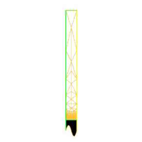
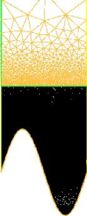
Figure 6: The microscopic periodic cell after adaptative mesh refinement

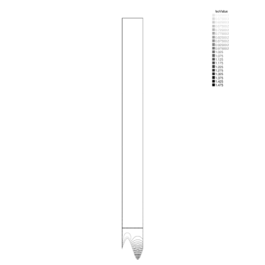
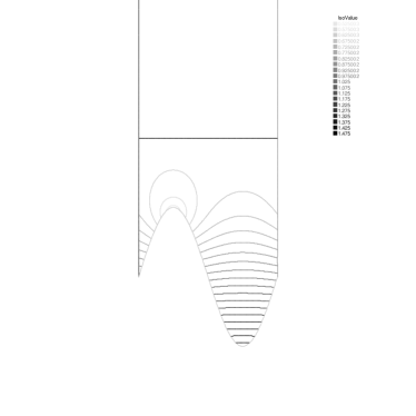
Figure 7: The microscopic periodic cell corrector $\beta^{L}$

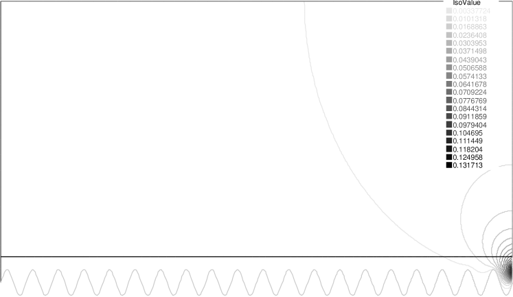
Figure 9: The microscopic corrector $\xi_{{\rm out}}^{L}$

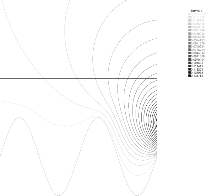
Figure 10: A zoom near the corner singularity of the microscopic corrector $\xi_{{\rm out},h}$

In figures 6 and 8, we display the meshes obtained after adaptative procedure, described below, for $\beta^{L}$ and $\xi_{{\rm out}}^{L}$. The total number of vertices used in the meshes for discretising $\beta^{L}_{h}$, $\xi_{{\rm in},h}^{L}$ and $\xi_{{\rm out},h}^{L}$ are 39000, 78000 and 79000. In the simulation of $\beta^{L}_{h}$ the horizontal top is set to $L:=10$. For $\xi_{{\rm in},h}^{L}$ and $\xi_{{\rm out},h}^{L}$ the vertical interface is set to $L:=20$. The contours of corresponding solutions $\beta^{L}_{h}$ and $\xi_{{\rm out},h}^{L}$ are displayed in figures 7, 9 and 10, whereas the normal derivative $\,\partial_{\nu}\beta^{L}_{h}\,$ and $-\,\partial_{\nu}\xi_{{\rm in},h}^{L}\,$ are shown to coincide along $\{0\}\times[-\frac{3}{4},1]$ in figure 3.

Figure 3: Normal derivatives $\,\partial_{\nu}\beta^{L}\,$ and $\,\partial_{\nu}\xi_{{\rm out}}^{L}\,$ on $E$, the vertical interface

We perform a single microscopic computation. Then we re-scale the boundary layer to the macroscopic domain setting

$$\beta^{L}_{\epsilon,h}(x):=\beta^{L}_{h}\left(\frac{x}{\epsilon}\right),\quad\xi_{{\rm in},\epsilon,h}^{L}(x):=\xi_{{\rm in},h}^{L}\left(\frac{x}{\epsilon}\right),\quad\xi_{{\rm out},\epsilon,h}^{L}(x):=\xi_{{\rm out},h}^{L}\left(\frac{x}{\epsilon}\right),\quad\forall x\in\Omega^{\epsilon}.$$

We quantify the interpolation error with respect to $\epsilon$.

$${\left\|{(\beta_{\epsilon,h}^{L}-\beta)\left(\frac{\cdot}{\epsilon}\right)}\right\|}_{L^{2}({\Omega^{0}})}\leq\sqrt{\epsilon}\left({\left\|{\beta_{h}^{L}-\beta^{L}}\right\|}_{L^{2}(Z^{+})}+{\left\|{\beta^{L}-\beta}\right\|}_{L^{2}(Z^{+})}\right)\leq k\sqrt{\epsilon}h_{m}^{s}{\left|{\beta^{L}}\right|}_{H^{s}({Z^{+}\cup\Gamma\cup P})}$$

where $s$ is a constant dependent on the boundary’s regularity, and $h_{m}$ a fixed maximum mesh size on the microscopic level, independent on $\epsilon$. In the same way one can set

$${\left\|{(\xi_{{\rm out},h}^{L}-\xi_{\rm out})\left(\frac{\cdot}{\epsilon}\right)}\right\|}_{L^{2}({\Omega^{0}})} \leq\epsilon\left({\left\|{\xi_{{\rm out},h}^{L}-\xi_{{\rm out}}^{L}}\right\|}_{L^{2}(\Pi^{L}_{-})}+{\left\|{\xi_{{\rm out}}^{L}-\xi_{\rm out}}\right\|}_{L^{2}(\Pi^{L}_{-})}\right)$$

$$\leq k\epsilon\left(h_{m}^{2}{\left\|{\xi_{{\rm out}}^{L}}\right\|}_{H^{2,\nu}(\Pi_{-}^{L})}+kL{\left\|{\xi_{{\rm out}}^{L}-\xi_{\rm out}}\right\|}_{W^{0,2}_{-1}(\Pi^{L\,\prime}_{-})}\right)\leq k\,\epsilon,$$

where $\nu$ is a real parameter depending on the angle of the corner of $\Pi_{-}$ at $(0,f(0))$, and $H^{2,\nu}$ the weighted space defined p.388 Definition 8.4.1.1 [8], that takes into account the corner singularity of second derivatives of $\xi_{{\rm out}}^{L}$. These estimates give an upper bound on the convergence rate for the full boundary layer $u^{1,\infty}_{\epsilon}$, namely:

$${\left\|{u^{\epsilon}_{h}-u^{1,\infty}_{\epsilon,h}}\right\|}_{L^{2}({\Omega^{0}})} \leq{\left\|{u^{\epsilon}_{h}-u^{\epsilon}}\right\|}_{L^{2}({\Omega^{0}})}+{\left\|{u^{\epsilon}-u^{1,\infty}_{\epsilon}}\right\|}_{L^{2}({\Omega^{0}})}+{\left\|{u^{1,\infty}_{\epsilon}-u^{1,\infty}_{\epsilon,h}}\right\|}_{L^{2}({\Omega^{0}})}$$ (18)

$$\leq H^{2}{\left\|{u^{\epsilon}}\right\|}_{H^{2,\nu}(\Omega^{\epsilon})}+k\epsilon^{\frac{3}{2}},$$

where $H$ is a macroscopic mesh size presented in the next paragraph.

Rough solutions

When computing numerical approximations of $u^{\epsilon}$, one has to play with 3 concepts that are interdependent: $h$ the mesh-size, $\epsilon$ the roughness size, and corner singularities that depend on the shape of the domain.

In the periodic case considered in [4], and for $f\in C^{\infty}(]0,1])$, in order to avoid that the roughness size goes under the mesh-size, one could discretise the solution on a mesh such that $h\leq c\,\epsilon$. Due to estimates on the interpolation error and $H^{2}(\Omega^{\epsilon})$ regularity, one obtains a good numerical agreement for convergence rates between theoretical and numerical results (see [4]).

In the non-periodic setting, corner singularities occur near $\Gamma_{\rm out}$. In order to obtain convergent numerical approximations of $u^{\epsilon}$ near $\Gamma_{\rm out}$, one should refine the mesh in the neighbourhood of $(1,\epsilon f(1/\epsilon))$. At the same time, in the regular zones, the mesh-size should stil be refined at least linearly with respect to $\epsilon$ (as in the peridic setting [4]). This complicates the local size of elements with respect to the size of the mesh ([8] p.384). Thus, simply setting uniformly $h:=c\epsilon$ does not provide accurate convergence results. On the other hand, one aims to have a strong control on the mesh size far from the corner: for instance in these zones, the mesh-size could be fixed on a uniform grid. These considerations led us to use an overlapping Schwartz algorithm [18]; we split $\Omega^{\epsilon}$ in two parts: ${\Omega^{0}}$ is discretised with a structured grid of size $H:=k\epsilon^{\gamma}$ ($\gamma$ is discussed later), whereas a second domain reads

$$\Omega^{1,\epsilon}:=\Omega^{\epsilon}\cap\left\{x\in\mathbb{R}\;\text{ s.t. }\;x_{2}<\frac{\epsilon}{10}\right\}$$

and contains the rough sub-layer. On $\Omega^{1,\epsilon}$ we perform mesh adaptation in order to capture geometrical and corner singularities. The maximum/minimum mesh-sizes are set:

$$h_{\min}=\min_{K\in{\cal T}_{K}}h_{K},\quad h_{\max}=\min_{K\in{\cal T}_{K}}h_{K}$$

where $h_{K}$ is the diameter of triangle $K$ in the triangulation ${\cal T}_{K}$ of $\Omega^{1,\epsilon}$. At each step $m$ of the Schwartz algorithm, we solve two problems. We set ${\cal U}^{m}_{\epsilon}$ to be the solution of

$$\left\{\begin{aligned} &\Delta{\cal U}^{m}_{\epsilon}=0,\text{ in }{\Omega^{0}},\\ &{\cal U}^{m}_{\epsilon}=1,\text{ on }\Gamma^{1},\\ &{\cal U}^{m}_{\epsilon}={\cal V}_{\epsilon}^{(m-1)},\text{ on }{\Gamma^{0}},\\ &\,\partial_{\nu}{\cal U}^{m}_{\epsilon}\,=0,\text{ on }\Gamma_{\rm in}^{\prime}\cup\Gamma_{\rm out}^{\prime},\end{aligned}\right.$$

and ${\cal V}^{m}_{\epsilon}$ solves

$$\left\{\begin{aligned} &\Delta{\cal V}^{m}_{\epsilon}=0,\text{ in }\Omega^{1,\epsilon},\\ &{\cal V}^{m}_{\epsilon}=0,\text{ on }{\Gamma^{\epsilon}},\\ &{\cal V}^{m}_{\epsilon}={\cal U}^{m}_{\epsilon},\text{ on }\left\{x_{2}=\frac{\epsilon}{10}\right\},\\ &\,\partial_{\nu}{\cal V}^{m}_{\epsilon}\,=0,\text{ on }({\Gamma_{\rm in}}\cup\Gamma_{\rm out})\cap\left\{x\in\mathbb{R}\;\text{ s.t. }\;x_{2}<\frac{\epsilon}{10}\right\},\end{aligned}\right.$$

and we iterate the procedure until

$$\int_{(0,1)\times\{0\}\cup(0,1)\times\{\frac{\epsilon}{10}\}}({\cal U}^{m}_{\epsilon}-{\cal V}^{m}_{\epsilon})^{2}d\sigma(x)<{\rm tol},$$

where tol is a constant set to 10^-10. During this step both meshes are kept fixed.

Then we refine the sub-layer mesh ${\cal T}_{K}$ in order to account the corner singularity. This step provides a new mesh-size distribution updating $h_{\min}$ and $h_{\max}$. We use adaptative techniques presented p. 92 of the freefem++ reference manual [10]. This procedure is compatible with the mesh requirements displayed in Theorem 8.4.1.6 p. 392 in [8] and guarantees standard interpolation errors with respect to the mesh size.

We iterate these two steps: solve the Schwartz domain decomposition problem and then adapt the mesh. The iterative algorithm stops when $h_{\max}<H$. Through this algorithm we insure both a given mesh size $H$ and a refined mesh near the corner.

We tested different values of $\gamma$ where setting $H=k\epsilon^{\gamma}$, $k$ a is given constant, choosing $\gamma\geq\frac{5}{4}$ does no more change convergence results below. We plot in fig. 4, $h_{\max}$ and $h_{\min}$ as functions of $\epsilon$. The adaptative process gives approximately $h_{\min}\sim c\epsilon^{2.29}$.

Figure 4: Mesh sizes $h_{\min}$ and $h_{\max}$ as functions of $\epsilon$

We plot in fig. 11, the meshes obtained thanks to our iterative scheme for $\epsilon\in\{{\frac{1}{2}},\frac{1}{3}\}$. In fig. 12, we display the corresponding solutions $u^{\epsilon}_{h}$. Next, we construct boundary layers using microscopic correctors above. We compute the errors $u^{\epsilon}_{h}-u^{0}$, $u^{\epsilon}_{h}-u^{1}$, $u^{\epsilon}_{h}-u^{1,\infty}_{\epsilon,\#,h}$ and $u^{\epsilon}_{h}-u^{1,\infty}_{\epsilon,h}$ in the $L^{2}({\Omega^{0}})$ norms, and display them as a function of $\epsilon$ in fig.5.

Figure 5: Errors in the $L^{2}({\Omega^{0}}_{h})$ (left) and the $H^{1}(\Omega^{\epsilon}_{h})$ (right) norms with respect to $\epsilon$

The numerical convergence rate, obtained by interpolating results above as a powers of $\epsilon$, is displayed in table 1.

norm / approx.	$u^{\epsilon}_{h}-u^{0}$	$u^{\epsilon}_{h}-u^{1}$	$u^{\epsilon}_{h}-u^{1,\infty}_{\epsilon,\#,h}$	$u^{\epsilon}_{h}-u^{1,\infty}_{\epsilon,h}$
$L^{2}({\Omega^{0}})$	0.78783	1.11	1.1	1.462
$H^{1}({\Omega^{0}})$	0.787	0.6869	0.70	1.346347

Table 1: The errors convergence rates displayed as powers of $\epsilon$

Discussion

When the vertical correctors are not present, the boundary layer approximation is not only less accurate but also the rate of convergence is less than first order, the difference is visible in $L^{2}({\Omega^{0}})$ but is significant in the $H^{1}({\Omega^{0}})$ norm. Nevertheless, and as explained above, when using a single microscopic computation of the correctors for every $\epsilon$, it is not possible to get better convergence results than $\epsilon^{\frac{3}{2}}$. This is actually what we obtain for our more accurate approximation $u^{1,\infty}_{\epsilon,h}$. This validates our theoretical results. The surprising phenomenon that we are at this point not able to justify is the poor convergence rate of the wall law $u^{1}$, that should according to our estimates be $\epsilon^{\frac{3}{2}}$. Observed in [4], $u^{1}$ performs even worse convergence rate than $u^{0}$ in the $H^{1}({\Omega^{0}})$ norm. The results of Theorem 2.2 are fairly approximated for what concerns the $H^{1}({\Omega^{0}})$ error of $u^{1,\infty}_{\epsilon,h}$.

7 Conclusion

Our approach provides an almost complete understanding of the non-periodic case for lateral homogeneous Neumann boundary conditions in the straight case, (no curvature effects of the rough boundary [17]). A forthcoming paper should adapt these results to the case mentioned in the introduction: a smooth boundary forward and backward the rough domain via domain decomposition techniques. Another extension to the Stokes system should follow as well.

Acknowledgements.

The author would like to thank C. Amrouche for his advises and support, S. Nazarov for fruitful discussions and clarifications, and H. Teismann for proof reading. This research was partially funded by Cardiatis, an industrial partner designing and commercializing metallic wired stents.

Figure 8: The microscopic domain of $\xi_{{\rm out}}^{L}$ after adaptative mesh refinement

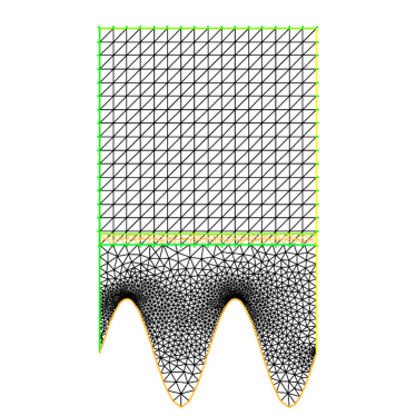
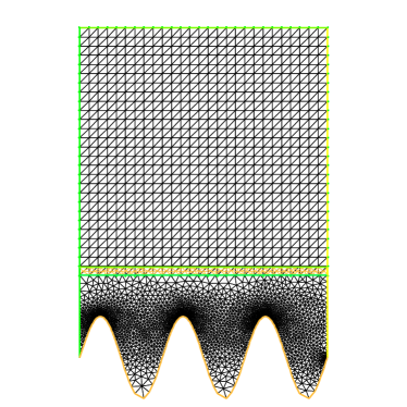
Figure 11: The meshes for the rough solution for $\epsilon\in\{{\frac{1}{2}},{1}/{3}\}$ using a decomposition method

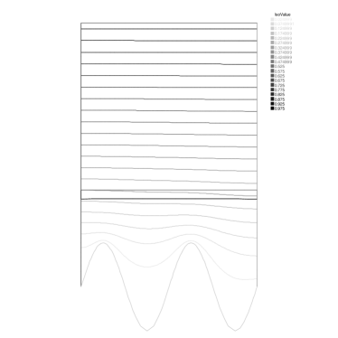
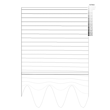
Figure 12: The rough solution computed for $\epsilon\in\{{\frac{1}{2}},{1}/{3}\}$ using a decomposition method

References

• [1] C. Amrouche, V. Girault, and J. Giroire. Weighted sobolev spaces and laplace’s equation in $\mathbb{R}^{n}$. Journal des Mathematiques Pures et Appliquees, 73:579–606, January 1994.
• [2] C. Amrouche, V. Girault, and J. Giroire. Dirichlet and neumann exterior problems for the n-dimensional laplace operator an approach in weighted sobolev spaces. Journal des Mathematiques Pures et Appliquees, 76:55–81(27), January 1997.
• [3] E. Bonnetier, D. Bresch, and V. Milisic. Blood flow modelling in stented arteries: new convergence results of first order boundary layers and wall-laws for a rough neumann-laplace problem. submitted.
• [4] D. Bresch and V. Milisic. High order multi-scale wall laws : part i, the periodic case. accepted for publication in Quart. Appl. Math. 2008.
• [5] D. Bresch and V. Milisic. Towards implicit multi-scale wall laws. accepted for publication in C. R. Acad. Sciences, Série Mathématiques, 2008.
• [6] L. C. Evans. Partial differential equations, volume 19 of Graduate Studies in Mathematics. American Mathematical Society, Providence, RI, 1998.
• [7] D. Gilbarg and N. S. Trudinger. Elliptic partial differential equations of second order. Classics in Mathematics. Springer-Verlag, Berlin, 2001. Reprint of the 1998 edition.
• [8] P. Grisvard. Elliptic problems in nonsmooth domains, volume 24 of Monographs and Studies in Mathematics. Pitman (Advanced Publishing Program), Boston, MA, 1985.
• [9] B. Hanouzet. Espaces de Sobolev avec poids application au problème de Dirichlet dans un demi espace. Rend. Sem. Mat. Univ. Padova, 46:227–272, 1971.
• [10] F. Hecht, O. Pironneau, A. Le Hyaric, and Ohtsuka K. Freefem++. Laboratoire Jacques-Louis Lions, Universite Pierre et Marie Curie, Paris, 2005.
• [11] W. Jäger and A. Mikelić. On the interface boundary condition of Beavers, Joseph, and Saffman. SIAM J. Appl. Math., 60(4):1111–1127, 2000.
• [12] W. Jäger and A. Mikelić. On the roughness-induced effective boundary condition for an incompressible viscous flow. J. Diff. Equa., 170:96–122, 2001.
• [13] W. Jäger, A. Mikelić, and N. Neuss. Asymptotic analysis of the laminar viscous flow over a porous bed. SIAM J. Sci. Comput., 22(6):2006–2028, 2001.
• [14] Willi Jäger and Andro Mikelić. On the boundary conditions at the contact interface between a porous medium and a free fluid. Ann. Scuola Norm. Sup. Pisa Cl. Sci. (4), 23(3):403–465, 1996.
• [15] A. Kufner. Weighted Sobolev spaces. BSB B. G. Teubner Verlagsgesellschaft, teubner-texte zur mathematik edition, 1980.
• [16] J. Nečas. Les méthodes directes en théorie des équations elliptiques. Masson et Cie, Éditeurs, Paris, 1967.
• [17] N. Neuss, M. Neuss-Radu, and A. Mikelić. Effective laws for the poisson equation on domains with curved oscillating boundaries. Applicable Analysis, 85:479–502, 2006.
• [18] A. Quarteroni and A. Valli. Domain decomposition methods for partial differential equations. Numerical Mathematics and Scientific Computation. Oxford Science Publication, Oxford, 1999.
• [19] E. Sanchez-Palencia and A. Zaoui. Homogenization techniques for composite media, volume 272 of Lecture Notes in Physics. Springer-Verlag., 1987.
Refer to caption
Refer to caption