NRCPS-HE-56-08
December, 2008
Production of charged spin-two gauge bosons
Spyros Konitopoulos
and
George Savvidy
Institute of Nuclear Physics,
Demokritos National Research Center
We are considering the production of charged spin-two gauge bosons in the gluon-gluon
scattering and calculating polarized cross sections for each set of helicity
orientations of initial and final particles.
The angular dependence of this cross section is being compared with
the gluon-gluon scattering cross section in QCD .
1 Introduction
An infinite tower of massive particles of high spin naturally
appears in the spectrum of different string field theories.
It is generally expected that in the tensionless limit
or, what is equivalent, at high energy and fixed angle scattering
the string spectrum becomes effectively massless
[1 , 2 , 3 , 4 , 5 , 6 ] . In the open string theory with Chan-Paton charges these
massless states can combine into the infinite tower
of non-Abelian tensor gauge fields [7 ] and one could guess that the
corresponding Lagrangian quantum field theory should be described
by some kind of extension of the Yang-Mills theory.
A possible extension of Yang-Mills theory which includes non-Abelian tensor gauge fileds
was suggested recently in [10 , 11 , 12 ] .
The non-Abelian gauge fields are defined as rank-(s+1) tensor gauge fields
A μ λ 1 … λ s a subscript superscript 𝐴 𝑎 𝜇 subscript 𝜆 1 … subscript 𝜆 𝑠 A^{a}_{\mu\lambda_{1}...\lambda_{s}} [10 , 11 , 12 ]
ℒ = ℒ 1 + ℒ 2 + g 3 ℒ 3 … . , ℒ subscript ℒ 1 subscript ℒ 2 subscript 𝑔 3 subscript ℒ 3 … {\cal L}~{}=~{}{{\cal L}}_{1}+{{\cal L}}_{2}+g_{3}{{\cal L}}_{3}...., (1)
where ℒ 1 subscript ℒ 1 {{\cal L}}_{1} ℒ s ( s = 2 , 3 , . . ) {{\cal L}}_{s}~{}(s=2,3,..) extended gauge transformations
[10 , 11 , 12 ] .
The Lagrangian ℒ ℒ {\cal L} [10 , 11 , 12 ] :
ℒ 1 = subscript ℒ 1 absent \displaystyle{{\cal L}}_{1}= − \displaystyle- 1 4 G μ ν a G μ ν a , 1 4 subscript superscript 𝐺 𝑎 𝜇 𝜈 subscript superscript 𝐺 𝑎 𝜇 𝜈 \displaystyle{1\over 4}G^{a}_{\mu\nu}G^{a}_{\mu\nu},
ℒ 2 = subscript ℒ 2 absent \displaystyle{{\cal L}}_{2}= − \displaystyle- 1 4 G μ ν , λ a G μ ν , λ a − 1 4 G μ ν a G μ ν , λ λ a + 1 4 subscript superscript 𝐺 𝑎 𝜇 𝜈 𝜆
subscript superscript 𝐺 𝑎 𝜇 𝜈 𝜆
limit-from 1 4 subscript superscript 𝐺 𝑎 𝜇 𝜈 subscript superscript 𝐺 𝑎 𝜇 𝜈 𝜆 𝜆
\displaystyle{1\over 4}G^{a}_{\mu\nu,\lambda}G^{a}_{\mu\nu,\lambda}-{1\over 4}G^{a}_{\mu\nu}G^{a}_{\mu\nu,\lambda\lambda}+
+ \displaystyle+ 1 4 G μ ν , λ a G μ λ , ν a + 1 4 G μ ν , ν a G μ λ , λ a + 1 2 G μ ν a G μ λ , ν λ a , 1 4 subscript superscript 𝐺 𝑎 𝜇 𝜈 𝜆
subscript superscript 𝐺 𝑎 𝜇 𝜆 𝜈
1 4 subscript superscript 𝐺 𝑎 𝜇 𝜈 𝜈
subscript superscript 𝐺 𝑎 𝜇 𝜆 𝜆
1 2 subscript superscript 𝐺 𝑎 𝜇 𝜈 subscript superscript 𝐺 𝑎 𝜇 𝜆 𝜈 𝜆
\displaystyle{1\over 4}G^{a}_{\mu\nu,\lambda}G^{a}_{\mu\lambda,\nu}+{1\over 4}G^{a}_{\mu\nu,\nu}G^{a}_{\mu\lambda,\lambda}+{1\over 2}G^{a}_{\mu\nu}G^{a}_{\mu\lambda,\nu\lambda},
where the generalized field strength tensors are:
G μ ν a subscript superscript 𝐺 𝑎 𝜇 𝜈 \displaystyle G^{a}_{\mu\nu} = \displaystyle= ∂ μ A ν a − ∂ ν A μ a + g f a b c A μ b A ν c , subscript 𝜇 subscript superscript 𝐴 𝑎 𝜈 subscript 𝜈 subscript superscript 𝐴 𝑎 𝜇 𝑔 superscript 𝑓 𝑎 𝑏 𝑐 subscript superscript 𝐴 𝑏 𝜇 subscript superscript 𝐴 𝑐 𝜈 \displaystyle\partial_{\mu}A^{a}_{\nu}-\partial_{\nu}A^{a}_{\mu}+gf^{abc}~{}A^{b}_{\mu}~{}A^{c}_{\nu},
G μ ν , λ a subscript superscript 𝐺 𝑎 𝜇 𝜈 𝜆
\displaystyle G^{a}_{\mu\nu,\lambda} = \displaystyle= ∂ μ A ν λ a − ∂ ν A μ λ a + g f a b c ( A μ b A ν λ c + A μ λ b A ν c ) , subscript 𝜇 subscript superscript 𝐴 𝑎 𝜈 𝜆 subscript 𝜈 subscript superscript 𝐴 𝑎 𝜇 𝜆 𝑔 superscript 𝑓 𝑎 𝑏 𝑐 subscript superscript 𝐴 𝑏 𝜇 subscript superscript 𝐴 𝑐 𝜈 𝜆 subscript superscript 𝐴 𝑏 𝜇 𝜆 subscript superscript 𝐴 𝑐 𝜈 \displaystyle\partial_{\mu}A^{a}_{\nu\lambda}-\partial_{\nu}A^{a}_{\mu\lambda}+gf^{abc}(~{}A^{b}_{\mu}~{}A^{c}_{\nu\lambda}+A^{b}_{\mu\lambda}~{}A^{c}_{\nu}~{}), (3)
G μ ν , λ ρ a subscript superscript 𝐺 𝑎 𝜇 𝜈 𝜆 𝜌
\displaystyle G^{a}_{\mu\nu,\lambda\rho} = \displaystyle= ∂ μ A ν λ ρ a − ∂ ν A μ λ ρ a + g f a b c ( A μ b A ν λ ρ c + A μ λ b A ν ρ c + A μ ρ b A ν λ c + A μ λ ρ b A ν c ) . subscript 𝜇 subscript superscript 𝐴 𝑎 𝜈 𝜆 𝜌 subscript 𝜈 subscript superscript 𝐴 𝑎 𝜇 𝜆 𝜌 𝑔 superscript 𝑓 𝑎 𝑏 𝑐 subscript superscript 𝐴 𝑏 𝜇 subscript superscript 𝐴 𝑐 𝜈 𝜆 𝜌 subscript superscript 𝐴 𝑏 𝜇 𝜆 subscript superscript 𝐴 𝑐 𝜈 𝜌 subscript superscript 𝐴 𝑏 𝜇 𝜌 subscript superscript 𝐴 𝑐 𝜈 𝜆 subscript superscript 𝐴 𝑏 𝜇 𝜆 𝜌 subscript superscript 𝐴 𝑐 𝜈 \displaystyle\partial_{\mu}A^{a}_{\nu\lambda\rho}-\partial_{\nu}A^{a}_{\mu\lambda\rho}+gf^{abc}(~{}A^{b}_{\mu}~{}A^{c}_{\nu\lambda\rho}+A^{b}_{\mu\lambda}~{}A^{c}_{\nu\rho}+A^{b}_{\mu\rho}~{}A^{c}_{\nu\lambda}+A^{b}_{\mu\lambda\rho}~{}A^{c}_{\nu}~{}).
The definition of
the Lagrangian forms ℒ s subscript ℒ 𝑠 {{\cal L}}_{s} [10 , 11 , 12 ] .
The above expressions define interacting gauge field theory with infinite
many gauge fields. Not much is known about physical properties of such gauge
field theories and in the present paper we shall focus our attention on the lower-rank
tensor gauge field A μ λ a subscript superscript 𝐴 𝑎 𝜇 𝜆 A^{a}_{\mu\lambda}
Our intention in this article is to calculate the leading-order differential
cross section of spin-two tensor gauge boson production by a pair of vector
gauge bosons in the process V + V → T + T → 𝑉 𝑉 𝑇 𝑇 V+V\rightarrow T+T 4 5 8
Below we shall present the Feynman diagrams for the given process,
the expressions for the corresponding vertices and transition amplitudes.
Then we shall calculate the polarized cross sections for each set of helicity orientations of the initial
and final particles (see formulas
(33 34 35 37 V + V → V + V → 𝑉 𝑉 𝑉 𝑉 V+V\rightarrow V+V 46 47 48 38 V + V → V + V → 𝑉 𝑉 𝑉 𝑉 V+V\rightarrow V+V [9 ] and in Appendix B
we shall demonstrate the gauge invariance of the transition amplitude.
2 Summary of Feynman rules
The Feynman rules for the Lagrangian (1 A α a , A α α ′ a , … subscript superscript 𝐴 𝑎 𝛼 subscript superscript 𝐴 𝑎 𝛼 superscript 𝛼 ′ …
A^{a}_{\alpha},~{}A^{a}_{\alpha\alpha^{\prime}},... [10 , 11 , 12 ] .
The indices of the symmetry group G are a , b = 1 , … , d ( G ) formulae-sequence 𝑎 𝑏
1 … 𝑑 𝐺
a,b=1,...,d(G) d ( G ) 𝑑 𝐺 d(G)
D a b α β ( k ) = − i k 2 η α β δ a b . subscript superscript 𝐷 𝛼 𝛽 𝑎 𝑏 𝑘 𝑖 superscript 𝑘 2 superscript 𝜂 𝛼 𝛽 subscript 𝛿 𝑎 𝑏 \displaystyle D^{\alpha\beta}_{ab}(k)=-{i\over k^{2}}\eta^{\alpha\beta}\delta_{ab}. (4)
The second-rank tensor gauge field A α α ´ subscript 𝐴 𝛼 ´ 𝛼 A_{\alpha\acute{\alpha}} [10 , 11 , 12 ] .
The kinetic operator of the tensor gauge bosons
H α α ´ γ γ ´ ( k ) subscript 𝐻 𝛼 ´ 𝛼 𝛾 ´ 𝛾 𝑘 \displaystyle H_{\alpha\acute{\alpha}\gamma\acute{\gamma}}(k) = \displaystyle= ( − η α γ η α ´ γ ´ + 1 2 η α γ ´ η α ´ γ + 1 2 η α α ´ η γ γ ´ ) k 2 + η α γ k α ´ k γ ´ + η α ´ γ ´ k α k γ subscript 𝜂 𝛼 𝛾 subscript 𝜂 ´ 𝛼 ´ 𝛾 1 2 subscript 𝜂 𝛼 ´ 𝛾 subscript 𝜂 ´ 𝛼 𝛾 1 2 subscript 𝜂 𝛼 ´ 𝛼 subscript 𝜂 𝛾 ´ 𝛾 superscript 𝑘 2 subscript 𝜂 𝛼 𝛾 subscript 𝑘 ´ 𝛼 subscript 𝑘 ´ 𝛾 subscript 𝜂 ´ 𝛼 ´ 𝛾 subscript 𝑘 𝛼 subscript 𝑘 𝛾 \displaystyle(-\eta_{\alpha\gamma}\eta_{\acute{\alpha}\acute{\gamma}}+{1\over 2}\eta_{\alpha\acute{\gamma}}\eta_{\acute{\alpha}\gamma}+{1\over 2}\eta_{\alpha\acute{\alpha}}\eta_{\gamma\acute{\gamma}})k^{2}+\eta_{\alpha\gamma}k_{\acute{\alpha}}k_{\acute{\gamma}}+\eta_{\acute{\alpha}\acute{\gamma}}k_{\alpha}k_{\gamma} (5)
− \displaystyle- 1 2 ( η α γ ´ k α ´ k γ + η α ´ γ k α k γ ´ + η α α ´ k γ k γ ´ + η γ γ ´ k α k α ´ ) 1 2 subscript 𝜂 𝛼 ´ 𝛾 subscript 𝑘 ´ 𝛼 subscript 𝑘 𝛾 subscript 𝜂 ´ 𝛼 𝛾 subscript 𝑘 𝛼 subscript 𝑘 ´ 𝛾 subscript 𝜂 𝛼 ´ 𝛼 subscript 𝑘 𝛾 subscript 𝑘 ´ 𝛾 subscript 𝜂 𝛾 ´ 𝛾 subscript 𝑘 𝛼 subscript 𝑘 ´ 𝛼 \displaystyle{1\over 2}(\eta_{\alpha\acute{\gamma}}k_{\acute{\alpha}}k_{\gamma}+\eta_{\acute{\alpha}\gamma}k_{\alpha}k_{\acute{\gamma}}+\eta_{\alpha\acute{\alpha}}k_{\gamma}k_{\acute{\gamma}}+\eta_{\gamma\acute{\gamma}}k_{\alpha}k_{\acute{\alpha}})
is a gauge invariant operator
k α H α α ´ γ γ ´ = 0 , k α ´ H α α ´ γ γ ´ = 0 . formulae-sequence subscript 𝑘 𝛼 subscript 𝐻 𝛼 ´ 𝛼 𝛾 ´ 𝛾 0 subscript 𝑘 ´ 𝛼 subscript 𝐻 𝛼 ´ 𝛼 𝛾 ´ 𝛾 0 k_{\alpha}H_{\alpha\acute{\alpha}\gamma\acute{\gamma}}=0,~{}k_{\acute{\alpha}}H_{\alpha\acute{\alpha}\gamma\acute{\gamma}}=0. H α α ´ γ γ ´ ( k ) f γ γ ´ ( k ) = 0 subscript 𝐻 𝛼 ´ 𝛼 𝛾 ´ 𝛾 𝑘 superscript 𝑓 𝛾 ´ 𝛾 𝑘 0 H_{\alpha\acute{\alpha}\gamma\acute{\gamma}}(k)f^{\gamma\acute{\gamma}}(k)=0 Δ α α ′ β β ′ a b ( k ) subscript superscript Δ 𝑎 𝑏 𝛼 superscript 𝛼 ′ 𝛽 superscript 𝛽 ′ 𝑘 \Delta^{ab}_{\alpha\alpha^{\prime}\beta\beta^{\prime}}(k) H α α ´ γ γ ´ f i x ( k ) Δ λ λ ´ γ γ ´ ( k ) = i η α λ η α ´ λ ´ subscript superscript 𝐻 𝑓 𝑖 𝑥 𝛼 ´ 𝛼 𝛾 ´ 𝛾 𝑘 subscript superscript Δ 𝛾 ´ 𝛾 𝜆 ´ 𝜆 𝑘 𝑖 subscript 𝜂 𝛼 𝜆 subscript 𝜂 ´ 𝛼 ´ 𝜆 H^{fix}_{\alpha\acute{\alpha}\gamma\acute{\gamma}}(k)\Delta^{\gamma\acute{\gamma}}_{~{}~{}~{}\lambda\acute{\lambda}}(k)=i\eta_{\alpha\lambda}\eta_{\acute{\alpha}\acute{\lambda}}~{}~{}
Δ α α ′ β β ′ a b ( k ) = − i k 2 Π α α ′ β β ′ δ a b , subscript superscript Δ 𝑎 𝑏 𝛼 superscript 𝛼 ′ 𝛽 superscript 𝛽 ′ 𝑘 𝑖 superscript 𝑘 2 subscript Π 𝛼 superscript 𝛼 ′ 𝛽 superscript 𝛽 ′ superscript 𝛿 𝑎 𝑏 \Delta^{ab}_{\alpha\alpha^{\prime}\beta\beta^{\prime}}(k)=-{i\over k^{2}}~{}\Pi_{\alpha\alpha^{\prime}\beta\beta^{\prime}}~{}\delta^{ab}, (6)
where the residue can be represented as a sum of λ = ± 2 𝜆 plus-or-minus 2 \lambda=\pm 2 λ = 0 𝜆 0 \lambda=0
Π α α ′ β β ′ = ( η α β η α ′ β ′ + η α β ′ η α ′ β − η α α ′ η β β ′ ) + 1 3 ( η α β η α ′ β ′ − η α β ′ η α ′ β ) . subscript Π 𝛼 superscript 𝛼 ′ 𝛽 superscript 𝛽 ′ subscript 𝜂 𝛼 𝛽 subscript 𝜂 superscript 𝛼 ′ superscript 𝛽 ′ subscript 𝜂 𝛼 superscript 𝛽 ′ subscript 𝜂 superscript 𝛼 ′ 𝛽 subscript 𝜂 𝛼 superscript 𝛼 ′ subscript 𝜂 𝛽 superscript 𝛽 ′ 1 3 subscript 𝜂 𝛼 𝛽 subscript 𝜂 superscript 𝛼 ′ superscript 𝛽 ′ subscript 𝜂 𝛼 superscript 𝛽 ′ subscript 𝜂 superscript 𝛼 ′ 𝛽 \displaystyle\Pi_{\alpha\alpha^{\prime}\beta\beta^{\prime}}=(\eta_{\alpha\beta}\eta_{\alpha^{\prime}\beta^{\prime}}+\eta_{\alpha\beta^{\prime}}\eta_{\alpha^{\prime}\beta}-\eta_{\alpha\alpha^{\prime}}\eta_{\beta\beta^{\prime}})+{1\over 3}(\eta_{\alpha\beta}\eta_{\alpha^{\prime}\beta^{\prime}}-\eta_{\alpha\beta^{\prime}}\eta_{\alpha^{\prime}\beta}). (7)
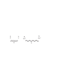
Figure 1: The vector - D μ ν a b ( k ) subscript superscript 𝐷 𝑎 𝑏 𝜇 𝜈 𝑘 D^{ab}_{\mu\nu}(k) Δ γ γ ′ λ λ ′ a b ( k ) subscript superscript Δ 𝑎 𝑏 𝛾 superscript 𝛾 ′ 𝜆 superscript 𝜆 ′ 𝑘 \Delta^{ab}_{\gamma\gamma^{{}^{\prime}}\lambda\lambda^{{}^{\prime}}}(k)
The standard Yang-Mills three-vector boson interaction vertex
VVV in the momentum representation has the form
𝒱 α β γ a b c ( k , p , q ) = − g f a b c F α β γ ( k , p , q ) = − g f a b c [ η α β ( p − k ) γ + η α γ ( k − q ) β + η β γ ( q − p ) α ] . subscript superscript 𝒱 𝑎 𝑏 𝑐 𝛼 𝛽 𝛾 𝑘 𝑝 𝑞 𝑔 superscript 𝑓 𝑎 𝑏 𝑐 subscript 𝐹 𝛼 𝛽 𝛾 𝑘 𝑝 𝑞 𝑔 superscript 𝑓 𝑎 𝑏 𝑐 delimited-[] subscript 𝜂 𝛼 𝛽 subscript 𝑝 𝑘 𝛾 subscript 𝜂 𝛼 𝛾 subscript 𝑘 𝑞 𝛽 subscript 𝜂 𝛽 𝛾 subscript 𝑞 𝑝 𝛼 {{\cal V}}^{abc}_{\alpha\beta\gamma}(k,p,q)=-gf^{abc}F_{\alpha\beta\gamma}(k,p,q)=-gf^{abc}[\eta_{\alpha\beta}(p-k)_{\gamma}+\eta_{\alpha\gamma}(k-q)_{\beta}+\eta_{\beta\gamma}(q-p)_{\alpha}]. (8)
The interaction vertex of vector gauge boson V with two
tensor gauge bosons T - the VTT vertex - has the form
[11 , 12 ]
𝒱 α α ´ β γ γ ´ a b c ( k , p , q ) = − g f a b c F α α ´ β γ γ ´ , subscript superscript 𝒱 𝑎 𝑏 𝑐 𝛼 ´ 𝛼 𝛽 𝛾 ´ 𝛾 𝑘 𝑝 𝑞 𝑔 superscript 𝑓 𝑎 𝑏 𝑐 subscript 𝐹 𝛼 ´ 𝛼 𝛽 𝛾 ´ 𝛾 {\cal V}^{abc}_{\alpha\acute{\alpha}\beta\gamma\acute{\gamma}}(k,p,q)=-g~{}f^{abc}F_{\alpha\acute{\alpha}\beta\gamma\acute{\gamma}}, (9)
where
F α α ´ β γ γ ´ ( k , p , q ) subscript 𝐹 𝛼 ´ 𝛼 𝛽 𝛾 ´ 𝛾 𝑘 𝑝 𝑞 \displaystyle F_{\alpha\acute{\alpha}\beta\gamma\acute{\gamma}}(k,p,q) = \displaystyle= [ η α β ( p − k ) γ + η α γ ( k − q ) β + η β γ ( q − p ) α ] η α ´ γ ´ − limit-from delimited-[] subscript 𝜂 𝛼 𝛽 subscript 𝑝 𝑘 𝛾 subscript 𝜂 𝛼 𝛾 subscript 𝑘 𝑞 𝛽 subscript 𝜂 𝛽 𝛾 subscript 𝑞 𝑝 𝛼 subscript 𝜂 ´ 𝛼 ´ 𝛾 \displaystyle[\eta_{\alpha\beta}(p-k)_{\gamma}+\eta_{\alpha\gamma}(k-q)_{\beta}+\eta_{\beta\gamma}(q-p)_{\alpha}]\eta_{\acute{\alpha}\acute{\gamma}}-
− \displaystyle- 1 2 [ ( p − k ) γ ( η α γ ´ η α ´ β + η α α ´ η β γ ´ ) + ( k − q ) β ( η α γ ´ η α ´ γ + η α α ´ η γ γ ´ ) \displaystyle{1\over 2}[~{}(p-k)_{\gamma}(\eta_{\alpha\acute{\gamma}}\eta_{\acute{\alpha}\beta}+\eta_{\alpha\acute{\alpha}}\eta_{\beta\acute{\gamma}})+(k-q)_{\beta}(\eta_{\alpha\acute{\gamma}}\eta_{\acute{\alpha}\gamma}+\eta_{\alpha\acute{\alpha}}\eta_{\gamma\acute{\gamma}})
+ \displaystyle+ ( q − p ) α ( η α ´ γ η β γ ´ + η α ´ β η γ γ ´ ) + ( p − k ) α ´ η α β η γ γ ´ + ( p − k ) γ ´ η α β η α ´ γ subscript 𝑞 𝑝 𝛼 subscript 𝜂 ´ 𝛼 𝛾 subscript 𝜂 𝛽 ´ 𝛾 subscript 𝜂 ´ 𝛼 𝛽 subscript 𝜂 𝛾 ´ 𝛾 subscript 𝑝 𝑘 ´ 𝛼 subscript 𝜂 𝛼 𝛽 subscript 𝜂 𝛾 ´ 𝛾 subscript 𝑝 𝑘 ´ 𝛾 subscript 𝜂 𝛼 𝛽 subscript 𝜂 ´ 𝛼 𝛾 \displaystyle(q-p)_{\alpha}(\eta_{\acute{\alpha}\gamma}\eta_{\beta\acute{\gamma}}+\eta_{\acute{\alpha}\beta}\eta_{\gamma\acute{\gamma}})+(p-k)_{\acute{\alpha}}\eta_{\alpha\beta}\eta_{\gamma\acute{\gamma}}+(p-k)_{\acute{\gamma}}\eta_{\alpha\beta}\eta_{\acute{\alpha}\gamma}
+ \displaystyle+ ( k − q ) α ´ η α γ η β γ ´ + ( k − q ) γ ´ η α γ η α ´ β + ( q − p ) α ´ η β γ η α γ ´ + ( q − p ) γ ´ η α α ´ η β γ ] . \displaystyle(k-q)_{\acute{\alpha}}\eta_{\alpha\gamma}\eta_{\beta\acute{\gamma}}+(k-q)_{\acute{\gamma}}\eta_{\alpha\gamma}\eta_{\acute{\alpha}\beta}+(q-p)_{\acute{\alpha}}\eta_{\beta\gamma}\eta_{\alpha\acute{\gamma}}+(q-p)_{\acute{\gamma}}\eta_{\alpha\acute{\alpha}}\eta_{\beta\gamma}].
The Lorentz indices α α ´ 𝛼 ´ 𝛼 \alpha\acute{\alpha} k 𝑘 k γ γ ´ 𝛾 ´ 𝛾 \gamma\acute{\gamma} q 𝑞 q β 𝛽 \beta p 𝑝 p 2
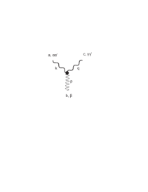
Figure 2: The interaction vertex for vector gauge boson V and
two tensor gauge bosons T
the VTT vertex - 𝒱 α α ´ β γ γ ´ a b c ( k , p , q ) subscript superscript 𝒱 𝑎 𝑏 𝑐 𝛼 ´ 𝛼 𝛽 𝛾 ´ 𝛾 𝑘 𝑝 𝑞 {\cal V}^{abc}_{\alpha\acute{\alpha}\beta\gamma\acute{\gamma}}(k,p,q) [12 ] .
Vector gauge bosons are conventionally drawn
as thin wave lines, tensor gauge bosons are thick wave lines.
The Lorentz indices α α ´ 𝛼 ´ 𝛼 \alpha\acute{\alpha} k 𝑘 k γ γ ´ 𝛾 ´ 𝛾 \gamma\acute{\gamma} q 𝑞 q β 𝛽 \beta p 𝑝 p
In the Lagrangian
(1
𝒱 α β γ δ a b c d ( k , p , q , r ) = − i g 2 f l a c f l b d ( η α β η γ δ − η α δ η β γ ) subscript superscript 𝒱 𝑎 𝑏 𝑐 𝑑 𝛼 𝛽 𝛾 𝛿 𝑘 𝑝 𝑞 𝑟 𝑖 superscript 𝑔 2 superscript 𝑓 𝑙 𝑎 𝑐 superscript 𝑓 𝑙 𝑏 𝑑 subscript 𝜂 𝛼 𝛽 subscript 𝜂 𝛾 𝛿 subscript 𝜂 𝛼 𝛿 subscript 𝜂 𝛽 𝛾 \displaystyle{{\cal V}}^{abcd}_{\alpha\beta\gamma\delta}(k,p,q,r)=-ig^{2}f^{lac}f^{lbd}(\eta_{\alpha\beta}\eta_{\gamma\delta}-\eta_{\alpha\delta}\eta_{\beta\gamma})
− i g 2 f l a d f l b c ( η α β η γ δ − η α γ η β δ ) 𝑖 superscript 𝑔 2 superscript 𝑓 𝑙 𝑎 𝑑 superscript 𝑓 𝑙 𝑏 𝑐 subscript 𝜂 𝛼 𝛽 subscript 𝜂 𝛾 𝛿 subscript 𝜂 𝛼 𝛾 subscript 𝜂 𝛽 𝛿 \displaystyle-ig^{2}f^{lad}f^{lbc}(\eta_{\alpha\beta}\eta_{\gamma\delta}-\eta_{\alpha\gamma}\eta_{\beta\delta})
− i g 2 f l a b f l c d ( η α γ η β δ − η α δ η β γ ) 𝑖 superscript 𝑔 2 superscript 𝑓 𝑙 𝑎 𝑏 superscript 𝑓 𝑙 𝑐 𝑑 subscript 𝜂 𝛼 𝛾 subscript 𝜂 𝛽 𝛿 subscript 𝜂 𝛼 𝛿 subscript 𝜂 𝛽 𝛾 \displaystyle-ig^{2}f^{lab}f^{lcd}(\eta_{\alpha\gamma}\eta_{\beta\delta}-\eta_{\alpha\delta}\eta_{\beta\gamma}) (11)
and a new interaction of two vector and two tensor gauge bosons - the VVTT vertex,
𝒱 α β γ γ ´ δ δ ´ a b c d ( k , p , q , r ) = subscript superscript 𝒱 𝑎 𝑏 𝑐 𝑑 𝛼 𝛽 𝛾 ´ 𝛾 𝛿 ´ 𝛿 𝑘 𝑝 𝑞 𝑟 absent \displaystyle{{\cal V}}^{abcd}_{\alpha\beta\gamma\acute{\gamma}\delta\acute{\delta}}(k,p,q,r)= − \displaystyle- i g 2 f l a c f l b d ( η α β η γ δ − η α δ η β γ ) η γ ´ δ ´ 𝑖 superscript 𝑔 2 superscript 𝑓 𝑙 𝑎 𝑐 superscript 𝑓 𝑙 𝑏 𝑑 subscript 𝜂 𝛼 𝛽 subscript 𝜂 𝛾 𝛿 subscript 𝜂 𝛼 𝛿 subscript 𝜂 𝛽 𝛾 subscript 𝜂 ´ 𝛾 ´ 𝛿 \displaystyle ig^{2}~{}f^{lac}f^{lbd}(\eta_{\alpha\beta}\eta_{\gamma\delta}-\eta_{\alpha\delta}\eta_{\beta\gamma})\eta_{\acute{\gamma}\acute{\delta}}
− \displaystyle- i g 2 f l a d f l b c ( η α β η γ δ − η α γ η β δ ) η γ ´ δ ´ 𝑖 superscript 𝑔 2 superscript 𝑓 𝑙 𝑎 𝑑 superscript 𝑓 𝑙 𝑏 𝑐 subscript 𝜂 𝛼 𝛽 subscript 𝜂 𝛾 𝛿 subscript 𝜂 𝛼 𝛾 subscript 𝜂 𝛽 𝛿 subscript 𝜂 ´ 𝛾 ´ 𝛿 \displaystyle ig^{2}~{}f^{lad}f^{lbc}(\eta_{\alpha\beta}\eta_{\gamma\delta}-\eta_{\alpha\gamma}\eta_{\beta\delta})\eta_{\acute{\gamma}\acute{\delta}}
− \displaystyle- i g 2 f l a b f l c d ( η α γ η β δ − η α δ η β γ ) η γ ´ δ ´ 𝑖 superscript 𝑔 2 superscript 𝑓 𝑙 𝑎 𝑏 superscript 𝑓 𝑙 𝑐 𝑑 subscript 𝜂 𝛼 𝛾 subscript 𝜂 𝛽 𝛿 subscript 𝜂 𝛼 𝛿 subscript 𝜂 𝛽 𝛾 subscript 𝜂 ´ 𝛾 ´ 𝛿 \displaystyle ig^{2}~{}f^{lab}f^{lcd}(\eta_{\alpha\gamma}\eta_{\beta\delta}-\eta_{\alpha\delta}\eta_{\beta\gamma})\eta_{\acute{\gamma}\acute{\delta}}
+ i 2 g 2 f l a c f l b d [ \displaystyle+{i\over 2}g^{2}~{}f^{lac}f^{lbd}[ + \displaystyle+ η α β ( η γ δ ´ η γ ´ δ + η γ γ ´ η δ δ ´ ) subscript 𝜂 𝛼 𝛽 subscript 𝜂 𝛾 ´ 𝛿 subscript 𝜂 ´ 𝛾 𝛿 subscript 𝜂 𝛾 ´ 𝛾 subscript 𝜂 𝛿 ´ 𝛿 \displaystyle\eta_{\alpha\beta}(\eta_{\gamma\acute{\delta}}\eta_{\acute{\gamma}\delta}+\eta_{\gamma\acute{\gamma}}\eta_{\delta\acute{\delta}})
− \displaystyle- η β γ ( η α δ ´ η γ ´ δ + η α γ ´ η δ δ ´ ) subscript 𝜂 𝛽 𝛾 subscript 𝜂 𝛼 ´ 𝛿 subscript 𝜂 ´ 𝛾 𝛿 subscript 𝜂 𝛼 ´ 𝛾 subscript 𝜂 𝛿 ´ 𝛿 \displaystyle\eta_{\beta\gamma}(\eta_{\alpha\acute{\delta}}\eta_{\acute{\gamma}\delta}+\eta_{\alpha\acute{\gamma}}\eta_{\delta\acute{\delta}})
− \displaystyle- η α δ ( η β γ ´ η γ δ ´ + η β δ ´ η γ γ ´ ) subscript 𝜂 𝛼 𝛿 subscript 𝜂 𝛽 ´ 𝛾 subscript 𝜂 𝛾 ´ 𝛿 subscript 𝜂 𝛽 ´ 𝛿 subscript 𝜂 𝛾 ´ 𝛾 \displaystyle\eta_{\alpha\delta}(\eta_{\beta\acute{\gamma}}\eta_{\gamma\acute{\delta}}+\eta_{\beta\acute{\delta}}\eta_{\gamma\acute{\gamma}})
+ \displaystyle+ η γ δ ( η α δ ´ η β γ ´ + η α γ ´ η β δ ´ ) ] \displaystyle\eta_{\gamma\delta}(\eta_{\alpha\acute{\delta}}\eta_{\beta\acute{\gamma}}+\eta_{\alpha\acute{\gamma}}\eta_{\beta\acute{\delta}})]
+ i 2 g 2 f l a d f l b c [ \displaystyle+{i\over 2}g^{2}~{}f^{lad}f^{lbc}[ + \displaystyle+ η α β ( η γ δ ´ η γ ´ δ + η γ γ ´ η δ δ ´ ) subscript 𝜂 𝛼 𝛽 subscript 𝜂 𝛾 ´ 𝛿 subscript 𝜂 ´ 𝛾 𝛿 subscript 𝜂 𝛾 ´ 𝛾 subscript 𝜂 𝛿 ´ 𝛿 \displaystyle\eta_{\alpha\beta}(\eta_{\gamma\acute{\delta}}\eta_{\acute{\gamma}\delta}+\eta_{\gamma\acute{\gamma}}\eta_{\delta\acute{\delta}})
− \displaystyle- η α γ ( η β δ ´ η γ ´ δ + η β γ ´ η δ δ ´ ) subscript 𝜂 𝛼 𝛾 subscript 𝜂 𝛽 ´ 𝛿 subscript 𝜂 ´ 𝛾 𝛿 subscript 𝜂 𝛽 ´ 𝛾 subscript 𝜂 𝛿 ´ 𝛿 \displaystyle\eta_{\alpha\gamma}(\eta_{\beta\acute{\delta}}\eta_{\acute{\gamma}\delta}+\eta_{\beta\acute{\gamma}}\eta_{\delta\acute{\delta}})
− \displaystyle- η β δ ( η α γ ´ η γ δ ´ + η α δ ´ η γ γ ´ ) subscript 𝜂 𝛽 𝛿 subscript 𝜂 𝛼 ´ 𝛾 subscript 𝜂 𝛾 ´ 𝛿 subscript 𝜂 𝛼 ´ 𝛿 subscript 𝜂 𝛾 ´ 𝛾 \displaystyle\eta_{\beta\delta}(\eta_{\alpha\acute{\gamma}}\eta_{\gamma\acute{\delta}}+\eta_{\alpha\acute{\delta}}\eta_{\gamma\acute{\gamma}})
+ \displaystyle+ η γ δ ( η α γ ´ η β δ ´ + η α δ ´ η β γ ´ ) ] \displaystyle\eta_{\gamma\delta}(\eta_{\alpha\acute{\gamma}}\eta_{\beta\acute{\delta}}+\eta_{\alpha\acute{\delta}}\eta_{\beta\acute{\gamma}})]
+ i 2 g 2 f l a b f l c d [ \displaystyle+{i\over 2}g^{2}~{}f^{lab}f^{lcd}[ + \displaystyle+ η α γ ( η β γ ´ η δ δ ´ + η β δ ´ η δ γ ´ ) subscript 𝜂 𝛼 𝛾 subscript 𝜂 𝛽 ´ 𝛾 subscript 𝜂 𝛿 ´ 𝛿 subscript 𝜂 𝛽 ´ 𝛿 subscript 𝜂 𝛿 ´ 𝛾 \displaystyle\eta_{\alpha\gamma}(\eta_{\beta\acute{\gamma}}\eta_{\delta\acute{\delta}}+\eta_{\beta\acute{\delta}}\eta_{\delta\acute{\gamma}}) (12)
− \displaystyle- η β γ ( η α γ ´ η δ δ ´ + η α δ ´ η δ γ ´ ) subscript 𝜂 𝛽 𝛾 subscript 𝜂 𝛼 ´ 𝛾 subscript 𝜂 𝛿 ´ 𝛿 subscript 𝜂 𝛼 ´ 𝛿 subscript 𝜂 𝛿 ´ 𝛾 \displaystyle\eta_{\beta\gamma}(\eta_{\alpha\acute{\gamma}}\eta_{\delta\acute{\delta}}+\eta_{\alpha\acute{\delta}}\eta_{\delta\acute{\gamma}})
− \displaystyle- η α δ ( η β δ ´ η γ γ ´ + η β γ ´ η γ δ ´ ) subscript 𝜂 𝛼 𝛿 subscript 𝜂 𝛽 ´ 𝛿 subscript 𝜂 𝛾 ´ 𝛾 subscript 𝜂 𝛽 ´ 𝛾 subscript 𝜂 𝛾 ´ 𝛿 \displaystyle\eta_{\alpha\delta}(\eta_{\beta\acute{\delta}}\eta_{\gamma\acute{\gamma}}+\eta_{\beta\acute{\gamma}}\eta_{\gamma\acute{\delta}})
+ \displaystyle+ η β δ ( η α δ ´ η γ γ ´ + η α γ ´ η γ δ ´ ) ] . \displaystyle\eta_{\beta\delta}(\eta_{\alpha\acute{\delta}}\eta_{\gamma\acute{\gamma}}+\eta_{\alpha\acute{\gamma}}\eta_{\gamma\acute{\delta}})].
In summary, we have the Yang-Mills vertex VVV (8 9 2 2 2 3
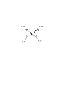
Figure 3: The quartic vertex with two vector gauge bosons and two
tensor gauge bosons - the VVTT vertex -
𝒱 α β γ γ ´ δ δ ´ a b c d ( k , p , q , r ) subscript superscript 𝒱 𝑎 𝑏 𝑐 𝑑 𝛼 𝛽 𝛾 ´ 𝛾 𝛿 ´ 𝛿 𝑘 𝑝 𝑞 𝑟 {{\cal V}}^{abcd}_{\alpha\beta\gamma\acute{\gamma}\delta\acute{\delta}}(k,p,q,r) [12 ] .
Vector gauge bosons are conventionally drawn
as thin wave lines, tensor gauge bosons are thick wave lines.
The Lorentz indices γ γ ´ 𝛾 ´ 𝛾 \gamma\acute{\gamma} q 𝑞 q δ δ ´ 𝛿 ´ 𝛿 \delta\acute{\delta} r 𝑟 r α 𝛼 \alpha k 𝑘 k β 𝛽 \beta p 𝑝 p
3 Cross section and Matrix Elements
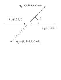
Figure 4: The scattering V + V → T + T → 𝑉 𝑉 𝑇 𝑇 V+V\rightarrow T+T k 1 , k 2 subscript 𝑘 1 subscript 𝑘 2
k_{1},k_{2} V 𝑉 V q 1 , q 2 subscript 𝑞 1 subscript 𝑞 2
q_{1},q_{2} T 𝑇 T
The scattering process is illustrated in Fig.4 k 1 μ = E ( 1 , 0 , 0 , 1 ) , k 2 μ = E ( 1 , 0 , 0 , − 1 ) , formulae-sequence superscript subscript 𝑘 1 𝜇 𝐸 1 0 0 1 superscript subscript 𝑘 2 𝜇 𝐸 1 0 0 1 k_{1}^{\mu}=E(1,0,0,1),~{}~{}k_{2}^{\mu}=E(1,0,0,-1), q 1 μ = E ( 1 , sin θ , 0 , cos θ ) , q 2 μ = E ( 1 , − s i n θ , 0 , − cos θ ) , formulae-sequence superscript subscript 𝑞 1 𝜇 𝐸 1 𝜃 0 𝜃 superscript subscript 𝑞 2 𝜇 𝐸 1 𝑠 𝑖 𝑛 𝜃 0 𝜃 q_{1}^{\mu}=E(1,\sin\theta,0,\cos\theta),~{}~{}q_{2}^{\mu}=E(1,-sin\theta,0,-\cos\theta), k 1 , 2 subscript 𝑘 1 2
k_{1,2} V + V 𝑉 𝑉 V+V q 1 , 2 subscript 𝑞 1 2
q_{1,2} T + T 𝑇 𝑇 T+T k 1 2 = k 2 2 = q 1 2 = q 2 2 = 0 superscript subscript 𝑘 1 2 superscript subscript 𝑘 2 2 subscript superscript 𝑞 2 1 subscript superscript 𝑞 2 2 0 k_{1}^{2}=k_{2}^{2}=q^{2}_{1}=q^{2}_{2}=0 k → 1 = − k → 2 subscript → 𝑘 1 subscript → 𝑘 2 \vec{k}_{1}=-\vec{k}_{2} q → 2 = − q → 1 subscript → 𝑞 2 subscript → 𝑞 1 \vec{q}_{2}=-\vec{q}_{1}
s = 2 ( k 1 ⋅ k 2 ) , t = − s 2 ( 1 − cos θ ) , u = − s 2 ( 1 + cos θ ) , formulae-sequence 𝑠 2 ⋅ subscript 𝑘 1 subscript 𝑘 2 formulae-sequence 𝑡 𝑠 2 1 𝜃 𝑢 𝑠 2 1 𝜃 \displaystyle s=2(k_{1}\cdot k_{2}),~{}~{}~{}t=-{s\over 2}(1-\cos\theta),~{}~{}~{}u=-{s\over 2}(1+\cos\theta),
where s = ( 2 E ) 2 𝑠 superscript 2 𝐸 2 s=(2E)^{2} θ 𝜃 \theta d Ω 𝑑 Ω d\Omega
d σ = 1 2 s | M | 2 1 32 π 2 d Ω , 𝑑 𝜎 1 2 𝑠 superscript 𝑀 2 1 32 superscript 𝜋 2 𝑑 Ω d\sigma={1\over 2s}|M|^{2}{1\over 32\pi^{2}}d\Omega, (13)
where the final-state density is
d Φ = 1 32 π 2 d Ω . 𝑑 Φ 1 32 superscript 𝜋 2 𝑑 Ω d\Phi={1\over 32\pi^{2}}d\Omega.
We shall calculate the polarized cross sections for the reaction V + V → T + T → 𝑉 𝑉 𝑇 𝑇 V+V\rightarrow T+T α = g 2 / 4 π 𝛼 superscript 𝑔 2 4 𝜋 \alpha=g^{2}/4\pi 5 8 g 2 superscript 𝑔 2 g^{2} V 𝑉 V T 𝑇 T
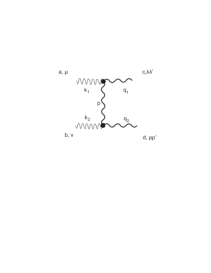
Figure 5: The t-channel diagram corresponding to the creation
of tensor gauge bosons by vector bosons V + V → T + T → 𝑉 𝑉 𝑇 𝑇 V+V\rightarrow T+T
The probability amplitude of the process can be written as a sum of four terms
corresponding to each diagram. For the first diagram Fig.5
i ℳ I a b , c d = 𝑖 superscript subscript ℳ 𝐼 𝑎 𝑏 𝑐 𝑑
absent \displaystyle i{\cal M}_{I}^{ab,cd}= (14)
= \displaystyle= 𝒱 λ λ ′ μ σ σ ′ c a e ( − q 1 , k 1 , − p ) Δ e l σ σ ′ τ τ ′ ( p ) 𝒱 τ τ ′ ν ρ ρ ′ l b d ( p , k 2 , − q 2 ) e k 1 μ e k 2 ν e q 1 ∗ λ λ ′ e q 2 ∗ ρ ρ ′ , superscript subscript 𝒱 𝜆 superscript 𝜆 ′ 𝜇 𝜎 superscript 𝜎 ′ 𝑐 𝑎 𝑒 subscript 𝑞 1 subscript 𝑘 1 𝑝 subscript superscript Δ 𝜎 superscript 𝜎 ′ 𝜏 superscript 𝜏 ′ 𝑒 𝑙 𝑝 superscript subscript 𝒱 𝜏 superscript 𝜏 ′ 𝜈 𝜌 superscript 𝜌 ′ 𝑙 𝑏 𝑑 𝑝 subscript 𝑘 2 subscript 𝑞 2 subscript superscript 𝑒 𝜇 subscript 𝑘 1 subscript superscript 𝑒 𝜈 subscript 𝑘 2 subscript superscript 𝑒 absent 𝜆 superscript 𝜆 ′ subscript 𝑞 1 subscript superscript 𝑒 absent 𝜌 superscript 𝜌 ′ subscript 𝑞 2 \displaystyle{\cal V}_{\lambda\lambda^{\prime}\mu~{}\sigma\sigma^{\prime}}^{cae}(-q_{1},k_{1},-p)~{}\Delta^{\sigma\sigma^{\prime}\tau\tau^{\prime}}_{el}(p)~{}{\cal V}_{\tau\tau^{\prime}\nu~{}\rho\rho^{\prime}}^{lbd}(p,k_{2},-q_{2})~{}e^{\mu}_{k_{1}}~{}e^{\nu}_{k_{2}}~{}e^{*\lambda\lambda^{\prime}}_{q_{1}}~{}e^{*\rho\rho^{\prime}}_{q_{2}},
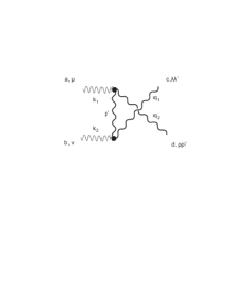
for the second diagram Fig.6
i ℳ I I a b , c d = 𝑖 superscript subscript ℳ 𝐼 𝐼 𝑎 𝑏 𝑐 𝑑
absent \displaystyle i{\cal M}_{II}^{ab,cd}= (15)
= \displaystyle= 𝒱 ρ ρ ′ μ σ σ ′ d a e ( − q 2 , k 1 , − p ′ ) Δ e l σ σ ′ τ τ ′ ( p ′ ) 𝒱 τ τ ′ ν λ λ ′ l b c ( p ′ , k 2 , − q 1 ) e k 1 μ e k 2 ν e q 1 ∗ λ λ ′ e q 2 ∗ ρ ρ ′ , superscript subscript 𝒱 𝜌 superscript 𝜌 ′ 𝜇 𝜎 superscript 𝜎 ′ 𝑑 𝑎 𝑒 subscript 𝑞 2 subscript 𝑘 1 superscript 𝑝 ′ subscript superscript Δ 𝜎 superscript 𝜎 ′ 𝜏 superscript 𝜏 ′ 𝑒 𝑙 superscript 𝑝 ′ superscript subscript 𝒱 𝜏 superscript 𝜏 ′ 𝜈 𝜆 superscript 𝜆 ′ 𝑙 𝑏 𝑐 superscript 𝑝 ′ subscript 𝑘 2 subscript 𝑞 1 subscript superscript 𝑒 𝜇 subscript 𝑘 1 subscript superscript 𝑒 𝜈 subscript 𝑘 2 subscript superscript 𝑒 absent 𝜆 superscript 𝜆 ′ subscript 𝑞 1 subscript superscript 𝑒 absent 𝜌 superscript 𝜌 ′ subscript 𝑞 2 \displaystyle{\cal V}_{\rho\rho^{\prime}\mu~{}\sigma\sigma^{\prime}}^{dae}(-q_{2},k_{1},-p^{\prime})~{}\Delta^{\sigma\sigma^{\prime}\tau\tau^{\prime}}_{el}(p^{\prime})~{}{\cal V}_{\tau\tau^{\prime}\nu~{}\lambda\lambda^{\prime}}^{lbc}(p^{\prime},k_{2},-q_{1})~{}e^{\mu}_{k_{1}}~{}e^{\nu}_{k_{2}}~{}e^{*\lambda\lambda^{\prime}}_{q_{1}}~{}e^{*\rho\rho^{\prime}}_{q_{2}},
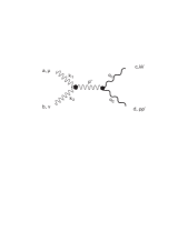
for the third diagram Fig.7
i ℳ I I I a b , c d = 𝑖 superscript subscript ℳ 𝐼 𝐼 𝐼 𝑎 𝑏 𝑐 𝑑
absent \displaystyle i{\cal M}_{III}^{ab,cd}= (16)
= \displaystyle= 𝒱 μ ν σ a b e ( k 1 , k 2 , − p ′′ ) D e l σ τ ( p ′′ ) 𝒱 λ λ ′ τ ρ ρ ′ c l d ( − q 1 , p ′′ , − q 2 ) e k 1 μ e k 2 ν e q 1 ∗ λ λ ′ e q 2 ∗ ρ ρ ′ superscript subscript 𝒱 𝜇 𝜈 𝜎 𝑎 𝑏 𝑒 subscript 𝑘 1 subscript 𝑘 2 superscript 𝑝 ′′ subscript superscript 𝐷 𝜎 𝜏 𝑒 𝑙 superscript 𝑝 ′′ superscript subscript 𝒱 𝜆 superscript 𝜆 ′ 𝜏 𝜌 superscript 𝜌 ′ 𝑐 𝑙 𝑑 subscript 𝑞 1 superscript 𝑝 ′′ subscript 𝑞 2 subscript superscript 𝑒 𝜇 subscript 𝑘 1 subscript superscript 𝑒 𝜈 subscript 𝑘 2 subscript superscript 𝑒 absent 𝜆 superscript 𝜆 ′ subscript 𝑞 1 subscript superscript 𝑒 absent 𝜌 superscript 𝜌 ′ subscript 𝑞 2 \displaystyle{\cal V}_{\mu\nu\sigma}^{abe}(k_{1},k_{2},-p^{\prime\prime})~{}D^{\sigma\tau}_{el}(p^{\prime\prime})~{}{\cal V}_{\lambda\lambda^{\prime}\tau\rho\rho^{\prime}}^{cld}(-q_{1},p^{\prime\prime},-q_{2})~{}e^{\mu}_{k_{1}}~{}e^{\nu}_{k_{2}}~{}e^{*\lambda\lambda^{\prime}}_{q_{1}}~{}e^{*\rho\rho^{\prime}}_{q_{2}}
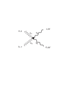
and finally for the forth diagram Fig.8
i ℳ I V a b , c d = 𝒱 μ ν ρ ρ ′ λ λ ′ a b d c ( k 1 , k 2 , − q 2 , − q 1 ) e k 1 μ e k 2 ν e q 1 ∗ λ λ ′ e q 2 ∗ ρ ρ ′ , 𝑖 superscript subscript ℳ 𝐼 𝑉 𝑎 𝑏 𝑐 𝑑
superscript subscript 𝒱 𝜇 𝜈 𝜌 superscript 𝜌 ′ 𝜆 superscript 𝜆 ′ 𝑎 𝑏 𝑑 𝑐 subscript 𝑘 1 subscript 𝑘 2 subscript 𝑞 2 subscript 𝑞 1 subscript superscript 𝑒 𝜇 subscript 𝑘 1 subscript superscript 𝑒 𝜈 subscript 𝑘 2 subscript superscript 𝑒 absent 𝜆 superscript 𝜆 ′ subscript 𝑞 1 subscript superscript 𝑒 absent 𝜌 superscript 𝜌 ′ subscript 𝑞 2 \displaystyle i{\cal M}_{IV}^{ab,cd}={\cal V}_{\mu\nu\rho\rho^{\prime}\lambda\lambda^{\prime}}^{abdc}(k_{1},k_{2},-q_{2},-q_{1})~{}e^{\mu}_{k_{1}}~{}e^{\nu}_{k_{2}}~{}e^{*\lambda\lambda^{\prime}}_{q_{1}}~{}e^{*\rho\rho^{\prime}}_{q_{2}}, (17)
where e k 1 μ subscript superscript 𝑒 𝜇 subscript 𝑘 1 e^{\mu}_{k_{1}} e k 2 ν subscript superscript 𝑒 𝜈 subscript 𝑘 2 e^{\nu}_{k_{2}} e q 1 ∗ λ λ ′ subscript superscript 𝑒 absent 𝜆 superscript 𝜆 ′ subscript 𝑞 1 e^{*\lambda\lambda^{\prime}}_{q_{1}} e q 2 ∗ ρ ρ ′ subscript superscript 𝑒 absent 𝜌 superscript 𝜌 ′ subscript 𝑞 2 e^{*\rho\rho^{\prime}}_{q_{2}}
The total amplitude is a sum of four terms:
i ℳ = i ℳ I + i ℳ I I + i ℳ I I I + i ℳ I V . 𝑖 ℳ 𝑖 subscript ℳ 𝐼 𝑖 subscript ℳ 𝐼 𝐼 𝑖 subscript ℳ 𝐼 𝐼 𝐼 𝑖 subscript ℳ 𝐼 𝑉 \displaystyle i{\cal M}=i{\cal M}_{I}+i{\cal M}_{II}+i{\cal M}_{III}+i{\cal M}_{IV}. (18)
Here we have been considering only the first nontrivial diagrams Fig.5 8 1 6
Π α α ′ β β ′ = 2 ( η α β η α ′ β ′ + η α β ′ η α ′ β − η α α ′ η β β ′ ) − 2 9 ( η α β η α ′ β ′ − η α β ′ η α ′ β ) , subscript Π 𝛼 superscript 𝛼 ′ 𝛽 superscript 𝛽 ′ 2 subscript 𝜂 𝛼 𝛽 subscript 𝜂 superscript 𝛼 ′ superscript 𝛽 ′ subscript 𝜂 𝛼 superscript 𝛽 ′ subscript 𝜂 superscript 𝛼 ′ 𝛽 subscript 𝜂 𝛼 superscript 𝛼 ′ subscript 𝜂 𝛽 superscript 𝛽 ′ 2 9 subscript 𝜂 𝛼 𝛽 subscript 𝜂 superscript 𝛼 ′ superscript 𝛽 ′ subscript 𝜂 𝛼 superscript 𝛽 ′ subscript 𝜂 superscript 𝛼 ′ 𝛽 \displaystyle\Pi_{\alpha\alpha^{\prime}\beta\beta^{\prime}}=2(\eta_{\alpha\beta}\eta_{\alpha^{\prime}\beta^{\prime}}+\eta_{\alpha\beta^{\prime}}\eta_{\alpha^{\prime}\beta}-\eta_{\alpha\alpha^{\prime}}\eta_{\beta\beta^{\prime}})-{2\over 9}(\eta_{\alpha\beta}\eta_{\alpha^{\prime}\beta^{\prime}}-\eta_{\alpha\beta^{\prime}}\eta_{\alpha^{\prime}\beta}), (19)
which, as it appears, sums the diagrams with high-rank tensor fields in the
intermediate states.
The total amplitude is gauge invariant, that is, if we take
longitudinal wave function for gauge bosons, then
the transition amplitude vanishes (see Appendix B for details).
Our intention is to calculate the physical matrix elements
in the helicity basis for initial vector and final tensor gauge bosons.
This calculation of polarized cross sections is very similar to the gluon-gluon
scattering in QCD [8 , 9 ] .
The right- and left-handed vector wave functions are:
e R ( k 1 ) μ = 1 2 ( 0 , 1 , i , 0 ) , e L ( k 1 ) μ = 1 2 ( 0 , 1 , − i , 0 ) \displaystyle e_{R}(k_{1})^{\mu}={1\over\sqrt{2}}(0,1,i,0)~{}~{}~{}~{},~{}~{}~{}~{}e_{L}(k_{1})^{\mu}={1\over\sqrt{2}}(0,1,-i,0)
e R ( k 2 ) μ = e L ( k 1 ) μ , e L ( k 2 ) μ = e R ( k 1 ) μ , \displaystyle e_{R}(k_{2})^{\mu}=e_{L}(k_{1})^{\mu}~{}~{}~{}~{},~{}~{}~{}~{}e_{L}(k_{2})^{\mu}=e_{R}(k_{1})^{\mu}, (20)
where k 1 μ = E ( 1 , 0 , 0 , 1 ) , k 2 μ = E ( 1 , 0 , 0 , − 1 ) formulae-sequence superscript subscript 𝑘 1 𝜇 𝐸 1 0 0 1 superscript subscript 𝑘 2 𝜇 𝐸 1 0 0 1 k_{1}^{\mu}=E(1,0,0,1),~{}~{}k_{2}^{\mu}=E(1,0,0,-1) q → 1 subscript → 𝑞 1 \vec{q}_{1}
e R μ α ( q 1 ) = 1 2 ( 0 , cos θ , i , − sin θ ) ⨂ ( 0 , cos θ , i , − sin θ ) , superscript subscript 𝑒 𝑅 𝜇 𝛼 subscript 𝑞 1 1 2 0 𝜃 𝑖 𝜃 tensor-product 0 𝜃 𝑖 𝜃 \displaystyle e_{R}^{\mu\alpha}(q_{1})={1\over 2}(0,\cos\theta,i,-\sin{\theta})\bigotimes(0,\cos\theta,i,-\sin{\theta}),~{}~{}~{}
e L μ α ( q 1 ) = 1 2 ( 0 , − cos θ , i , sin θ ) ⨂ ( 0 , − cos θ , i , sin θ ) superscript subscript 𝑒 𝐿 𝜇 𝛼 subscript 𝑞 1 1 2 0 𝜃 𝑖 𝜃 tensor-product 0 𝜃 𝑖 𝜃 \displaystyle e_{L}^{\mu\alpha}(q_{1})={1\over 2}(0,-\cos\theta,i,\sin{\theta})\bigotimes(0,-\cos\theta,i,\sin{\theta}) (21)
It is easy to check that the wave functions (3 e R ∗ μ α ( q 1 ) e L ( q 1 ) α ν = 0 , superscript subscript 𝑒 𝑅 absent 𝜇 𝛼 subscript 𝑞 1 subscript 𝑒 𝐿 subscript subscript 𝑞 1 𝛼 𝜈 0 e_{R}^{*\mu\alpha}(q_{1})e_{L}(q_{1})_{\alpha\nu}=0,~{} e R ∗ μ α ( q 1 ) e R ( q 1 ) μ α = 1 , superscript subscript 𝑒 𝑅 absent 𝜇 𝛼 subscript 𝑞 1 subscript 𝑒 𝑅 subscript subscript 𝑞 1 𝜇 𝛼 1 e_{R}^{*\mu\alpha}(q_{1})e_{R}(q_{1})_{\mu\alpha}=1,~{} e L ∗ μ α ( q 1 ) e L ( q 1 ) μ α = 1 superscript subscript 𝑒 𝐿 absent 𝜇 𝛼 subscript 𝑞 1 subscript 𝑒 𝐿 subscript subscript 𝑞 1 𝜇 𝛼 1 e_{L}^{*\mu\alpha}(q_{1})e_{L}(q_{1})_{\mu\alpha}=1
q 1 μ e μ α ( q 1 ) = q 1 α e μ α ( q 1 ) = 0 , q 2 μ e μ α ( q 2 ) = q 2 α e μ α ( q 2 ) = 0 , formulae-sequence subscript superscript 𝑞 𝜇 1 subscript 𝑒 𝜇 𝛼 subscript 𝑞 1 subscript superscript 𝑞 𝛼 1 subscript 𝑒 𝜇 𝛼 subscript 𝑞 1 0 subscript superscript 𝑞 𝜇 2 subscript 𝑒 𝜇 𝛼 subscript 𝑞 2 subscript superscript 𝑞 𝛼 2 subscript 𝑒 𝜇 𝛼 subscript 𝑞 2 0 \displaystyle q^{\mu}_{1}e_{\mu\alpha}(q_{1})=q^{\alpha}_{1}e_{\mu\alpha}(q_{1})=0,~{}~{}q^{\mu}_{2}e_{\mu\alpha}(q_{2})=q^{\alpha}_{2}e_{\mu\alpha}(q_{2})=0, (22)
Figure 6: The u-channel diagram for the process V + V → T + T → 𝑉 𝑉 𝑇 𝑇 V+V\rightarrow T+T
The helicity states
for the second tensor gauge boson are
e R μ ν ( q 2 ) = e L μ ν ( q 1 ) , e L μ ν ( q 2 ) = e R μ ν ( q 1 ) , formulae-sequence superscript subscript 𝑒 𝑅 𝜇 𝜈 subscript 𝑞 2 superscript subscript 𝑒 𝐿 𝜇 𝜈 subscript 𝑞 1 superscript subscript 𝑒 𝐿 𝜇 𝜈 subscript 𝑞 2 superscript subscript 𝑒 𝑅 𝜇 𝜈 subscript 𝑞 1 e_{R}^{\mu\nu}(q_{2})=e_{L}^{\mu\nu}(q_{1})~{},~{}e_{L}^{\mu\nu}(q_{2})=e_{R}^{\mu\nu}(q_{1}), q 1 μ = ( E , E sin θ , 0 , E cos θ ) superscript subscript 𝑞 1 𝜇 𝐸 𝐸 𝜃 0 𝐸 𝜃 q_{1}^{\mu}=(E,E\sin\theta,0,E\cos\theta) q 2 μ = ( E , − E sin θ , 0 , − E cos θ ) superscript subscript 𝑞 2 𝜇 𝐸 𝐸 𝜃 0 𝐸 𝜃 q_{2}^{\mu}=(E,-E\sin\theta,0,-E\cos\theta)
4 Helicity Amplitudes
Now we can calculate all sixteen matrix elements between states of definite
helicities.
The scattering amplitude (18 4 6 19 8 2 9 2 3 3 14 15 16 17
Figure 7: The s-channel diagram for the process V + V → T + T → 𝑉 𝑉 𝑇 𝑇 V+V\rightarrow T+T
For the t-channel amplitude (14 5
i ℳ I ( L L → L L ) = i ℳ I ( R R → R R ) = − g 2 3 i 4 f a c e f b d e ( 1 + cos θ ) ( 2 − cos θ ) 𝑖 subscript ℳ 𝐼 → 𝐿 𝐿 𝐿 𝐿 𝑖 subscript ℳ 𝐼 → 𝑅 𝑅 𝑅 𝑅 superscript 𝑔 2 3 𝑖 4 superscript 𝑓 𝑎 𝑐 𝑒 superscript 𝑓 𝑏 𝑑 𝑒 1 𝜃 2 𝜃 \displaystyle i{\cal M}_{I}(LL\rightarrow LL)=i{\cal M}_{I}(RR\rightarrow RR)=-g^{2}{3i\over 4}f^{ace}f^{bde}(1+\cos\theta)(2-\cos{\theta})
i ℳ I ( L L → L R ) = i ℳ I ( R R → L R ) = 0 𝑖 subscript ℳ 𝐼 → 𝐿 𝐿 𝐿 𝑅 𝑖 subscript ℳ 𝐼 → 𝑅 𝑅 𝐿 𝑅 0 \displaystyle i{\cal M}_{I}(LL\rightarrow LR)=i{\cal M}_{I}(RR\rightarrow LR)=0
i ℳ I ( L L → R L ) = i ℳ I ( R R → R L ) = 0 𝑖 subscript ℳ 𝐼 → 𝐿 𝐿 𝑅 𝐿 𝑖 subscript ℳ 𝐼 → 𝑅 𝑅 𝑅 𝐿 0 \displaystyle i{\cal M}_{I}(LL\rightarrow RL)=i{\cal M}_{I}(RR\rightarrow RL)=0
i ℳ I ( L L → R R ) = i ℳ I ( R R → L L ) = − g 2 i 8 f a c e f b d e ( 7 − 2 cos θ + cos 2 θ ) 𝑖 subscript ℳ 𝐼 → 𝐿 𝐿 𝑅 𝑅 𝑖 subscript ℳ 𝐼 → 𝑅 𝑅 𝐿 𝐿 superscript 𝑔 2 𝑖 8 superscript 𝑓 𝑎 𝑐 𝑒 superscript 𝑓 𝑏 𝑑 𝑒 7 2 𝜃 2 𝜃 \displaystyle i{\cal M}_{I}(LL\rightarrow RR)=i{\cal M}_{I}(RR\rightarrow LL)=-g^{2}{i\over 8}f^{ace}f^{bde}(7-2\cos\theta+\cos{2\theta})
i ℳ I ( L R → L L ) = i ℳ I ( L R → R R ) = − g 2 i 4 f a c e f b d e ( 1 + cos θ ) ( 3 − 2 cos θ ) 𝑖 subscript ℳ 𝐼 → 𝐿 𝑅 𝐿 𝐿 𝑖 subscript ℳ 𝐼 → 𝐿 𝑅 𝑅 𝑅 superscript 𝑔 2 𝑖 4 superscript 𝑓 𝑎 𝑐 𝑒 superscript 𝑓 𝑏 𝑑 𝑒 1 𝜃 3 2 𝜃 \displaystyle i{\cal M}_{I}(LR\rightarrow LL)=i{\cal M}_{I}(LR\rightarrow RR)=-g^{2}{i\over 4}f^{ace}f^{bde}(1+\cos\theta)(3-2\cos\theta)
i ℳ I ( L R → L R ) = 0 , i ℳ I ( L R → R L ) = 0 formulae-sequence 𝑖 subscript ℳ 𝐼 → 𝐿 𝑅 𝐿 𝑅 0 𝑖 subscript ℳ 𝐼 → 𝐿 𝑅 𝑅 𝐿 0 \displaystyle i{\cal M}_{I}(LR\rightarrow LR)=0,~{}~{}~{}~{}~{}i{\cal M}_{I}(LR\rightarrow RL)=0
i ℳ I ( R L → L L ) = i ℳ I ( R L → R R ) = − g 2 i 4 f a c e f b d e ( 1 + cos θ ) ( 3 − 2 cos θ ) 𝑖 subscript ℳ 𝐼 → 𝑅 𝐿 𝐿 𝐿 𝑖 subscript ℳ 𝐼 → 𝑅 𝐿 𝑅 𝑅 superscript 𝑔 2 𝑖 4 superscript 𝑓 𝑎 𝑐 𝑒 superscript 𝑓 𝑏 𝑑 𝑒 1 𝜃 3 2 𝜃 \displaystyle i{\cal M}_{I}(RL\rightarrow LL)=i{\cal M}_{I}(RL\rightarrow RR)=-g^{2}{i\over 4}f^{ace}f^{bde}(1+\cos\theta)(3-2\cos\theta)
i ℳ I ( R L → L R ) = 0 , i ℳ I ( R L → R L ) = 0 . formulae-sequence 𝑖 subscript ℳ 𝐼 → 𝑅 𝐿 𝐿 𝑅 0 𝑖 subscript ℳ 𝐼 → 𝑅 𝐿 𝑅 𝐿 0 \displaystyle i{\cal M}_{I}(RL\rightarrow LR)=0,~{}~{}~{}~{}~{}i{\cal M}_{I}(RL\rightarrow RL)=0. (23)
For the u-channel diagram Fig.6 15
i ℳ I I ( L L → L L ) = i ℳ I I ( R R → R R ) = − g 2 3 i 4 f a c e f b d e ( 1 − cos θ ) ( 2 + cos θ ) 𝑖 subscript ℳ 𝐼 𝐼 → 𝐿 𝐿 𝐿 𝐿 𝑖 subscript ℳ 𝐼 𝐼 → 𝑅 𝑅 𝑅 𝑅 superscript 𝑔 2 3 𝑖 4 superscript 𝑓 𝑎 𝑐 𝑒 superscript 𝑓 𝑏 𝑑 𝑒 1 𝜃 2 𝜃 \displaystyle i{\cal M}_{II}(LL\rightarrow LL)=i{\cal M}_{II}(RR\rightarrow RR)=-g^{2}{3i\over 4}f^{ace}f^{bde}(1-\cos\theta)(2+\cos{\theta})
i ℳ I I ( L L → L R ) = i ℳ I I ( R R → L R ) = 0 𝑖 subscript ℳ 𝐼 𝐼 → 𝐿 𝐿 𝐿 𝑅 𝑖 subscript ℳ 𝐼 𝐼 → 𝑅 𝑅 𝐿 𝑅 0 \displaystyle i{\cal M}_{II}(LL\rightarrow LR)=i{\cal M}_{II}(RR\rightarrow LR)=0
i ℳ I I ( L L → R L ) = i ℳ I I ( R R → R L ) = 0 𝑖 subscript ℳ 𝐼 𝐼 → 𝐿 𝐿 𝑅 𝐿 𝑖 subscript ℳ 𝐼 𝐼 → 𝑅 𝑅 𝑅 𝐿 0 \displaystyle i{\cal M}_{II}(LL\rightarrow RL)=i{\cal M}_{II}(RR\rightarrow RL)=0
i ℳ I I ( L L → R R ) = i ℳ I I ( R R → L L ) = − g 2 i 8 f a d e f b c e ( 7 + 2 cos θ − cos 2 θ ) 𝑖 subscript ℳ 𝐼 𝐼 → 𝐿 𝐿 𝑅 𝑅 𝑖 subscript ℳ 𝐼 𝐼 → 𝑅 𝑅 𝐿 𝐿 superscript 𝑔 2 𝑖 8 superscript 𝑓 𝑎 𝑑 𝑒 superscript 𝑓 𝑏 𝑐 𝑒 7 2 𝜃 2 𝜃 \displaystyle i{\cal M}_{II}(LL\rightarrow RR)=i{\cal M}_{II}(RR\rightarrow LL)=-g^{2}{i\over 8}f^{ade}f^{bce}(7+2\cos\theta-\cos{2\theta})
i ℳ I I ( L R → L L ) = i ℳ I I ( L R → R R ) = − g 2 i 4 f a d e f b c e ( 1 − cos θ ) ( 3 + 2 cos θ ) 𝑖 subscript ℳ 𝐼 𝐼 → 𝐿 𝑅 𝐿 𝐿 𝑖 subscript ℳ 𝐼 𝐼 → 𝐿 𝑅 𝑅 𝑅 superscript 𝑔 2 𝑖 4 superscript 𝑓 𝑎 𝑑 𝑒 superscript 𝑓 𝑏 𝑐 𝑒 1 𝜃 3 2 𝜃 \displaystyle i{\cal M}_{II}(LR\rightarrow LL)=i{\cal M}_{II}(LR\rightarrow RR)=-g^{2}{i\over 4}f^{ade}f^{bce}(1-\cos\theta)(3+2\cos\theta)
i ℳ I I ( L R → L R ) = 0 , i ℳ I I ( L R → R L ) = 0 formulae-sequence 𝑖 subscript ℳ 𝐼 𝐼 → 𝐿 𝑅 𝐿 𝑅 0 𝑖 subscript ℳ 𝐼 𝐼 → 𝐿 𝑅 𝑅 𝐿 0 \displaystyle i{\cal M}_{II}(LR\rightarrow LR)=0,~{}~{}~{}~{}~{}i{\cal M}_{II}(LR\rightarrow RL)=0
i ℳ I I ( R L → L L ) = i ℳ I I ( R L → R R ) = − g 2 i 4 f a d e f b c e ( 1 − cos θ ) ( 3 + 2 cos θ ) 𝑖 subscript ℳ 𝐼 𝐼 → 𝑅 𝐿 𝐿 𝐿 𝑖 subscript ℳ 𝐼 𝐼 → 𝑅 𝐿 𝑅 𝑅 superscript 𝑔 2 𝑖 4 superscript 𝑓 𝑎 𝑑 𝑒 superscript 𝑓 𝑏 𝑐 𝑒 1 𝜃 3 2 𝜃 \displaystyle i{\cal M}_{II}(RL\rightarrow LL)=i{\cal M}_{II}(RL\rightarrow RR)=-g^{2}{i\over 4}f^{ade}f^{bce}(1-\cos\theta)(3+2\cos\theta)
i ℳ I I ( R L → L R ) = 0 , i ℳ I I ( R L → R L ) = 0 . formulae-sequence 𝑖 subscript ℳ 𝐼 𝐼 → 𝑅 𝐿 𝐿 𝑅 0 𝑖 subscript ℳ 𝐼 𝐼 → 𝑅 𝐿 𝑅 𝐿 0 \displaystyle i{\cal M}_{II}(RL\rightarrow LR)=0,~{}~{}~{}~{}~{}i{\cal M}_{II}(RL\rightarrow RL)=0. (24)
For the s-channel diagram Fig.7 16
i ℳ I I I ( L L → L L ) = i ℳ I I I ( R R → R R ) = − g 2 i 2 ( f a c e f b d e − f a d e f b c e ) cos θ 𝑖 subscript ℳ 𝐼 𝐼 𝐼 → 𝐿 𝐿 𝐿 𝐿 𝑖 subscript ℳ 𝐼 𝐼 𝐼 → 𝑅 𝑅 𝑅 𝑅 superscript 𝑔 2 𝑖 2 superscript 𝑓 𝑎 𝑐 𝑒 superscript 𝑓 𝑏 𝑑 𝑒 superscript 𝑓 𝑎 𝑑 𝑒 superscript 𝑓 𝑏 𝑐 𝑒 𝜃 \displaystyle i{\cal M}_{III}(LL\rightarrow LL)=i{\cal M}_{III}(RR\rightarrow RR)=-g^{2}{i\over 2}(f^{ace}f^{bde}-f^{ade}f^{bce})\cos{\theta}
i ℳ I I I ( L L → L R ) = i ℳ I I I ( R R → L R ) = 0 𝑖 subscript ℳ 𝐼 𝐼 𝐼 → 𝐿 𝐿 𝐿 𝑅 𝑖 subscript ℳ 𝐼 𝐼 𝐼 → 𝑅 𝑅 𝐿 𝑅 0 \displaystyle i{\cal M}_{III}(LL\rightarrow LR)=i{\cal M}_{III}(RR\rightarrow LR)=0
i ℳ I I I ( L L → R L ) = i ℳ I I I ( R R → R L ) = 0 𝑖 subscript ℳ 𝐼 𝐼 𝐼 → 𝐿 𝐿 𝑅 𝐿 𝑖 subscript ℳ 𝐼 𝐼 𝐼 → 𝑅 𝑅 𝑅 𝐿 0 \displaystyle i{\cal M}_{III}(LL\rightarrow RL)=i{\cal M}_{III}(RR\rightarrow RL)=0
i ℳ I I I ( L L → R R ) = i ℳ I I I ( R R → L L ) = − g 2 i 2 ( f a c e f b d e − f a d e f b c e ) cos θ 𝑖 subscript ℳ 𝐼 𝐼 𝐼 → 𝐿 𝐿 𝑅 𝑅 𝑖 subscript ℳ 𝐼 𝐼 𝐼 → 𝑅 𝑅 𝐿 𝐿 superscript 𝑔 2 𝑖 2 superscript 𝑓 𝑎 𝑐 𝑒 superscript 𝑓 𝑏 𝑑 𝑒 superscript 𝑓 𝑎 𝑑 𝑒 superscript 𝑓 𝑏 𝑐 𝑒 𝜃 \displaystyle i{\cal M}_{III}(LL\rightarrow RR)=i{\cal M}_{III}(RR\rightarrow LL)=-g^{2}{i\over 2}(f^{ace}f^{bde}-f^{ade}f^{bce})\cos{\theta}
i ℳ I I I ( L R → L L ) = i ℳ I I I ( L R → R R ) = 0 𝑖 subscript ℳ 𝐼 𝐼 𝐼 → 𝐿 𝑅 𝐿 𝐿 𝑖 subscript ℳ 𝐼 𝐼 𝐼 → 𝐿 𝑅 𝑅 𝑅 0 \displaystyle i{\cal M}_{III}(LR\rightarrow LL)=i{\cal M}_{III}(LR\rightarrow RR)=0
i ℳ I I I ( L R → L R ) = 0 , i ℳ I I I ( L R → R L ) = 0 formulae-sequence 𝑖 subscript ℳ 𝐼 𝐼 𝐼 → 𝐿 𝑅 𝐿 𝑅 0 𝑖 subscript ℳ 𝐼 𝐼 𝐼 → 𝐿 𝑅 𝑅 𝐿 0 \displaystyle i{\cal M}_{III}(LR\rightarrow LR)=0,~{}~{}~{}~{}~{}i{\cal M}_{III}(LR\rightarrow RL)=0
i ℳ I I I ( R L → L L ) = i ℳ I I I ( R L → R R ) = 0 𝑖 subscript ℳ 𝐼 𝐼 𝐼 → 𝑅 𝐿 𝐿 𝐿 𝑖 subscript ℳ 𝐼 𝐼 𝐼 → 𝑅 𝐿 𝑅 𝑅 0 \displaystyle i{\cal M}_{III}(RL\rightarrow LL)=i{\cal M}_{III}(RL\rightarrow RR)=0
i ℳ I I I ( R L → L R ) = 0 , i ℳ I I I ( R L → R L ) = 0 . formulae-sequence 𝑖 subscript ℳ 𝐼 𝐼 𝐼 → 𝑅 𝐿 𝐿 𝑅 0 𝑖 subscript ℳ 𝐼 𝐼 𝐼 → 𝑅 𝐿 𝑅 𝐿 0 \displaystyle i{\cal M}_{III}(RL\rightarrow LR)=0,~{}~{}~{}~{}~{}i{\cal M}_{III}(RL\rightarrow RL)=0. (25)
Figure 8: The contact diagram for the process V + V → T + T → 𝑉 𝑉 𝑇 𝑇 V+V\rightarrow T+T
And finally for the contact diagram Fig.8 17
i ℳ I V ( L L → L L ) = i ℳ I V ( R R → R R ) = g 2 i 4 ( f a c e f b d e + f a d e f b c e ) sin 2 θ 𝑖 subscript ℳ 𝐼 𝑉 → 𝐿 𝐿 𝐿 𝐿 𝑖 subscript ℳ 𝐼 𝑉 → 𝑅 𝑅 𝑅 𝑅 superscript 𝑔 2 𝑖 4 superscript 𝑓 𝑎 𝑐 𝑒 superscript 𝑓 𝑏 𝑑 𝑒 superscript 𝑓 𝑎 𝑑 𝑒 superscript 𝑓 𝑏 𝑐 𝑒 superscript 2 𝜃 \displaystyle i{\cal M}_{IV}(LL\rightarrow LL)=i{\cal M}_{IV}(RR\rightarrow RR)=g^{2}{i\over 4}(f^{ace}f^{bde}+f^{ade}f^{bce})\sin^{2}\theta
i ℳ I V ( L L → L R ) = i ℳ I V ( R R → L R ) = 0 𝑖 subscript ℳ 𝐼 𝑉 → 𝐿 𝐿 𝐿 𝑅 𝑖 subscript ℳ 𝐼 𝑉 → 𝑅 𝑅 𝐿 𝑅 0 \displaystyle i{\cal M}_{IV}(LL\rightarrow LR)=i{\cal M}_{IV}(RR\rightarrow LR)=0
i ℳ I V ( L L → R L ) = i ℳ I V ( R R → R L ) = 0 𝑖 subscript ℳ 𝐼 𝑉 → 𝐿 𝐿 𝑅 𝐿 𝑖 subscript ℳ 𝐼 𝑉 → 𝑅 𝑅 𝑅 𝐿 0 \displaystyle i{\cal M}_{IV}(LL\rightarrow RL)=i{\cal M}_{IV}(RR\rightarrow RL)=0
i ℳ I V ( L L → R R ) = i ℳ I V ( R R → L L ) = g 2 i 4 ( f a c e f b d e + f a d e f b c e ) sin 2 θ 𝑖 subscript ℳ 𝐼 𝑉 → 𝐿 𝐿 𝑅 𝑅 𝑖 subscript ℳ 𝐼 𝑉 → 𝑅 𝑅 𝐿 𝐿 superscript 𝑔 2 𝑖 4 superscript 𝑓 𝑎 𝑐 𝑒 superscript 𝑓 𝑏 𝑑 𝑒 superscript 𝑓 𝑎 𝑑 𝑒 superscript 𝑓 𝑏 𝑐 𝑒 superscript 2 𝜃 \displaystyle i{\cal M}_{IV}(LL\rightarrow RR)=i{\cal M}_{IV}(RR\rightarrow LL)=g^{2}{i\over 4}(f^{ace}f^{bde}+f^{ade}f^{bce})\sin^{2}\theta
i ℳ I V ( L R → L L ) = i ℳ I V ( L R → R R ) = g 2 i 4 ( f a c e f b d e + f a d e f b c e ) sin 2 θ 𝑖 subscript ℳ 𝐼 𝑉 → 𝐿 𝑅 𝐿 𝐿 𝑖 subscript ℳ 𝐼 𝑉 → 𝐿 𝑅 𝑅 𝑅 superscript 𝑔 2 𝑖 4 superscript 𝑓 𝑎 𝑐 𝑒 superscript 𝑓 𝑏 𝑑 𝑒 superscript 𝑓 𝑎 𝑑 𝑒 superscript 𝑓 𝑏 𝑐 𝑒 superscript 2 𝜃 \displaystyle i{\cal M}_{IV}(LR\rightarrow LL)=i{\cal M}_{IV}(LR\rightarrow RR)=g^{2}{i\over 4}(f^{ace}f^{bde}+f^{ade}f^{bce})\sin^{2}\theta
i ℳ I V ( L R → L R ) = 0 , i ℳ I V ( L R → R L ) = 0 formulae-sequence 𝑖 subscript ℳ 𝐼 𝑉 → 𝐿 𝑅 𝐿 𝑅 0 𝑖 subscript ℳ 𝐼 𝑉 → 𝐿 𝑅 𝑅 𝐿 0 \displaystyle i{\cal M}_{IV}(LR\rightarrow LR)=0,~{}~{}~{}~{}~{}i{\cal M}_{IV}(LR\rightarrow RL)=0
i ℳ I V ( R L → L L ) = i ℳ I V ( R L → R R ) = g 2 i 4 ( f a c e f b d e + f a d e f b c e ) sin 2 θ 𝑖 subscript ℳ 𝐼 𝑉 → 𝑅 𝐿 𝐿 𝐿 𝑖 subscript ℳ 𝐼 𝑉 → 𝑅 𝐿 𝑅 𝑅 superscript 𝑔 2 𝑖 4 superscript 𝑓 𝑎 𝑐 𝑒 superscript 𝑓 𝑏 𝑑 𝑒 superscript 𝑓 𝑎 𝑑 𝑒 superscript 𝑓 𝑏 𝑐 𝑒 superscript 2 𝜃 \displaystyle i{\cal M}_{IV}(RL\rightarrow LL)=i{\cal M}_{IV}(RL\rightarrow RR)=g^{2}{i\over 4}(f^{ace}f^{bde}+f^{ade}f^{bce})\sin^{2}\theta
i ℳ I V ( R L → L R ) = 0 , i ℳ I V ( R L → R L ) = 0 . formulae-sequence 𝑖 subscript ℳ 𝐼 𝑉 → 𝑅 𝐿 𝐿 𝑅 0 𝑖 subscript ℳ 𝐼 𝑉 → 𝑅 𝐿 𝑅 𝐿 0 \displaystyle i{\cal M}_{IV}(RL\rightarrow LR)=0,~{}~{}~{}~{}~{}~{}i{\cal M}_{IV}(RL\rightarrow RL)=0. (26)
Thus only eight amplitudes out of sixteen are nonzero:
V L V L → T L T L , V R V R → T R T R , V L V L → T R T R , V R V R → T L T L , V L V R → T L T L , V L V R → T R T R , V R V L → T L T L , V R V L → T R T R . formulae-sequence → subscript 𝑉 𝐿 subscript 𝑉 𝐿 subscript 𝑇 𝐿 subscript 𝑇 𝐿 formulae-sequence → subscript 𝑉 𝑅 subscript 𝑉 𝑅 subscript 𝑇 𝑅 subscript 𝑇 𝑅 formulae-sequence → subscript 𝑉 𝐿 subscript 𝑉 𝐿 subscript 𝑇 𝑅 subscript 𝑇 𝑅 formulae-sequence → subscript 𝑉 𝑅 subscript 𝑉 𝑅 subscript 𝑇 𝐿 subscript 𝑇 𝐿 formulae-sequence → subscript 𝑉 𝐿 subscript 𝑉 𝑅 subscript 𝑇 𝐿 subscript 𝑇 𝐿 formulae-sequence → subscript 𝑉 𝐿 subscript 𝑉 𝑅 subscript 𝑇 𝑅 subscript 𝑇 𝑅 formulae-sequence → subscript 𝑉 𝑅 subscript 𝑉 𝐿 subscript 𝑇 𝐿 subscript 𝑇 𝐿 → subscript 𝑉 𝑅 subscript 𝑉 𝐿 subscript 𝑇 𝑅 subscript 𝑇 𝑅 V_{L}V_{L}\rightarrow T_{L}T_{L},~{}~{}V_{R}V_{R}\rightarrow T_{R}T_{R},~{}~{}V_{L}V_{L}\rightarrow T_{R}T_{R},~{}~{}V_{R}V_{R}\rightarrow T_{L}T_{L},~{}~{}V_{L}V_{R}\rightarrow T_{L}T_{L},~{}~{}V_{L}V_{R}\rightarrow T_{R}T_{R},~{}~{}V_{R}V_{L}\rightarrow T_{L}T_{L},~{}~{}V_{R}V_{L}\rightarrow T_{R}T_{R}. 18
i ℳ L L → L L = − i g 2 4 [ \displaystyle i{\cal M}_{LL\rightarrow LL}=-{ig^{2}\over 4}\biggl{[} + \displaystyle+ f a c e f b d e ( 4 + 5 cos θ + cos 2 θ ) + limit-from superscript 𝑓 𝑎 𝑐 𝑒 superscript 𝑓 𝑏 𝑑 𝑒 4 5 𝜃 2 𝜃 \displaystyle f^{ace}f^{bde}(4+5\cos\theta+\cos{2\theta})+ (27)
+ \displaystyle+ f a d e f b c e ( 4 − 5 cos θ + cos 2 θ ) ] , \displaystyle f^{ade}f^{bce}(4-5\cos\theta+\cos{2\theta})\biggr{]},
i ℳ L L → R R = − i g 2 4 [ f a c e f b d e ( 3 + cos θ ) + f a d e f b c e ( 3 − cos θ ) ] , 𝑖 subscript ℳ → 𝐿 𝐿 𝑅 𝑅 𝑖 superscript 𝑔 2 4 delimited-[] superscript 𝑓 𝑎 𝑐 𝑒 superscript 𝑓 𝑏 𝑑 𝑒 3 𝜃 superscript 𝑓 𝑎 𝑑 𝑒 superscript 𝑓 𝑏 𝑐 𝑒 3 𝜃 \displaystyle i{\cal M}_{LL\rightarrow RR}=-{ig^{2}\over 4}\biggl{[}f^{ace}f^{bde}(3+\cos\theta)+f^{ade}f^{bce}(3-\cos\theta)\biggr{]}, (28)
i ℳ L R → L L = − i g 2 4 [ \displaystyle i{\cal M}_{LR\rightarrow LL}=-{ig^{2}\over 4}\biggl{[} + ( 1 + cos θ ) ( 2 − cos θ ) f a c e f b d e + limit-from 1 𝜃 2 𝜃 superscript 𝑓 𝑎 𝑐 𝑒 superscript 𝑓 𝑏 𝑑 𝑒 \displaystyle+(1+\cos\theta)(2-\cos\theta)f^{ace}f^{bde}+ (29)
+ ( 1 − cos θ ) ( 2 + cos θ ) f a d e f b c e ] . \displaystyle+(1-\cos\theta)(2+\cos\theta)f^{ade}f^{bce}\biggr{]}.
To compute the cross section, we must square matrix elements
(27 28 29
1 d ( G ) 2 ∑ c o l | ℳ L L → L L | 2 = g 4 32 C 2 2 ( G ) d ( G ) ( 124 − 23 cos 2 θ + 3 cos 4 θ ) , 1 𝑑 superscript 𝐺 2 subscript 𝑐 𝑜 𝑙 superscript subscript ℳ → 𝐿 𝐿 𝐿 𝐿 2 superscript 𝑔 4 32 superscript subscript 𝐶 2 2 𝐺 𝑑 𝐺 124 23 2 𝜃 3 4 𝜃 \displaystyle{1\over d(G)^{2}}\sum_{col}|{\cal M}_{LL\rightarrow LL}|^{2}=~{}{g^{4}\over 32}~{}{C_{2}^{2}(G)\over d(G)}(124-23\cos{2\theta}+3\cos{4\theta}), (30)
1 d ( G ) 2 ∑ c o l | ℳ L L → R R | 2 = g 4 32 C 2 2 ( G ) d ( G ) ( 55 + cos 2 θ ) , 1 𝑑 superscript 𝐺 2 subscript 𝑐 𝑜 𝑙 superscript subscript ℳ → 𝐿 𝐿 𝑅 𝑅 2 superscript 𝑔 4 32 superscript subscript 𝐶 2 2 𝐺 𝑑 𝐺 55 2 𝜃 \displaystyle{1\over d(G)^{2}}\sum_{col}|{\cal M}_{LL\rightarrow RR}|^{2}=~{}{g^{4}\over 32}~{}{C_{2}^{2}(G)\over d(G)}(55+\cos{2\theta}), (31)
1 d ( G ) 2 ∑ c o l | ℳ L R → L L | 2 = g 4 128 C 2 2 ( G ) d ( G ) ( 61 − 32 cos 2 θ + 3 cos 4 θ ) , 1 𝑑 superscript 𝐺 2 subscript 𝑐 𝑜 𝑙 superscript subscript ℳ → 𝐿 𝑅 𝐿 𝐿 2 superscript 𝑔 4 128 superscript subscript 𝐶 2 2 𝐺 𝑑 𝐺 61 32 2 𝜃 3 4 𝜃 \displaystyle{1\over d(G)^{2}}\sum_{col}|{\cal M}_{LR\rightarrow LL}|^{2}=~{}{g^{4}\over 128}~{}{C_{2}^{2}(G)\over d(G)}(61-32\cos{2\theta}+3\cos{4\theta}), (32)
where the invariant operator C 2 subscript 𝐶 2 C_{2} t a t a = C 2 1 superscript 𝑡 𝑎 superscript 𝑡 𝑎 subscript 𝐶 2 1 t^{a}t^{a}=C_{2}~{}1 V + V → T + T → 𝑉 𝑉 𝑇 𝑇 V+V\rightarrow T+T Helicity cross-sections.
Plugging matrix elements (30 31 32 13
d σ L L → L L = α 2 s C 2 2 ( G ) 128 d ( G ) ( 124 − 23 cos 2 θ + 3 cos 4 θ ) d Ω , 𝑑 subscript 𝜎 → 𝐿 𝐿 𝐿 𝐿 superscript 𝛼 2 𝑠 subscript superscript 𝐶 2 2 𝐺 128 𝑑 𝐺 124 23 2 𝜃 3 4 𝜃 𝑑 Ω \displaystyle d\sigma_{LL\rightarrow LL}={\alpha^{2}\over s}~{}{C^{2}_{2}(G)\over 128d(G)}~{}~{}(124-23\cos{2\theta}+3\cos{4\theta})~{}d\Omega, (33)
d σ L L → R R = α 2 s C 2 2 ( G ) 128 d ( G ) ( 55 + cos 2 θ ) d Ω , 𝑑 subscript 𝜎 → 𝐿 𝐿 𝑅 𝑅 superscript 𝛼 2 𝑠 subscript superscript 𝐶 2 2 𝐺 128 𝑑 𝐺 55 2 𝜃 𝑑 Ω \displaystyle d\sigma_{LL\rightarrow RR}={\alpha^{2}\over s}~{}{C^{2}_{2}(G)\over 128d(G)}~{}~{}(55+\cos{2\theta})~{}d\Omega, (34)
d σ L R → L L = α 2 s C 2 2 ( G ) 512 d ( G ) ( 61 − 32 cos 2 θ + 3 cos 4 θ ) d Ω , 𝑑 subscript 𝜎 → 𝐿 𝑅 𝐿 𝐿 superscript 𝛼 2 𝑠 subscript superscript 𝐶 2 2 𝐺 512 𝑑 𝐺 61 32 2 𝜃 3 4 𝜃 𝑑 Ω \displaystyle d\sigma_{LR\rightarrow LL}={\alpha^{2}\over s}~{}{C^{2}_{2}(G)\over 512d(G)}~{}~{}(61-32\cos{2\theta}+3\cos{4\theta})~{}d\Omega, (35)
where
α = g 2 4 π . 𝛼 superscript 𝑔 2 4 𝜋 \alpha={g^{2}\over 4\pi}. Unpolarized cross section.
Adding up all sixteen helicity amplitudes and dividing the result
by four in order to average over the initial boson spins we can get
unpolarized cross section. Thus summing over helicities
1 4 d ( G ) 2 ∑ c o l , h e l | ℳ | 2 = 1 4 d ( G ) 2 ∑ c o l 2 | ℳ L L → L L | 2 + 2 | ℳ L L → R R | 2 + 4 | ℳ L R → R R | 2 = 1 4 𝑑 superscript 𝐺 2 subscript 𝑐 𝑜 𝑙 ℎ 𝑒 𝑙
superscript ℳ 2 1 4 𝑑 superscript 𝐺 2 subscript 𝑐 𝑜 𝑙 2 superscript subscript ℳ → 𝐿 𝐿 𝐿 𝐿 2 2 superscript subscript ℳ → 𝐿 𝐿 𝑅 𝑅 2 4 superscript subscript ℳ → 𝐿 𝑅 𝑅 𝑅 2 absent \displaystyle{1\over 4d(G)^{2}}\sum_{col,hel}|{\cal M}|^{2}={1\over 4d(G)^{2}}\sum_{col}2|{\cal M}_{LL\rightarrow LL}|^{2}+2|{\cal M}_{LL\rightarrow RR}|^{2}+4|{\cal M}_{LR\rightarrow RR}|^{2}=
= g 2 2 g 4 128 C 2 2 ( G ) d ( G ) ( 419 − 76 cos 2 θ + 9 cos 4 θ ) absent superscript subscript 𝑔 2 2 superscript 𝑔 4 128 superscript subscript 𝐶 2 2 𝐺 𝑑 𝐺 419 76 2 𝜃 9 4 𝜃 \displaystyle=g_{2}^{2}{g^{4}\over 128}{C_{2}^{2}(G)\over d(G)}\biggl{(}~{}419-76\cos{2\theta}+9\cos{4\theta}~{}\biggr{)} (36)
for unpolarized cross section we shall get
d σ = α 2 s C 2 2 ( G ) d ( G ) 419 − 76 cos 2 θ + 9 cos 4 θ 512 d Ω , 𝑑 𝜎 superscript 𝛼 2 𝑠 subscript superscript 𝐶 2 2 𝐺 𝑑 𝐺 419 76 2 𝜃 9 4 𝜃 512 𝑑 Ω \displaystyle d\sigma={\alpha^{2}\over s}~{}{C^{2}_{2}(G)\over d(G)}~{}~{}{419-76\cos{2\theta}+9\cos{4\theta}\over 512}~{}d\Omega, (37)
where for the S U ( N ) 𝑆 𝑈 𝑁 SU(N) C 2 2 ( G ) d ( G ) = N 2 ( N 2 − 1 ) subscript superscript 𝐶 2 2 𝐺 𝑑 𝐺 superscript 𝑁 2 superscript 𝑁 2 1 {C^{2}_{2}(G)\over d(G)}~{}~{}=~{}{N^{2}\over(N^{2}-1)} 37 θ = π / 2 𝜃 𝜋 2 \theta=\pi/2
This cross section should be compared with the analogous cross section
in QCD. Indeed, let us compare this result with the gluon-gluon scattering [9 ] .
The V + V → V + V → 𝑉 𝑉 𝑉 𝑉 V+V\rightarrow V+V
d σ = α 2 s C 2 2 ( G ) d ( G ) ( 4 − s i n 2 θ ) 3 32 sin 4 θ d Ω . 𝑑 𝜎 superscript 𝛼 2 𝑠 superscript subscript 𝐶 2 2 𝐺 𝑑 𝐺 superscript 4 𝑠 𝑖 superscript 𝑛 2 𝜃 3 32 superscript 4 𝜃 𝑑 Ω \displaystyle d\sigma={\alpha^{2}\over s}~{}{C_{2}^{2}(G)\over d(G)}~{}{(4-sin^{2}\theta)^{3}\over 32\sin^{4}\theta}~{}d\Omega. (38)
This cross section increases at small angles θ ∼ 0 , π similar-to 𝜃 0 𝜋
\theta\sim 0,\pi θ = π / 2 𝜃 𝜋 2 \theta=\pi/2 37 θ = π / 2 𝜃 𝜋 2 \theta=\pi/2
5 Appendix A
Here we shall review the well known result for the three-level gluon scattering
V + V → V + V → 𝑉 𝑉 𝑉 𝑉 V+V\rightarrow V+V [9 ] in order to compare it with the tensor scattering
considered above: V + V → T + T → 𝑉 𝑉 𝑇 𝑇 V+V\rightarrow T+T
i ℳ ( L L → L L ) = i ℳ ( R R → R R ) , i ℳ ( L L → R R ) = i ℳ ( R R → L L ) , formulae-sequence 𝑖 ℳ → 𝐿 𝐿 𝐿 𝐿 𝑖 ℳ → 𝑅 𝑅 𝑅 𝑅 𝑖 ℳ → 𝐿 𝐿 𝑅 𝑅 𝑖 ℳ → 𝑅 𝑅 𝐿 𝐿 \displaystyle i{\cal M}(LL\rightarrow LL)=i{\cal M}(RR\rightarrow RR),~{}~{}~{}i{\cal M}(LL\rightarrow RR)=i{\cal M}(RR\rightarrow LL),
i ℳ ( L L → L R ) = i ℳ ( R R → L R ) = i ℳ ( L R → L L ) = i ℳ ( L R → R R ) = 𝑖 ℳ → 𝐿 𝐿 𝐿 𝑅 𝑖 ℳ → 𝑅 𝑅 𝐿 𝑅 𝑖 ℳ → 𝐿 𝑅 𝐿 𝐿 𝑖 ℳ → 𝐿 𝑅 𝑅 𝑅 absent \displaystyle i{\cal M}(LL\rightarrow LR)=i{\cal M}(RR\rightarrow LR)=i{\cal M}(LR\rightarrow LL)=i{\cal M}(LR\rightarrow RR)=
= \displaystyle= i ℳ ( L L → R L ) = i ℳ ( R R → R L ) = i ℳ ( R L → L L ) = i ℳ ( R L → R R ) , 𝑖 ℳ → 𝐿 𝐿 𝑅 𝐿 𝑖 ℳ → 𝑅 𝑅 𝑅 𝐿 𝑖 ℳ → 𝑅 𝐿 𝐿 𝐿 𝑖 ℳ → 𝑅 𝐿 𝑅 𝑅 \displaystyle i{\cal M}(LL\rightarrow RL)=i{\cal M}(RR\rightarrow RL)=i{\cal M}(RL\rightarrow LL)=i{\cal M}(RL\rightarrow RR),
i ℳ ( L R → L R ) = i ℳ ( R L → R L ) , i ℳ ( L R → R L ) = i ℳ ( R L → L R ) . formulae-sequence 𝑖 ℳ → 𝐿 𝑅 𝐿 𝑅 𝑖 ℳ → 𝑅 𝐿 𝑅 𝐿 𝑖 ℳ → 𝐿 𝑅 𝑅 𝐿 𝑖 ℳ → 𝑅 𝐿 𝐿 𝑅 \displaystyle i{\cal M}(LR\rightarrow LR)=i{\cal M}(RL\rightarrow RL),~{}~{}~{}i{\cal M}(LR\rightarrow RL)=i{\cal M}(RL\rightarrow LR).
Four Feynman diagram contribute into this scattering. The contribution
of the t-channel diagram can be expressed in the form:
i ℳ I ( L L → L L ) = i g 2 8 f a c e f b d e ( 39 − 24 cos θ + cos 2 θ ) cot 2 θ 2 𝑖 subscript ℳ 𝐼 → 𝐿 𝐿 𝐿 𝐿 𝑖 superscript 𝑔 2 8 superscript 𝑓 𝑎 𝑐 𝑒 superscript 𝑓 𝑏 𝑑 𝑒 39 24 𝜃 2 𝜃 superscript 2 𝜃 2 \displaystyle i{\cal M}_{I}(LL\rightarrow LL)={ig^{2}\over 8}f^{ace}f^{bde}(39-24\cos\theta+\cos{2\theta})\cot^{2}{\theta\over 2}
i ℳ I ( L L → L R ) = i g 2 4 f a c e f b d e sin 2 θ 𝑖 subscript ℳ 𝐼 → 𝐿 𝐿 𝐿 𝑅 𝑖 superscript 𝑔 2 4 superscript 𝑓 𝑎 𝑐 𝑒 superscript 𝑓 𝑏 𝑑 𝑒 superscript 2 𝜃 \displaystyle i{\cal M}_{I}(LL\rightarrow LR)={ig^{2}\over 4}f^{ace}f^{bde}\sin^{2}\theta
i ℳ I ( L L → R R ) = i g 2 2 f a c e f b d e ( 3 + cos θ sin 2 θ 2 ) sin 4 θ 2 𝑖 subscript ℳ 𝐼 → 𝐿 𝐿 𝑅 𝑅 𝑖 superscript 𝑔 2 2 superscript 𝑓 𝑎 𝑐 𝑒 superscript 𝑓 𝑏 𝑑 𝑒 3 𝜃 superscript 2 𝜃 2 superscript 4 𝜃 2 \displaystyle i{\cal M}_{I}(LL\rightarrow RR)={ig^{2}\over 2}f^{ace}f^{bde}\biggl{(}{3+\cos\theta\over\sin^{2}{\theta\over 2}}\biggr{)}\sin^{4}{\theta\over 2}
i ℳ I ( L R → L R ) = i g 2 2 f a c e f b d e ( 3 + cos θ sin 2 θ 2 ) cos 4 θ 2 𝑖 subscript ℳ 𝐼 → 𝐿 𝑅 𝐿 𝑅 𝑖 superscript 𝑔 2 2 superscript 𝑓 𝑎 𝑐 𝑒 superscript 𝑓 𝑏 𝑑 𝑒 3 𝜃 superscript 2 𝜃 2 superscript 4 𝜃 2 \displaystyle i{\cal M}_{I}(LR\rightarrow LR)={ig^{2}\over 2}f^{ace}f^{bde}\biggl{(}{3+\cos\theta\over\sin^{2}{\theta\over 2}}\biggr{)}\cos^{4}{\theta\over 2}
i ℳ I ( L R → R L ) = i g 2 2 f a c e f b d e ( 3 + cos θ sin 2 θ 2 ) sin 4 θ 2 , 𝑖 subscript ℳ 𝐼 → 𝐿 𝑅 𝑅 𝐿 𝑖 superscript 𝑔 2 2 superscript 𝑓 𝑎 𝑐 𝑒 superscript 𝑓 𝑏 𝑑 𝑒 3 𝜃 superscript 2 𝜃 2 superscript 4 𝜃 2 \displaystyle i{\cal M}_{I}(LR\rightarrow RL)={ig^{2}\over 2}f^{ace}f^{bde}\biggl{(}{3+\cos\theta\over\sin^{2}{\theta\over 2}}\biggr{)}\sin^{4}{\theta\over 2}, (39)
of the u-channel diagram as
i ℳ I I ( L L → L L ) = i g 2 8 f a d e f b c e ( 39 + 24 cos θ + cos 2 θ ) tan 2 θ 2 𝑖 subscript ℳ 𝐼 𝐼 → 𝐿 𝐿 𝐿 𝐿 𝑖 superscript 𝑔 2 8 superscript 𝑓 𝑎 𝑑 𝑒 superscript 𝑓 𝑏 𝑐 𝑒 39 24 𝜃 2 𝜃 superscript 2 𝜃 2 \displaystyle i{\cal M}_{II}(LL\rightarrow LL)={ig^{2}\over 8}f^{ade}f^{bce}(39+24\cos\theta+\cos{2\theta})\tan^{2}{\theta\over 2}
i ℳ I I ( L L → L R ) = i g 2 4 f a d e f b c e sin 2 θ 𝑖 subscript ℳ 𝐼 𝐼 → 𝐿 𝐿 𝐿 𝑅 𝑖 superscript 𝑔 2 4 superscript 𝑓 𝑎 𝑑 𝑒 superscript 𝑓 𝑏 𝑐 𝑒 superscript 2 𝜃 \displaystyle i{\cal M}_{II}(LL\rightarrow LR)={ig^{2}\over 4}f^{ade}f^{bce}\sin^{2}\theta
i ℳ I I ( L L → R R ) = i g 2 2 f a d e f b c e ( 3 − cos θ cos 2 θ 2 ) cos 4 θ 2 𝑖 subscript ℳ 𝐼 𝐼 → 𝐿 𝐿 𝑅 𝑅 𝑖 superscript 𝑔 2 2 superscript 𝑓 𝑎 𝑑 𝑒 superscript 𝑓 𝑏 𝑐 𝑒 3 𝜃 superscript 2 𝜃 2 superscript 4 𝜃 2 \displaystyle i{\cal M}_{II}(LL\rightarrow RR)={ig^{2}\over 2}f^{ade}f^{bce}\biggl{(}{3-\cos\theta\over\cos^{2}{\theta\over 2}}\biggr{)}\cos^{4}{\theta\over 2}
i ℳ I I ( L R → L R ) = i g 2 2 f a d e f b c e ( 3 − cos θ cos 2 θ 2 ) cos 4 θ 2 𝑖 subscript ℳ 𝐼 𝐼 → 𝐿 𝑅 𝐿 𝑅 𝑖 superscript 𝑔 2 2 superscript 𝑓 𝑎 𝑑 𝑒 superscript 𝑓 𝑏 𝑐 𝑒 3 𝜃 superscript 2 𝜃 2 superscript 4 𝜃 2 \displaystyle i{\cal M}_{II}(LR\rightarrow LR)={ig^{2}\over 2}f^{ade}f^{bce}\biggl{(}{3-\cos\theta\over\cos^{2}{\theta\over 2}}\biggr{)}\cos^{4}{\theta\over 2}
i ℳ I I ( L R → R L ) = i g 2 2 f a d e f b c e ( 3 − cos θ cos 2 θ 2 ) sin 4 θ 2 , 𝑖 subscript ℳ 𝐼 𝐼 → 𝐿 𝑅 𝑅 𝐿 𝑖 superscript 𝑔 2 2 superscript 𝑓 𝑎 𝑑 𝑒 superscript 𝑓 𝑏 𝑐 𝑒 3 𝜃 superscript 2 𝜃 2 superscript 4 𝜃 2 \displaystyle i{\cal M}_{II}(LR\rightarrow RL)={ig^{2}\over 2}f^{ade}f^{bce}\biggl{(}{3-\cos\theta\over\cos^{2}{\theta\over 2}}\biggr{)}\sin^{4}{\theta\over 2}, (40)
of the s-channel diagram as
i ℳ I I I ( L L → L L ) = − i g 2 f a b e f c d e cos θ 𝑖 subscript ℳ 𝐼 𝐼 𝐼 → 𝐿 𝐿 𝐿 𝐿 𝑖 superscript 𝑔 2 superscript 𝑓 𝑎 𝑏 𝑒 superscript 𝑓 𝑐 𝑑 𝑒 𝜃 \displaystyle i{\cal M}_{III}(LL\rightarrow LL)=-ig^{2}f^{abe}f^{cde}\cos\theta
i ℳ I I I ( L L → L R ) = 0 𝑖 subscript ℳ 𝐼 𝐼 𝐼 → 𝐿 𝐿 𝐿 𝑅 0 \displaystyle i{\cal M}_{III}(LL\rightarrow LR)=0
i ℳ I I I ( L L → R R ) = − i g 2 f a b e f c d e cos θ 𝑖 subscript ℳ 𝐼 𝐼 𝐼 → 𝐿 𝐿 𝑅 𝑅 𝑖 superscript 𝑔 2 superscript 𝑓 𝑎 𝑏 𝑒 superscript 𝑓 𝑐 𝑑 𝑒 𝜃 \displaystyle i{\cal M}_{III}(LL\rightarrow RR)=-ig^{2}f^{abe}f^{cde}\cos\theta
i ℳ I I I ( L R → L R ) = 0 𝑖 subscript ℳ 𝐼 𝐼 𝐼 → 𝐿 𝑅 𝐿 𝑅 0 \displaystyle i{\cal M}_{III}(LR\rightarrow LR)=0
i ℳ I I I ( L R → R L ) = 0 𝑖 subscript ℳ 𝐼 𝐼 𝐼 → 𝐿 𝑅 𝑅 𝐿 0 \displaystyle i{\cal M}_{III}(LR\rightarrow RL)=0 (41)
and of the contact diagram as
i ℳ I V ( L L → L L ) = − i g 2 [ f a b e f c d e cos θ + f a c e f b d e ( 1 − sin 4 θ 2 ) + f a d e f b c e ( 1 − cos 4 θ 2 ) ] 𝑖 subscript ℳ 𝐼 𝑉 → 𝐿 𝐿 𝐿 𝐿 𝑖 superscript 𝑔 2 delimited-[] superscript 𝑓 𝑎 𝑏 𝑒 superscript 𝑓 𝑐 𝑑 𝑒 𝜃 superscript 𝑓 𝑎 𝑐 𝑒 superscript 𝑓 𝑏 𝑑 𝑒 1 superscript 4 𝜃 2 superscript 𝑓 𝑎 𝑑 𝑒 superscript 𝑓 𝑏 𝑐 𝑒 1 superscript 4 𝜃 2 \displaystyle i{\cal M}_{IV}(LL\rightarrow LL)=-ig^{2}\biggl{[}f^{abe}f^{cde}\cos\theta+f^{ace}f^{bde}(1-\sin^{4}{\theta\over 2})+f^{ade}f^{bce}(1-\cos^{4}{\theta\over 2})\biggr{]}
i ℳ I V ( L L → L R ) = − i g 2 4 ( f a c e f b d e + f a d e f b c e ) sin 2 θ 𝑖 subscript ℳ 𝐼 𝑉 → 𝐿 𝐿 𝐿 𝑅 𝑖 superscript 𝑔 2 4 superscript 𝑓 𝑎 𝑐 𝑒 superscript 𝑓 𝑏 𝑑 𝑒 superscript 𝑓 𝑎 𝑑 𝑒 superscript 𝑓 𝑏 𝑐 𝑒 superscript 2 𝜃 \displaystyle i{\cal M}_{IV}(LL\rightarrow LR)=-{ig^{2}\over 4}(f^{ace}f^{bde}+f^{ade}f^{bce})\sin^{2}\theta
i ℳ I V ( L L → R R ) = − i g 2 [ f a b e f c d e cos θ + f a c e f b d e ( 1 − cos 4 θ 2 ) + f a d e f b c e ( 1 − sin 4 θ 2 ) ] 𝑖 subscript ℳ 𝐼 𝑉 → 𝐿 𝐿 𝑅 𝑅 𝑖 superscript 𝑔 2 delimited-[] superscript 𝑓 𝑎 𝑏 𝑒 superscript 𝑓 𝑐 𝑑 𝑒 𝜃 superscript 𝑓 𝑎 𝑐 𝑒 superscript 𝑓 𝑏 𝑑 𝑒 1 superscript 4 𝜃 2 superscript 𝑓 𝑎 𝑑 𝑒 superscript 𝑓 𝑏 𝑐 𝑒 1 superscript 4 𝜃 2 \displaystyle i{\cal M}_{IV}(LL\rightarrow RR)=-ig^{2}\biggl{[}f^{abe}f^{cde}\cos\theta+f^{ace}f^{bde}(1-\cos^{4}{\theta\over 2})+f^{ade}f^{bce}(1-\sin^{4}{\theta\over 2})\biggr{]}
i ℳ I V ( L R → L R ) = i g 2 ( f a c e f b d e + f a d e f b c e ) cos 2 θ 𝑖 subscript ℳ 𝐼 𝑉 → 𝐿 𝑅 𝐿 𝑅 𝑖 superscript 𝑔 2 superscript 𝑓 𝑎 𝑐 𝑒 superscript 𝑓 𝑏 𝑑 𝑒 superscript 𝑓 𝑎 𝑑 𝑒 superscript 𝑓 𝑏 𝑐 𝑒 superscript 2 𝜃 \displaystyle i{\cal M}_{IV}(LR\rightarrow LR)=ig^{2}(f^{ace}f^{bde}+f^{ade}f^{bce})\cos^{2}\theta
i ℳ I V ( L R → R L ) = i g 2 ( f a c e f b d e + f a d e f b c e ) sin 2 θ . 𝑖 subscript ℳ 𝐼 𝑉 → 𝐿 𝑅 𝑅 𝐿 𝑖 superscript 𝑔 2 superscript 𝑓 𝑎 𝑐 𝑒 superscript 𝑓 𝑏 𝑑 𝑒 superscript 𝑓 𝑎 𝑑 𝑒 superscript 𝑓 𝑏 𝑐 𝑒 superscript 2 𝜃 \displaystyle i{\cal M}_{IV}(LR\rightarrow RL)=ig^{2}(f^{ace}f^{bde}+f^{ade}f^{bce})\sin^{2}\theta. (42)
So for the total amplitudes we have
i ℳ L L → L L = 4 i g 2 [ ( 1 1 − cos θ ) f a c e f b d e + ( 1 1 + cos θ ) f a d e f b c e ] \displaystyle i{\cal M}_{LL\rightarrow LL}=4ig^{2}\biggl{[}\biggl{(}{1\over 1-\cos\theta}\biggr{)}f^{ace}f^{bde}+\biggl{(}{1\over 1+\cos\theta}\biggr{)}f^{ade}f^{bce}\biggl{]} (43)
i ℳ L R → L R = 2 i g 2 cos 2 θ 2 cot θ 2 ( cot θ 2 f a c e f b d e + tan θ 2 f a d e f b c e ) 𝑖 subscript ℳ → 𝐿 𝑅 𝐿 𝑅 2 𝑖 superscript 𝑔 2 superscript 2 𝜃 2 𝜃 2 𝜃 2 superscript 𝑓 𝑎 𝑐 𝑒 superscript 𝑓 𝑏 𝑑 𝑒 𝜃 2 superscript 𝑓 𝑎 𝑑 𝑒 superscript 𝑓 𝑏 𝑐 𝑒 \displaystyle i{\cal M}_{LR\rightarrow LR}=2ig^{2}\cos^{2}{\theta\over 2}\cot{\theta\over 2}\biggl{(}\cot{\theta\over 2}f^{ace}f^{bde}+\tan{\theta\over 2}f^{ade}f^{bce}\biggr{)} (44)
i ℳ L R → R L = i g 2 ( 1 − cos θ ) 2 [ ( 1 1 − cos θ ) f a c e f b d e + ( 1 1 + cos θ ) f a d e f b c e ] \displaystyle i{\cal M}_{LR\rightarrow RL}=ig^{2}(1-\cos\theta)^{2}\biggl{[}\biggl{(}{1\over 1-\cos\theta}\biggr{)}f^{ace}f^{bde}+\biggl{(}{1\over 1+\cos\theta}\biggr{)}f^{ade}f^{bce}\biggl{]} (45)
together with
i ℳ L L → L R = 0 𝑖 subscript ℳ → 𝐿 𝐿 𝐿 𝑅 0 i{\cal M}_{LL\rightarrow LR}=0 i ℳ L L → R R = 0 𝑖 subscript ℳ → 𝐿 𝐿 𝑅 𝑅 0 i{\cal M}_{LL\rightarrow RR}=0
| ℳ L L → L L | 2 = 16 g 4 d ( G ) C 2 2 ( G ) ( 3 + cos 2 θ sin 4 θ ) , superscript subscript ℳ → 𝐿 𝐿 𝐿 𝐿 2 16 superscript 𝑔 4 𝑑 𝐺 superscript subscript 𝐶 2 2 𝐺 3 superscript 2 𝜃 superscript 4 𝜃 \displaystyle|{\cal M}_{LL\rightarrow LL}|^{2}={16g^{4}\over d(G)}C_{2}^{2}(G)\biggl{(}{3+\cos^{2}\theta\over\sin^{4}\theta}\biggr{)}, (46)
| ℳ L R → L R | 2 = g 4 d ( G ) C 2 2 ( G ) ( 3 + cos 2 θ sin 4 θ ) ( 1 + cos θ ) 4 , superscript subscript ℳ → 𝐿 𝑅 𝐿 𝑅 2 superscript 𝑔 4 𝑑 𝐺 superscript subscript 𝐶 2 2 𝐺 3 superscript 2 𝜃 superscript 4 𝜃 superscript 1 𝜃 4 \displaystyle|{\cal M}_{LR\rightarrow LR}|^{2}={g^{4}\over d(G)}C_{2}^{2}(G)\biggl{(}{3+\cos^{2}\theta\over\sin^{4}\theta}\biggr{)}(1+\cos\theta)^{4}, (47)
| ℳ L R → R L | 2 = g 4 d ( G ) C 2 2 ( G ) ( 3 + cos 2 θ sin 4 θ ) ( 1 − cos θ ) 4 . superscript subscript ℳ → 𝐿 𝑅 𝑅 𝐿 2 superscript 𝑔 4 𝑑 𝐺 superscript subscript 𝐶 2 2 𝐺 3 superscript 2 𝜃 superscript 4 𝜃 superscript 1 𝜃 4 \displaystyle|{\cal M}_{LR\rightarrow RL}|^{2}={g^{4}\over d(G)}C_{2}^{2}(G)\biggl{(}{3+\cos^{2}\theta\over\sin^{4}\theta}\biggr{)}(1-\cos\theta)^{4}. (48)
Using these formulas and (13 38 5 5 4 4 46 48 θ ∼ 0 , π similar-to 𝜃 0 𝜋
\theta\sim 0,\pi 30 32 θ ∼ 0 , π similar-to 𝜃 0 𝜋
\theta\sim 0,\pi θ ∼ π / 2 similar-to 𝜃 𝜋 2 \theta\sim\pi/2
6 Appendix B
To check on mass-shell gauge invariance of the amplitude (18
e q 2 ρ ρ ′ = q 2 ρ ξ ρ ′ + q 2 ρ ′ ξ ρ . subscript superscript 𝑒 𝜌 superscript 𝜌 ′ subscript 𝑞 2 superscript subscript 𝑞 2 𝜌 superscript 𝜉 superscript 𝜌 ′ superscript subscript 𝑞 2 superscript 𝜌 ′ superscript 𝜉 𝜌 e^{\rho\rho^{\prime}}_{q_{2}}=q_{2}^{\rho}\xi^{\rho^{\prime}}+q_{2}^{\rho^{\prime}}\xi^{\rho}.
On mass-shell gauge transformations should
fulfill the following conditions: q 2 2 = 0 , q 2 ⋅ e q 2 = 0 , t r e q 2 = 0 . formulae-sequence subscript superscript 𝑞 2 2 0 formulae-sequence ⋅ subscript 𝑞 2 subscript 𝑒 subscript 𝑞 2 0 𝑡 𝑟 subscript 𝑒 subscript 𝑞 2 0 q^{2}_{2}=0,~{}q_{2}\cdot e_{q_{2}}=0,~{}tre_{q_{2}}=0. q 2 ⋅ ξ = 0 ⋅ subscript 𝑞 2 𝜉 0 q_{2}\cdot\xi=0
ξ 0 = ξ 1 sin θ + ξ 3 cos θ , subscript 𝜉 0 subscript 𝜉 1 𝜃 subscript 𝜉 3 𝜃 \xi_{0}=\xi_{1}\sin\theta+\xi_{3}\cos\theta,
where q 2 μ = E ( 1 , − s i n θ , 0 , − cos θ ) superscript subscript 𝑞 2 𝜇 𝐸 1 𝑠 𝑖 𝑛 𝜃 0 𝜃 q_{2}^{\mu}=E(1,-sin\theta,0,-\cos\theta)
i ℳ I l o n g = i g 2 f a c e f b d e E cos 3 θ 2 [ ( ξ 0 − ξ 3 ) cos θ 2 − ( ξ 1 + i ξ 2 ) sin θ 2 ] ≡ f a c e f b d e M 1 , 𝑖 subscript superscript ℳ 𝑙 𝑜 𝑛 𝑔 𝐼 𝑖 superscript 𝑔 2 superscript 𝑓 𝑎 𝑐 𝑒 superscript 𝑓 𝑏 𝑑 𝑒 𝐸 superscript 3 𝜃 2 delimited-[] subscript 𝜉 0 subscript 𝜉 3 𝜃 2 subscript 𝜉 1 𝑖 subscript 𝜉 2 𝜃 2 superscript 𝑓 𝑎 𝑐 𝑒 superscript 𝑓 𝑏 𝑑 𝑒 subscript 𝑀 1 \displaystyle i{\cal M}^{long}_{I}=ig^{2}f^{ace}f^{bde}E~{}\cos^{3}{\theta\over 2}\biggl{[}(\xi_{0}-\xi_{3})\cos{\theta\over 2}-(\xi_{1}+i\xi_{2})\sin{\theta\over 2}\biggr{]}\equiv f^{ace}f^{bde}M_{1},
i ℳ I I l o n g = i g 2 f a d e f b c e E sin 3 θ 2 [ ( ξ 0 + ξ 3 ) sin θ 2 − ( ξ 1 − i ξ 2 ) cos θ 2 ] ≡ f a d e f b c e M 2 , 𝑖 subscript superscript ℳ 𝑙 𝑜 𝑛 𝑔 𝐼 𝐼 𝑖 superscript 𝑔 2 superscript 𝑓 𝑎 𝑑 𝑒 superscript 𝑓 𝑏 𝑐 𝑒 𝐸 superscript 3 𝜃 2 delimited-[] subscript 𝜉 0 subscript 𝜉 3 𝜃 2 subscript 𝜉 1 𝑖 subscript 𝜉 2 𝜃 2 superscript 𝑓 𝑎 𝑑 𝑒 superscript 𝑓 𝑏 𝑐 𝑒 subscript 𝑀 2 \displaystyle i{\cal M}^{long}_{II}=ig^{2}f^{ade}f^{bce}E~{}\sin^{3}{\theta\over 2}\biggl{[}(\xi_{0}+\xi_{3})\sin{\theta\over 2}-(\xi_{1}-i\xi_{2})\cos{\theta\over 2}\biggr{]}\equiv f^{ade}f^{bce}~{}M_{2},
i ℳ I I I l o n g 𝑖 subscript superscript ℳ 𝑙 𝑜 𝑛 𝑔 𝐼 𝐼 𝐼 \displaystyle i{\cal M}^{long}_{III} = \displaystyle= − i g 2 4 ( f a c e f b d e − f a d e f b c e ) E sin θ ( ξ 1 cos θ − i ξ 2 − ξ 3 sin θ ) 𝑖 superscript 𝑔 2 4 superscript 𝑓 𝑎 𝑐 𝑒 superscript 𝑓 𝑏 𝑑 𝑒 superscript 𝑓 𝑎 𝑑 𝑒 superscript 𝑓 𝑏 𝑐 𝑒 𝐸 𝜃 subscript 𝜉 1 𝜃 𝑖 subscript 𝜉 2 subscript 𝜉 3 𝜃 \displaystyle-{ig^{2}\over 4}(f^{ace}f^{bde}-f^{ade}f^{bce})E~{}\sin\theta(\xi_{1}\cos\theta-i\xi_{2}-\xi_{3}\sin\theta)
≡ \displaystyle\equiv ( f a c e f b d e − f a d e f b c e ) M 3 , superscript 𝑓 𝑎 𝑐 𝑒 superscript 𝑓 𝑏 𝑑 𝑒 superscript 𝑓 𝑎 𝑑 𝑒 superscript 𝑓 𝑏 𝑐 𝑒 subscript 𝑀 3 \displaystyle(f^{ace}f^{bde}-f^{ade}f^{bce})~{}M_{3},
i ℳ I V l o n g 𝑖 subscript superscript ℳ 𝑙 𝑜 𝑛 𝑔 𝐼 𝑉 \displaystyle i{\cal M}^{long}_{IV} = \displaystyle= i g 2 4 ( f a c e f b d e + f a d e f b c e ) E sin θ cos θ ( i ξ 2 − ξ 1 cos θ + ξ 3 sin θ ) 𝑖 superscript 𝑔 2 4 superscript 𝑓 𝑎 𝑐 𝑒 superscript 𝑓 𝑏 𝑑 𝑒 superscript 𝑓 𝑎 𝑑 𝑒 superscript 𝑓 𝑏 𝑐 𝑒 𝐸 𝜃 𝜃 𝑖 subscript 𝜉 2 subscript 𝜉 1 𝜃 subscript 𝜉 3 𝜃 \displaystyle{ig^{2}\over 4}(f^{ace}f^{bde}+f^{ade}f^{bce})E~{}\sin\theta\cos\theta(i\xi_{2}-\xi_{1}\cos\theta+\xi_{3}\sin\theta)
≡ \displaystyle\equiv ( f a c e f b d e + f a d e f b c e ) E M 4 , superscript 𝑓 𝑎 𝑐 𝑒 superscript 𝑓 𝑏 𝑑 𝑒 superscript 𝑓 𝑎 𝑑 𝑒 superscript 𝑓 𝑏 𝑐 𝑒 𝐸 subscript 𝑀 4 \displaystyle(f^{ace}f^{bde}+f^{ade}f^{bce})~{}E~{}M_{4},
where
M 1 subscript 𝑀 1 \displaystyle M_{1} = \displaystyle= i g 2 E cos 3 θ 2 [ ( ξ 0 − ξ 3 ) cos θ 2 − ( ξ 1 + i ξ 2 ) sin θ 2 ] , 𝑖 superscript 𝑔 2 𝐸 superscript 3 𝜃 2 delimited-[] subscript 𝜉 0 subscript 𝜉 3 𝜃 2 subscript 𝜉 1 𝑖 subscript 𝜉 2 𝜃 2 \displaystyle ig^{2}E~{}\cos^{3}{\theta\over 2}\biggl{[}(\xi_{0}-\xi_{3})\cos{\theta\over 2}-(\xi_{1}+i\xi_{2})\sin{\theta\over 2}\biggr{]},
M 2 subscript 𝑀 2 \displaystyle M_{2} = \displaystyle= i g 2 E sin 3 θ 2 [ ( ξ 0 + ξ 3 ) sin θ 2 − ( ξ 1 − i ξ 2 ) cos θ 2 ] , 𝑖 superscript 𝑔 2 𝐸 superscript 3 𝜃 2 delimited-[] subscript 𝜉 0 subscript 𝜉 3 𝜃 2 subscript 𝜉 1 𝑖 subscript 𝜉 2 𝜃 2 \displaystyle ig^{2}E~{}\sin^{3}{\theta\over 2}\biggl{[}(\xi_{0}+\xi_{3})\sin{\theta\over 2}-(\xi_{1}-i\xi_{2})\cos{\theta\over 2}\biggr{]},
M 3 subscript 𝑀 3 \displaystyle M_{3} = \displaystyle= − i g 2 4 E sin θ ( ξ 1 cos θ − i ξ 2 − ξ 3 sin θ ) , 𝑖 superscript 𝑔 2 4 𝐸 𝜃 subscript 𝜉 1 𝜃 𝑖 subscript 𝜉 2 subscript 𝜉 3 𝜃 \displaystyle-{ig^{2}\over 4}E~{}\sin\theta(\xi_{1}\cos\theta-i\xi_{2}-\xi_{3}\sin\theta),
M 4 subscript 𝑀 4 \displaystyle M_{4} = \displaystyle= i g 2 4 E sin θ cos θ ( i ξ 2 − ξ 1 cos θ + ξ 3 sin θ ) . 𝑖 superscript 𝑔 2 4 𝐸 𝜃 𝜃 𝑖 subscript 𝜉 2 subscript 𝜉 1 𝜃 subscript 𝜉 3 𝜃 \displaystyle{ig^{2}\over 4}E~{}\sin\theta\cos\theta(i\xi_{2}-\xi_{1}\cos\theta+\xi_{3}\sin\theta). (49)
For the total amplitude we shall get
i ℳ l o n g 𝑖 superscript ℳ 𝑙 𝑜 𝑛 𝑔 \displaystyle i{\cal M}^{long} = \displaystyle= f a c e f b d e [ M 1 + M 3 + M 4 ] + f a d e f b c e [ M 2 − M 3 + M 4 ] , superscript 𝑓 𝑎 𝑐 𝑒 superscript 𝑓 𝑏 𝑑 𝑒 delimited-[] subscript 𝑀 1 subscript 𝑀 3 subscript 𝑀 4 superscript 𝑓 𝑎 𝑑 𝑒 superscript 𝑓 𝑏 𝑐 𝑒 delimited-[] subscript 𝑀 2 subscript 𝑀 3 subscript 𝑀 4 \displaystyle f^{ace}f^{bde}\biggl{[}M_{1}+M_{3}+M_{4}\biggr{]}+f^{ade}f^{bce}\biggl{[}M_{2}-M_{3}+M_{4}\biggr{]}, (50)
and it nullifies if
M 1 + M 3 + M 4 = 0 , M 2 − M 3 + M 4 = 0 formulae-sequence subscript 𝑀 1 subscript 𝑀 3 subscript 𝑀 4 0 subscript 𝑀 2 subscript 𝑀 3 subscript 𝑀 4 0 \displaystyle M_{1}+M_{3}+M_{4}=0,~{}~{}~{}~{}~{}~{}M_{2}-M_{3}+M_{4}=0 (51)
or, equivalently:
M 1 + M 2 + 2 M 4 = 0 , M 1 − M 2 + 2 M 3 = 0 . formulae-sequence subscript 𝑀 1 subscript 𝑀 2 2 subscript 𝑀 4 0 subscript 𝑀 1 subscript 𝑀 2 2 subscript 𝑀 3 0 M_{1}+M_{2}+2M_{4}=0,~{}~{}M_{1}-M_{2}+2M_{3}=0. 6 ξ 1 , ξ 2 , ξ 3 subscript 𝜉 1 subscript 𝜉 2 subscript 𝜉 3
\xi_{1},\xi_{2},\xi_{3}
The work of (G.S.) was partially supported by ENRAGE (European Network on Random
Geometry), Marie Curie Research Training Network, contract MRTN-CT-2004-
005616.