Results from the $B$ Factories

Abstract

These proceedings are based on lectures given at the Helmholtz International Summer School Heavy Quark Physics at the Bogoliubov Laboratory of Theoretical Physics, Dubna, Russia, during August 2008. I review the current status of CP violation in $B$ meson decays from the $B$ factories. These results can be used, along with measurements of the sides of the Unitarity Triangle, to test the CKM mechanism. In addition I discuss experimental studies of $B$ decays to final states with ‘spin-one’ particles.

1 Introduction

In 1964 Christenson at al. discovered $CP$ violation in weak decay [1]. Shortly afterward Sakharov noted that $CP$ violation was a crucial ingredient to understanding how our matter dominated universe came into existence [2]. It was not until 1972 when Kobayashi and Maskawa extended Cabibbo’s work on quark mixing to three generations that $CP$ violation was introduced into the theory of weak interactions [3, 4]. The resulting three generation quark mixing matrix is called the CKM matrix and this has a single $CP$ violating phase. Once the magnitude of the elements of this matrix have been measured, and the $CP$ violating phase was parameterized by measurement of $CP$ violation in kaon decays, the CKM matrix could be used to predict $CP$ violating effects in other processes. The CKM matrix is

$${V}_{\mathrm{CKM}}=\left(\begin{array}[]{ccc}V_{\mathrm{ud}}&V_{\mathrm{us}}&V_{\mathrm{ub}}\\ V_{\mathrm{cd}}&V_{\mathrm{cs}}&V_{\mathrm{cb}}\\ V_{\mathrm{td}}&V_{\mathrm{ts}}&V_{\mathrm{tb}}\end{array}\right),$$ (4)

and it describes the couplings of the $u$, $c$ and $t$ quarks to $d$, $s$, and $b$ quarks, through transitions mediated by the exchange of a $W$ boson. In 1981 Bigi and Sanda noted that there could be large $CP$ violating effects in a number of $B$ meson decays, and in particular in the decay of $B^{0}\to J/\psi K^{0}_{S}$ [5]. At first it was not obvious how to experimentally test these ideas, that is until Oddone realized that the effects could be observed using data from collisions at an asymmetric $e^{+}e^{-}$ collider [6]. Two asymmetric energy $e^{+}e^{-}$ colliders called $B$ factories were built to probe $CP$ violation in $B$ meson decays, and in doing so, to test the theory behind the CKM matrix. Recently Kobayashi and Maskawa have been awarded the 2008 Nobel Prize for Physics for their contribution to the CKM mechanism.

The remainder of these proceedings describe the accelerators and detectors called $B$ factories, tests of the CKM theory through studies of the unitarity triangle via $CP$ violation and CKM matrix element measurements, tests of $CPT$, and studies of $B$ mesons decay to final states with two spin-one particles. In these proceedings I summarise one half of the lectures on experimental results from the $B$ factories, and the contribution from Bostjan Golob covers the second half.

2 The $B$ factories

The need to test CKM theory in $B$ decays led to at least 21 different concepts for $B$ factories to be proposed [7]. Of these only two were built: The BABAR experiment [8] and PEP-II accelerator [9] at the Stanford Linear Accelerator Center in the USA and the Belle experiment [10] and KEKB accelerator [11] at KEK in Japan. The $B$ factories are similar in design and operation and started to collect data in 1999, quickly exceeding their original design goals by a large factor. Table 1 shows the integrated luminosity recorded at BABAR and Belle at various centre of mass energies $\sqrt{s}$. BABAR finished collecting data in 2008 having recorded 433$\mathrm{fb}^{-1}$ of data (465 $\times 10^{{6}}$ $B\overline{B}$ pairs), and at the time of writing these proceedings Belle was still taking data having recorded 1171$\mathrm{fb}^{-1}$ of data (1257 $\times 10^{{6}}$ $B\overline{B}$ pairs). These proceedings discuss experimental measurements made using data taken at the $\Upsilon(4S)$. The physics process of interest here is $e^{+}e^{-}\to\Upsilon(4S)\to B\overline{B}$.

	BABAR ($\mathrm{fb}^{-1}$)	Belle ($\mathrm{fb}^{-1}$)	Total ($\mathrm{fb}^{-1}$)
$\Upsilon(5S)$	…	24	24
$\Upsilon(4S)$	433	738	1171
$\Upsilon(3S)$	30	…	30
$\Upsilon(2S)$	14.5	…	14.5
$\Upsilon(1S)$	…	7	7
Off-resonance	54	75	129

Table 1: Luminosity of data recorded at different $\sqrt{s}$.

In addition to this interesting process, there is also a significant cross section for $e^{+}e^{-}$ decay into $q\overline{q}$ where $q$ is a quark lighter than the $b$ quark, and into di-lepton pairs. These other processes are backgrounds when studying the decays of $B$ mesons. However, copious amounts of $D$ mesons and $\tau$ leptons are also created at a $B$ factory: In fact a $B$ factory is really a flavour factory.

For time-dependent $CP$ asymmetry measurements, such as those described in Section 3.1, the $B^{0}$ and $\overline{B}^{0}$ created in the $\Upsilon(4S)$ decay are in a P wave correlated state. Neutral $B$ mesons can mix, and until one of the $B$ mesons decays, we have only one $B^{0}$ and one $\overline{B}^{0}$ event in the decay. This EPR correlation stops at the instant one of the $B$ mesons in the event decays. After that time $t_{1}$, the other $B$ in the event oscillates between a $B^{0}$ and a $\overline{B}^{0}$ state until it decays at some time $t_{2}$. The difference between these two decay times is used to extract information about $CP$ violation. In a symmetric $e^{+}e^{-}$ collider time difference corresponds to a spatial separation $\Delta z$ of $30\mu m$ between the $B$ meson vertices which is too small to be measured in a detector. In an asymmetric energy collider the spatial separation of vertices is approximately $200\mu m$ which is measurable in a detector. The need to resolve the two $B$ vertices in an event is the reason why PEP-II and KEK-B are asymmetric energy $e^{+}e^{-}$ colliders.

A $B$ meson that decays into an interesting final state such as $J/\psi K^{0}_{S}$ is called the $B_{\rm rec}$. The other $B$ meson in the event is called the $B_{\rm tag}$ which is used to determine or tag the flavour of $B_{\rm rec}$ at the time that the first $B$ meson decay occurs. We don’t know which of the $B_{\rm rec}$ or $B_{\rm tag}$ decay first, and so the proper time difference between the decay of the $B_{\rm rec}$ and $B_{\rm tag}$ is a signed quantity related to the measured $\Delta z$ by $\Delta t\simeq\Delta z/c\beta\gamma$.

3 Unitarity triangle physics

The CKM matrix is unitary, so ${V}_{\mathrm{CKM}}{V}_{\mathrm{CKM}}^{\dagger}=I$, which leads to six complex relations that can each be represented as closed triangles in the Standard Model (SM). The equation $V_{\mathrm{ud}}V_{\mathrm{ub}}^{*}+V_{\mathrm{td}}V_{\mathrm{tb}}^{*}+V_{\mathrm{cd}}V_{\mathrm{cb}}^{*}=0$ is the one related to the so-called unitarity triangle (shown in Figure 1). This triangle can be completely parameterised by any two of the three angles $\alpha$, $\beta$, $\gamma$, by measuring the sides, or by constraining the coordinates of the apex. If we are able to measure more than two of these quantities we can over-constrain the theory. Sections 3.1.1 through 3.1.4 discuss measurements of the angles, and section 3.2 discusses measurements related to the sides of the triangle. The angles of the unitarity triangle are given by

$$\alpha\equiv\arg\left[-V_{\mathrm{td}}V_{\mathrm{tb}}^{*}/V_{\mathrm{ud}}V_{\mathrm{ub}}^{*}\right],$$ (5)

$$\beta\equiv\arg\left[-V_{\mathrm{cd}}V_{\mathrm{cb}}^{*}/V_{\mathrm{td}}V_{\mathrm{tb}}^{*}\right],$$ (6)

$$\gamma\equiv\arg\left[-V_{\mathrm{ud}}V_{\mathrm{ub}}^{*}/V_{\mathrm{cd}}V_{\mathrm{cb}}^{*}\right],$$ (7)

and the apex of the unitarity triangle is given by

$$\overline{\rho}+i\overline{\eta}\equiv-\frac{V_{\mathrm{ud}}V_{\mathrm{ub}}^{*}}{V_{\mathrm{cd}}V_{\mathrm{cb}}^{*}}.$$

Figure 1: The unitarity triangle.

At the current level of experimental precision, we use $V_{\mathrm{ub}}=|V_{\mathrm{ub}}|e^{i\gamma}$ and $V_{\mathrm{td}}=|V_{\mathrm{td}}|e^{i\beta}$.

3.1 $CP$ violation measurements

The signal decay-rate distribution of a $CP$ eigenstate decay, $f_{+}(f_{-})$ for $B_{\rm tag}$= $B^{0}$ ($\overline{B}^{0}$), is given by:

$$f_{\pm}(\Delta t)=\frac{e^{-\left|\Delta t\right|/\tau}}{4\tau}[1\mp\Delta\omega\pm(1-2\omega)(-\eta_{f}S\sin(\Delta m_{d}\Delta t)\mp C\cos(\Delta m_{d}\Delta t))]\otimes{\cal R}(\Delta t,\sigma(\Delta t)),$$

where $\eta_{f}$ is the $CP$ eigenvalue of the final state $f$, $\tau=1.530\pm 0.009\mathrm{ps}$ is the mean $B^{0}$ lifetime and $\Delta m_{d}=0.507\pm 0.005\mathrm{ps}^{-1}$ is the $B^{0}-\overline{B}^{0}$ mixing frequency [13]. The physical decay rate is convoluted with the detector resolution ${\cal R}(\Delta t,\sigma(\Delta t))$. As $\Delta\Gamma$ is expected to be small in the SM, it is assumed that there is no difference between $B^{0}$ lifetimes, i.e. $\Delta\Gamma=0$. The parameters $S$ and $C$ are defined as:

$$S=\frac{2Im\lambda}{1+|\lambda|^{2}},\hskip 56.9055ptC=\frac{1-|\lambda|^{2}}{1+|\lambda|^{2}},$$

where $\lambda=\frac{q}{p}\frac{\overline{A}}{A}$ is related to the level of $B^{0}$-$\overline{B}^{0}$ mixing ($q/p$), and the ratio of amplitudes of the decay of a $\overline{B}^{0}$ or $B^{0}$ to the final state under study ($\overline{A}/A$). Sometimes we assign the wrong flavour to $B_{\rm tag}$. The probability for this to happen is given by the mis-tag fraction $\omega$, where $\Delta\omega$ is the difference between the mistag probability of $B^{0}$ and $\overline{B}^{0}$ decays.

$CP$ violation is probed by studying the time-dependent decay-rate asymmetry

$${\cal A}=\frac{R(\Delta t)-\overline{R}(\Delta t)}{R(\Delta t)+\overline{R}(\Delta t)}=-\eta_{f}S\sin(\Delta m_{d}\Delta t)-C\cos(\Delta m_{d}\Delta t),$$

where $R$($\overline{R}$) is the decay-rate for $B^{0}$ ($\overline{B}^{0}$) tagged events. The Belle Collaboration use a different convention to that of the BABAR Collaboration with $C=-A_{CP}$. Here all results are quoted using the $S$ and $C$ convention.

In the case of charged $B$-meson decays (and $\pi^{0}\pi^{0}$ as there is no vertex information) one can study a time integrated charge asymmetry

$$A_{CP}=\frac{\overline{N}-N}{\overline{N}+N},$$

where $N$ ($\overline{N}$) is the number of $B$ ($\overline{B}$) decays to the final state. A non-zero measurement of $S$, $C$ or $A_{CP}$ is a clear indication of $CP$ violation.

In order to quantify the mistag probabilities and resolution function parameters, the $B$ factories study decay modes to flavour specific final states. These states form what is usually referred to as the $B_{\rm flav}$ sample of events. The following decay modes are included in the $B_{\rm flav}$ sample: $B\to D^{(*)-}\pi^{+}$, $D^{(*)-}\rho^{+}$, and $D^{(*)-}a_{1}^{+}$. It is assumed that the mistag probabilities and resolution function parameters determined for the $B_{\rm flav}$ sample are the same as those for the signal $B_{\rm rec}$ decays.

There are three types of $CP$ Violation that can occur: (i) $CP$ Violation in mixing, which requires $|q/p|\neq 1$, (ii) CP Violation in decay (also called direct $CP$ violation) where $|\overline{A}/A|\neq 1$, and (iii) $CP$ violation in the interference between mixing and decay amplitudes.

3.1.1 The angle $\beta$

The golden channel predicted to be the best one to observe $CP$ violation in $B$ meson decays through the measurement of $\sin 2\beta$ is $B^{0}\to J/\psi K^{0}_{S}$ [5]. The phase $\beta$ comes from the $V_{\mathrm{tb}}$ vertices of the $B^{0}-\overline{B}^{0}$ mixing amplitudes. This is just one of the theoretically clean $b\to c\overline{c}s$ Charmonium decays, where the measurement of $S$ is a direct measurement of $\sin 2\beta$, neglecting the small effect of mixing in the neutral kaon system. The other theoretically clean decays include $\psi(2S)K^{0}_{S}$, $\chi_{1c}K^{0}_{S}$, $\eta_{c}K^{0}_{S}$, and $J/\psi K^{*0}$. Figure 2 shows the mixing and tree diagrams relevant for $b\to c\overline{c}s$ Charmonium decays.

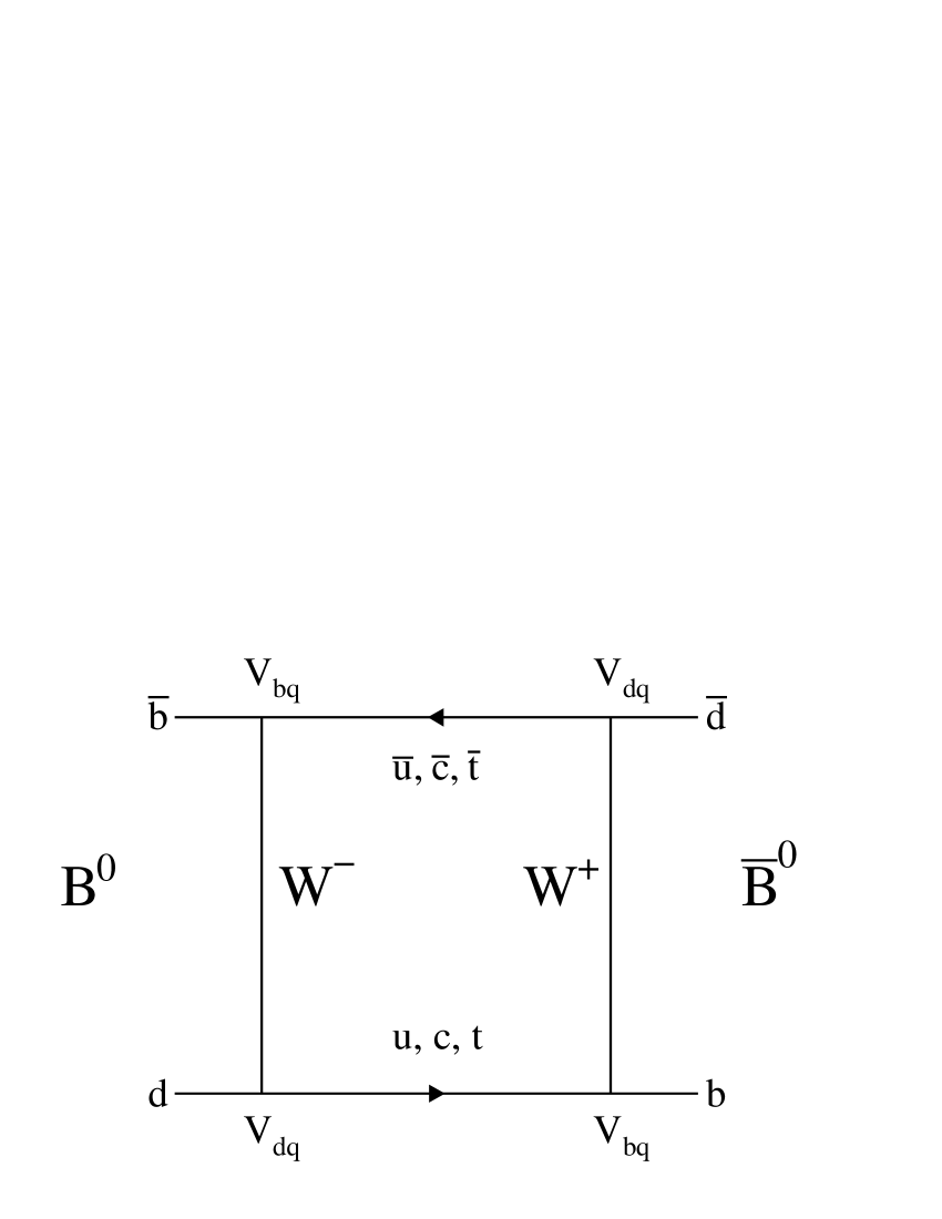
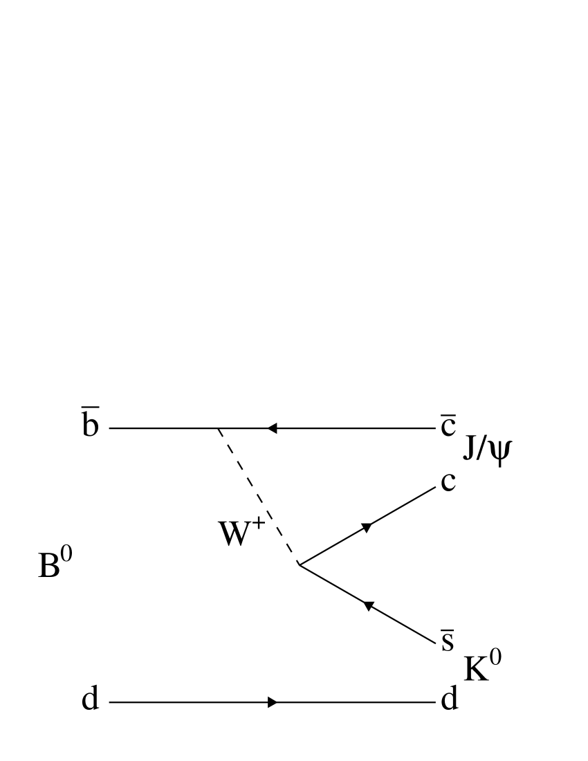
Figure 2: The (left) mixing and (right) tree contributions to Charmonium decays.

There are several calculations of the level of SM uncertainty on the measurement of $\sin 2\beta$ in $b\to c\overline{c}s$ decays which include theoretical and data driven phenomenological estimates of this uncertainty [14, 15, 16]. The data driven method uses $B^{0}\to J/\psi\pi^{0}$ to limit the SM uncertainties at a level of $10^{-2}$, and the theoretical calculations limit these uncertainties to be ${\cal O}(10^{-3})$ to ${\cal O}(10^{-4})$. BABAR found a signal for $CP$ violation in $B$ meson decay in 2001 [17] and this result was confirmed two weeks later by Belle [18]. The latest analyses from the $B$ factories provide the most precise test of CKM theory [19, 20]. These results are summarised in Table 2 where the BABAR result uses $B$ decays to $J/\psi K^{0}$, $\psi(2S)K^{0}_{S}$, $\chi_{1c}K^{0}_{S}$, $\eta_{c}K^{0}_{S}$, and $J/\psi K^{*0}$ to measure $\sin 2\beta$. Belle use $J/\psi K^{0}$, and $\psi(2S)K^{0}_{S}$ final states for their measurement.

Experiment $\sin 2\beta$ BABAR $0.691\pm 0.029\mathrm{(stat.)}\pm 0.014\mathrm{(syst.)}$ Belle $0.650\pm 0.029\mathrm{(stat.)}\pm 0.018\mathrm{(syst.)}$ World Average $0.671\pm 0.024$

Table 2: Experimental results for $\sin 2\beta$ from the $B$ factories.

When converting the measured value of $\sin 2\beta$ to a value of $\beta$ we obtain a four fold ambiguity on $\beta$. The four solutions for beta are $21.1^{\circ}$, $68.9^{\circ}$, $201.1^{\circ}$, and $248.9^{\circ}$. The two solutions $68.9^{\circ}$ and $248.9^{\circ}$ are disfavoured by $\cos 2\beta$ measurements from decays such as $B^{0}\to J/\psi K^{*}$ [21], $D^{*}D^{*}K_{S}^{0}$ [22] and $D^{*0}h^{0}$ [23]. The only solution for $\beta$ that is consistent with the Standard Model is $\beta=(21.1\pm 0.9)^{\circ}$. This result corresponds to the first test of the CKM mechanism as the apex of the unitarity triangle can be constrained using Eq. 5. In order to fully constrain the theory, we need a second measurement from one of the observables described below.

As can be seen from Table 2, the precision of the $\sin 2\beta$ result from the $B$ factories is still limited by statistics. This measurement will be refined by the next generation of experiments, including LHCb [24], SuperB [25] and SuperKEKB [26]. For example, the measurement of $\sin 2\beta$ with 75$\mathrm{ab}^{-1}$ from SuperB will be systematics limited and have a precision of $\pm 0.005$ [25].

3.1.2 The angle $\alpha$

The measurement of $\alpha$ is not as straight forward as $\beta$. All of the decay channels that are sensitive to $\alpha$ have potentially large contributions from loop amplitudes, in addition to the leading order tree and mixing contributions. Figure 3 shows these tree and loop contributions. In the absence of a loop contribution, the interference between tree and mixing amplitudes would result in $S=\sin(2\alpha)$. Here the weak phase measured is $\alpha=\pi-\beta-\gamma$ where $\beta$ comes from the $V_{\mathrm{td}}$ vertices of the mixing amplitudes, and $\gamma$ comes from the $V_{\mathrm{ub}}$ vertex of the tree amplitude. However, the loop contributions have a different weak phase to the tree contribution, so they ’pollute’ the measurement of $\alpha$. There are two schemes used in order to determine the loop pollution $\delta\alpha$: (i) use $SU(2)$ relations [28], and (ii) use $SU(3)$ relations [32] to constrain the effect of loop amplitudes on the extraction of $\alpha$ from measurements of $B$ meson decays to $h^{+}h^{-}$ final states, where $h=\pi,\rho$. The effect of loop amplitudes is $\delta\alpha=\alpha-\alpha_{\mathrm{eff}}$, where $\alpha_{\mathrm{eff}}$ is related to the measured $S$ and $C$ via $S=\sqrt{1-C^{2}}\sin(2\alpha_{\mathrm{eff}})$.

Figure 3: The tree (left) and gluonic loop (right) contributions to $B\to h^{+}h^{-}$ decays.

One can use $SU(2)$ isospin to relate the amplitudes of $B$ decays to $\pi\pi$ final states [28]. This results in two relations:

$$\frac{1}{\sqrt{2}}A^{+-}=A^{+0}-A^{00},\,\,\,\,\,\,\,\frac{1}{\sqrt{2}}\overline{A}^{+-}=\overline{A}^{-0}-\overline{A}^{00},$$

where $A^{ij}$ ($\overline{A}^{ij}$) are the amplitudes of $B$ ($\overline{B}$) decays to the final state with charge $ij$. These two relations correspond to triangles in a complex plane with a common base given by $|A^{+0}|=|\overline{A}^{-0}|$ neglecting electroweak loop contributions. There are three such relations for $\rho\rho$ decays, one for each of the transversity states (Section 5). The extraction of $\alpha$ from $\rho\pi$ decays is complicated by the fact that the final state is not a $CP$ eigenstate [29, 30]. A more detailed overview of the experimental methods used for $\pi\pi$, $\rho\rho$, and $\rho\pi$ decays is given in Ref. [31].

The experimental results for $B\to\pi\pi$ [34, 35], $B\to\rho\rho$ [36, 37, 38, 39, 41, 40], and $B\to\rho\pi$ [42, 43] decays can be combined together in order to constrain $\alpha$. This constraint is shown in Figure 4 for the $SU(2)$ approach. The solution compatible with the SM is $\alpha=(91\pm 8)^{\circ}$ [33] which provides a second reference point to test the CKM mechanism.

Beneke at al. proposed the use of $SU(3)$ to relate the loop component of $B^{+}\to\rho^{-}K^{*0}$ to the loop component of $B^{0}\to\rho^{+}\rho^{-}$ [32]. In order to do this, one has to measure the branching fractions and fractions of longitudinally polarized signal in both decay channels, as well as $S$ and $C$ for the longitudinal polarization of $B^{0}\to\rho^{+}\rho^{-}$. On doing this, BABAR finds that $\alpha=(89.8^{+7.0}_{-6.4})^{\circ}$, where the corresponding loop to tree ratio measured is $0.10^{+0.03}_{-0.04}$ [37].

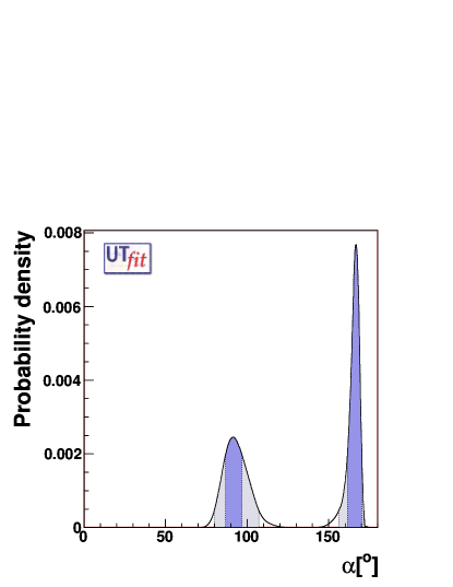
Figure 4: The constraint on $\alpha$ from an isospin analysis of $B\to hh$ decays. Constraints are made on the magnitude of the penguin to tree ratio for $B\to\pi\pi$ decays when making this plot. This figure is reproduced from UT fit [33]. The shaded regions correspond to the allowed solutions for $\alpha$.

The strongest constraint on $\alpha$ comes from the study of $B\to\rho\rho$ decays and this measurement is currently limited by statistics. The next generation of experiments will be able to refine our knowledge of $\alpha$: LHCb will be able to measure this to ${\cal O}(5^{\circ})$ [44] with 10$\mathrm{fb}^{-1}$ of data using $B\to\rho\pi$ decays, but will not be able to measure all of the necessary inputs for the $\pi\pi$ and $\rho\rho$ measurements. The SuperB experiment will be able to measure $\alpha$ to a level that will be limited by systematic and theoretical uncertainties: ${\cal O}(1-2^{\circ})$ [25] with a data sample of 75$\mathrm{ab}^{-1}$.

It is also possible to constrain $\alpha$ using $SU(3)$ based approaches for decays such as $B\to a_{1}\pi$, and $a_{1}\rho$. Even though these decays are experimentally challenging to measure, the time-dependent analysis of $B\to a_{1}\pi$ decays has been performed [45]. Additional experimental constraints, such as the branching fractions of $K_{1}\pi$ decays, are required to interpret those results as a measurement on $\alpha$. Only a branching fraction upper limit exists for $B^{0}\to a_{1}^{\pm}\rho^{\mp}$ [46].

3.1.3 The angle $\gamma$

There are several promising methods being pursued in order to constrain $\gamma$ or $\sin(2\beta+\gamma)$, however none of these provides as stringent a bound as those for $\beta$ and $\alpha$. Here I discuss three methods used to constrain $\gamma$: these are called Gronau-London-Wyler (GLW) [47], Attwood-Dunietz-Soni (ADS) [48] and Giri-Grossman-Soffer-Zupan (GGSZ) [49]. These three methods are theoretically clean, and use $B$ decays to $D^{(*)}K^{(*)}$ final states to measure $\gamma$.

The GLW method [47] uses $B^{+}\to D_{CP}^{0}X^{+}$ and $B^{+}\to\overline{D}_{CP}^{0}X^{+}$ where $X^{+}$ is a strangeness one state, and $D_{CP}^{0}$ is a $D^{0}$ decay to a $CP$ eigenstate (similarly for $\overline{D}_{CP}^{0}$) to extract $\gamma$. The $CP$-even eigenstates used are $D_{CP}^{0}\to h^{+}h^{-}$ where $h=\pi,K$, and the $CP$-odd eigenstates used are $D_{CP}^{0}\to K^{0}_{S}\pi^{0},K^{0}_{S}\omega$, and $K^{0}_{S}\phi$. The ratio of Cabibbo allowed to Cabibbo suppressed decays is given by the parameter $r_{B}$. The experimentally determined value is $r_{B}\sim 0.1$ which leads to a relatively a large uncertainty on $\gamma$ extracted using this method. A similar measurement has been performed using $D^{*0}_{CP}K$ decays, where $r_{B}^{*}$ is found to be $0.22\pm 0.09\pm 0.03$, and only weak constraints can be placed on $\gamma$ [52, 51].

The ADS method [48] uses the doubly Cabibbo suppressed decays $B^{+}\to D^{*0}K^{(*)\pm}$ where the interference between amplitudes with a $D$ and a $\overline{D}$ decaying into a $K^{+}\pi^{-}$ final state is sensitive to $\gamma$. As with the GLW method, the ADS method requires more statistics than are currently available in order to measure $\gamma$ [53, 54].

The GGSZ method [49] uses $B$ decays to $D^{(*)0}K^{(*)}$ final states where the $D^{(*)}$ subsequently decays to $K^{0}_{S}h^{+}h^{-}$ ($h=\pi,K$)to constrain $\gamma$. This method is self tagging either by the charge of the reconstructed $B^{\pm}$ meson, or by the charge of the reconstructed $K^{(*)}$ for neutral $B$ decays. One has to understand the $D$ Dalitz decay distribution to determine $\gamma$. Using this method Belle measure $\gamma=(76^{+12}_{-13}\pm 4\pm 9)^{\circ}$ [55] where the errors are statistical, systematic and model dependent. The corresponding BABAR measurement is $\gamma=(76^{+23}_{-24}\pm 5\pm 5)^{\circ}$ [56]. The difference in statistical uncertainties of these measurements comes from the fact that Belle measure a larger value of $r_{B}$ than BABAR.

Figure 5 shows the experimental constraint on $\gamma$ where the total precision on this angle is $20^{\circ}$ with a central value of $71^{\circ}$. The next generation of experiments will be able to refine our knowledge of $\gamma$: LHCb will be able to measure this to ${\cal O}(2^{\circ})$ [44] with 10$\mathrm{fb}^{-1}$ of data. The SuperB experiment will be able to measure $\gamma$ to ${\cal O}(1^{\circ})$ [25] with a data sample of 75$\mathrm{ab}^{-1}$.

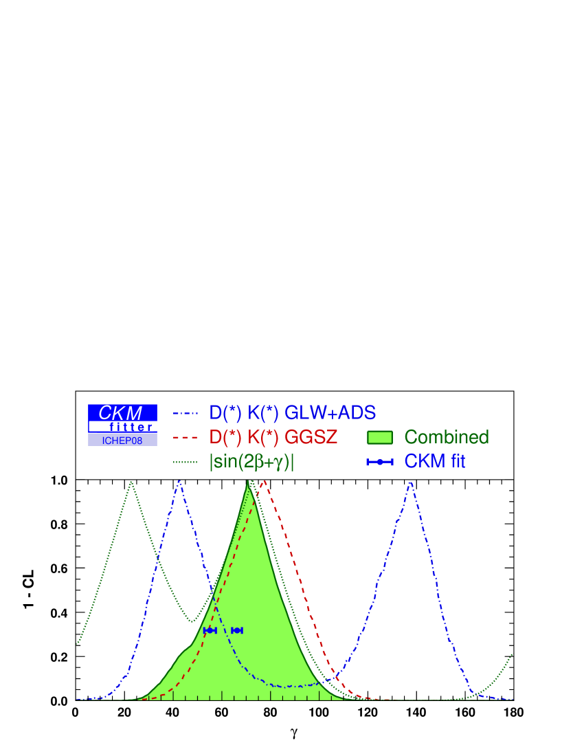
Figure 5: The experimental constraint on $\gamma$. This figure is from CKM Fitter [50].

3.1.4 Angle constraints on the CKM theory

The angle measurements described in the previous sections individually constrain CKM theory by restricting the allowed values of $\overline{\rho}$ and $\overline{\eta}$. The individual and combined constraints of these measurements are shown in Fig. 6. The angle constraints are consistent with CKM theory at the current level of precision. Combining the angle measurements: $\beta=(21.1\pm 0.9)^{\circ}$, $\alpha=(89.9^{+7.0}_{-6.4})^{\circ}$, and $\gamma=(71\pm 20)^{\circ}$, we obtain $\overline{\rho}=0.13\pm 0.04$ and $\overline{\eta}=0.34\pm 0.02$. The the precision on these constraints is dominated by our knowledge of $\alpha$ and $\beta$. CKM theory requires that $\alpha+\beta+\gamma=180^{\circ}$. The $B$ factory measurements give $\alpha+\beta+\gamma=(190\pm 21)^{\circ}$ where the precision of this test is limited by our knowledge of $\gamma$.

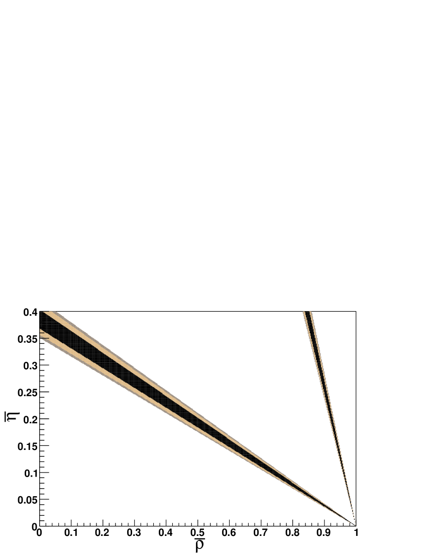
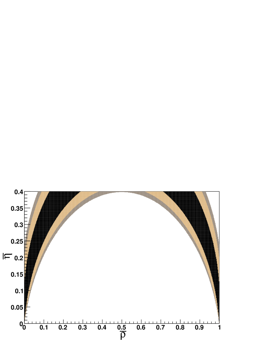
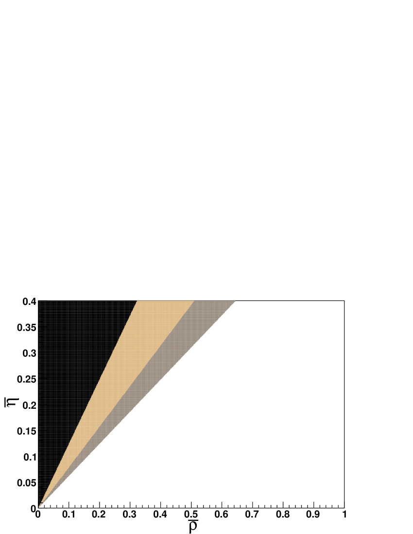
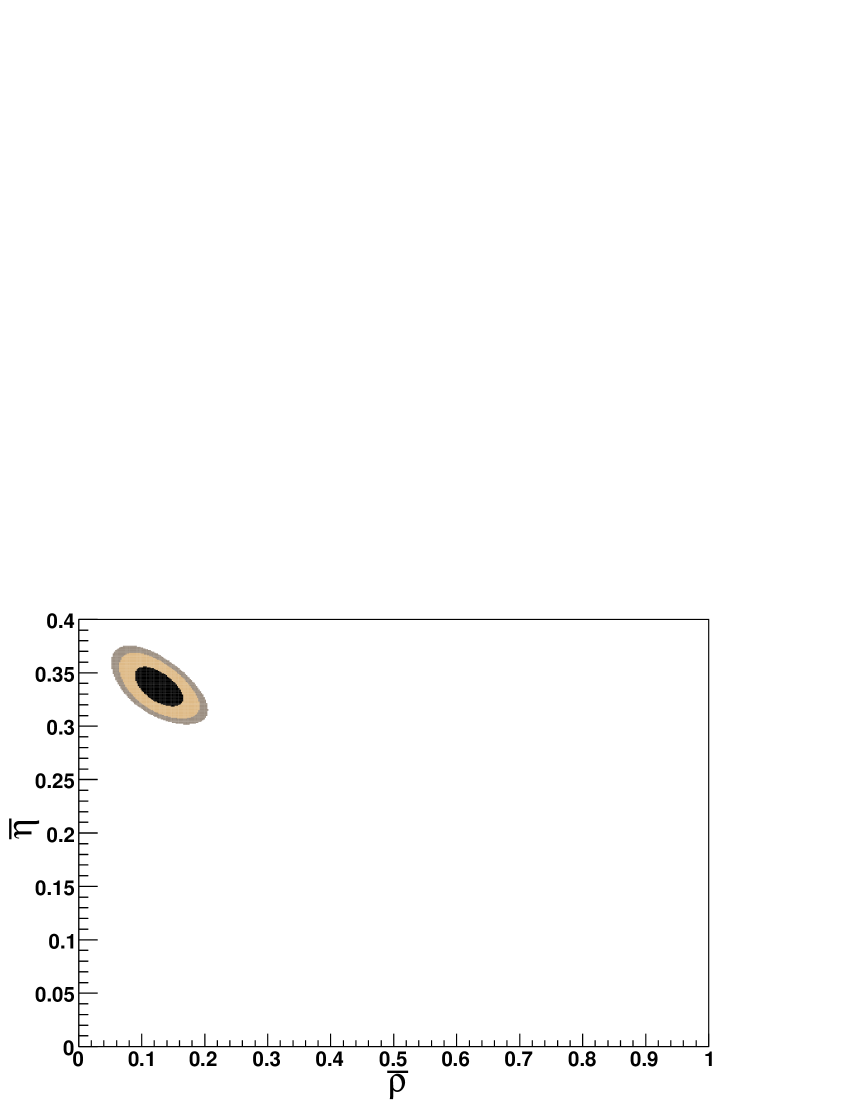
Figure 6: Angle constraints on $\overline{\rho}$ and $\overline{\eta}$ from (top left) $\beta$, (top right) $\alpha$, (bottom left) $\gamma$, and (bottom right) combined. The shaded contours show the 68% (black), 90% (light) and 95% (medium) confidence levels.

3.1.5 Direct $CP$ violation

Experiment $A_{CP}$ BABAR $-0.107\pm 0.016^{+0.006}_{-0.004}$ [61] Belle $-0.094\pm 0.018\pm 0.008$ [60] CDF $-0.086\pm 0.023\pm 0.009$ [62] CLEO $-0.04\pm 0.16\pm 0.02$ [63]

Table 3: Experimental results for $A_{CP}$, where the first error quoted is statistical and the second is systematic.

Direct $CP$ violation was established by the NA48 and KTeV experiments in 1999 [57, 58] through the measurement of a non-zero value of the parameter $\epsilon^{\prime}/\epsilon$. This phenomenon was confirmed 45 years after $CP$ violation was discovered in kaon decays. In contrast to this in $B$ meson decay direct $CP$ violation was observed only a few years after $CP$ violation was established. The first observation of direct $CP$ violation in $B$ decays was made via the measurement of a non-zero $A_{CP}$ in $B^{0}\to K^{\pm}\pi^{\mp}$ decays in 2007 by BABAR [59]. The following year Belle confirmed this result [60]. The latest results of this measurement are summarised in Table 3. It has been suggested that the difference in the direct $CP$ violation observed in $B^{0}\to K^{\pm}\pi^{\mp}$ and $B^{+}\to K^{+}\pi^{0}$ could be due to new physics (See Ref. [59] and references therein). A more plausible explanation is that the difference arises from final state interactions [64].

3.1.6 Searching for new physics

The $B$ factories have seen evidence for, or have observed indirect $CP$ violation in $B^{0}\to J/\psi K^{0}$, $B^{0}\to J/\psi\pi^{0}$, $B^{0}\to\psi(2S)K^{0}_{S}$, $B^{0}\to\eta_{1c}K^{0}_{S}$, $B^{0}\to\eta^{\prime}K^{0}$, $B^{0}\to f_{0}^{0}(980)K^{0}_{S}$, $B^{0}\to K^{+}K^{-}K^{0}$, $B^{0}\to D^{*+}D^{*-}$, and $B^{0}\to\pi^{+}\pi^{-}$. They have also seen evidence for or observed direct $CP$ violation in $B^{0}\to\pi^{+}\pi^{-}$, $B^{0}\to\eta K^{*0}$, $B^{0}\to\rho^{\pm}\pi^{\mp}$, $B^{0}\to K^{\pm}\pi^{\mp}$, $B^{\pm}\to\rho^{0}K^{\mp}$, $B\to D^{0}_{CP+}K$, $B\to D^{(*)0}K^{*}$. All of the measurements of $CP$ violating asymmetries to date are consistent with CKM theory. It is possible that there is more to $CP$ violation than the CKM theory and the rest of this section discusses one way to search for effects beyond CKM.

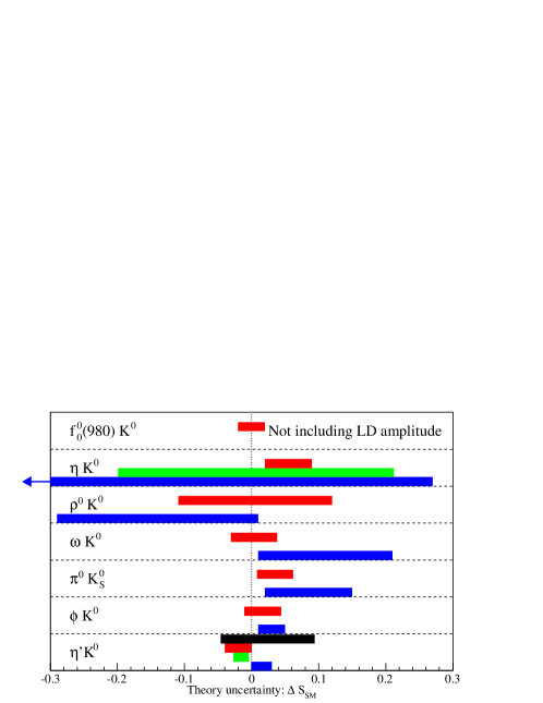
Figure 7: Theoretical estimates of $\Delta S_{\mathrm{SM}}$.

A large number of rare $B$ decays are sensitive to $\beta$ however as these measurements are not necessarily clean we call the phase measured $\beta_{\mathrm{eff}}$. These fall into two categories: those that are loop dominated; and those that have a loop and a tree contribution. The SM loop amplitude can be replaced by a corresponding amplitude with unknown heavy particles, for example the SUSY partners of the SM loop constituents, so the loops are sensitive to the presence of new physics. The consequence of this is that if there are new heavy particles that contribute to the loop, the SM calculated expectation for observables will differ from experimental measurements of the observables. $\sin 2\beta$ has been measured to an accuracy of $1^{\circ}$ using tree dominated $c\overline{c}s$ decays and this can be used as a reference point to test for deviations from the SM. If we measure $\sin 2\beta_{\mathrm{eff}}$ for a rare decay, then $\Delta S=\sin 2\beta_{\mathrm{eff}}-\sin 2\beta-\Delta S_{\mathrm{SM}}$ is zero in the absence of new physics. Here $\Delta S_{\mathrm{SM}}$ is a term that accounts for the effect of possible higher order SM contributions to a process that would lead to the measured $\sin 2\beta_{\mathrm{eff}}$ differing from the $c\overline{c}s$ measurement. Such effects include contributions from long distance scattering (LD), annihilation topologies and other often neglected terms. There has been considerable theoretical effort in recent years to try and constrain $\Delta S_{\mathrm{SM}}$ which is summarised in Figure 7. The figure is divided into decay modes, and each decay mode has up to four error bands drawn on it. These error bands come from (top to bottom) calculations by Beneke at al. [65], Williamson and Zupan [66], Cheng at al. [67], and Gronau at al. [68]. It is clear from this work that some of the decay modes are clean, and the SM expectation of $\sin 2\beta_{\mathrm{eff}}$ is essentially the same as the expectation for $\sin 2\beta$ from $c\overline{c}s$. However some modes have a significant contribution to $\Delta S$ from $\Delta S_{\mathrm{SM}}$. The experimental situation is shown in Figure 8 [69].

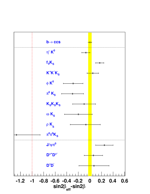
Figure 8: Measurements of $\sin 2\beta_{\mathrm{eff}}$-$\sin 2\beta$. The top part and vertical band show the reference measurement from $c\overline{c}s$ decays (See Sec. 3.1.1), the middle part shows measurements from $b\to s$ loop processes, and the part section shows measurements from $b\to d$ processes with loop and tree contributions. All results shown are averages of measurements from BABAR and Belle.

The most precisely determined $\sin 2\beta_{\mathrm{eff}}$ from a $b\to s$ loop process is that of $B^{0}\to\eta^{\prime}K^{0}$. This is also one of the theoretically cleanest channels, and is consistent with the SM expectation of $\Delta S=0$ at the current precision. In recent years it has been frequently noted that the average value of $\sin 2\beta_{\mathrm{eff}}-\sin 2\beta$ is less than zero with a significance of between two and three standard deviations. However as discussed above, it is not correct to compare the average of any set of processes unless the value of $\Delta S_{\mathrm{SM}}$ is the same for that set. If one wants to make a comparison at the percent level, it has to be done on a mode-by-mode basis, and to do that we need to build a next generation of experiments to record and analyse ${\cal{O}}(50-100)\mathrm{ab}^{-1}$ of data. The two proposed experiments SuperB and SuperKEKB will be able to make such measurements. If one compares the measured values of $\sin 2\beta_{\mathrm{eff}}-\sin 2\beta$ for the $b\to d$ processes which have a tree and a loop contribution it is clear that they are consistent with the SM expectation. At future $B$ factories it will be possible to extend this approach to making comparisons of the precision measurements of $\alpha$ and $\gamma$ from different decay channels.

3.2 Side measurements

This section discusses the measurements of $|V_{\mathrm{ub}}|$, $|V_{\mathrm{cb}}|$, and $|V_{\mathrm{td}}/V_{\mathrm{ts}}|$ in turn. All of these quantities are can be used to constrain the unitarity triangle. The measurements of $|V_{\mathrm{ub}}|$ and $|V_{\mathrm{cb}}|$ use the semi-leptonic decays $B\to X\ell\nu$ where $X=X_{u}$ or $X_{c}$ and it is possible to put constraints on $|V_{\mathrm{td}}/V_{\mathrm{ts}}|$ by measuring $B\to X_{d,s}\gamma$ decays.

3.2.1 Measuring $|V_{\mathrm{ub}}|$

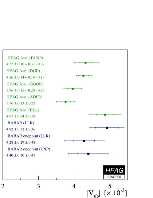
Figure 9: Constraints on $|V_{\mathrm{ub}}|$ compiled by HFAG [71].

The branching ratios of $B$ decays to $u\ell\nu$ semi-leptonic final states are proportional to $|V_{\mathrm{ub}}|$ for a limited region of phase space. In order to reduce backgrounds in these measurements, both $B$ mesons in the event are reconstructed using the so-called recoil method. This involves reconstructing the inclusive or exclusive $b\to u\ell\nu$ signal, as well as reconstructing everything else in the event into a fully reconstructed final state (i.e. one with no missing energy). If this is done correctly for a $B\overline{B}$ event, then the missing 4-momentum in the centre of mass will correspond to the 4-momentum of the undetected $\nu$ from the signal decay. The recoil method results in low signal efficiencies, typically a few percent, however most of the non-$B$ background will have been rejected from the selected sample of events and the signal sample is relatively clean. Once isolated, it is possible to measure the partial branching fraction of a decay as a function of a phase space variable, including the $q^{2}$ of the $\ell\nu$ in the final state, the invariant mass of the $X_{u}$, missing mass (corresponding to the neutrino), or energy of the lepton.

Given the partial branching fraction measurement, theoretical input is required in order to compute $|V_{\mathrm{ub}}|$. There are several schemes available to convert the partial branching fraction to a measurement of $|V_{\mathrm{ub}}|$ (ADFR, BLNP, BLL, DGE, GGOU, LLR, and LNP), and all of these schemes  [70] give compatible results [71]. Figure 9 shows the different values of $|V_{\mathrm{ub}}|$ extracted from the data for the different schemes where the LLR and LNP schemes use $B\to X_{u}\ell\nu$ decays normalised to $B\to X_{s}\gamma$ decays in order to determine $|V_{\mathrm{ub}}|$.

3.2.2 Measuring $|V_{\mathrm{cb}}|$

The recoil method discussed above is also used in order to isolate signals in the measurement of $|V_{\mathrm{cb}}|$. Only two decay channels are considered (i) $B\to D\ell^{+}\overline{\nu}$ and (ii) $B^{+}\to D^{*0}\ell^{+}\overline{\nu}$ where the partial branching fraction of these decays is proportional to $|V_{\mathrm{cb}}|$ up to some form factor.

The partial branching fraction of $B\to D\ell^{+}\overline{\nu}$ is proportional to $G^{2}|V_{\mathrm{cb}}|^{2}$, where $G$ is a form factor that depends on kinematic quantities. As the measurement is statistically limited, seven (nine) different $D^{0}$ ($D^{+}$) daughter decays into final states with neutral and charged pions and kaons are reconstructed. The results obtained using a combined fit to all data are $G(1)|V_{\mathrm{cb}}|=(43.0\pm 1.9\pm 1.4)\times 10^{-3}$, where $|V_{\mathrm{cb}}|=(39.8\pm 1.8\pm 1.3\pm 0.9)\times 10^{-3}$ [71] where this result is dominated by BABAR [72, 73]. Errors are statistical, systematic and from the form factor dependence. Figure 10 shows the distribution of $G(1)|V_{\mathrm{cb}}|$ versus $\rho^{2}$ obtained, where the form factor $G$ depends on the shape parameter $\rho^{2}$.

The partial branching fraction of $B^{+}\to D^{*0}\ell^{+}\overline{\nu}$ is proportional to $F^{2}|V_{\mathrm{cb}}|^{2}$, where $F$ is a form factor that depends on kinematic quantities. The measurement of $|V_{\mathrm{ub}}|$ using this mode is systematically limited, and as a result the only $D^{*0}$ daughter decay channel considered is to a $D^{0}\pi$ final state, where the $D$ meson subsequently decays to $K^{+}\pi^{-}$. The values of $F(1)|V_{\mathrm{cb}}|$ and the slope parameter $\rho^{2}$ are extracted from a three dimensional fit to data, where the discriminating variables in the fit are the mass difference between the reconstructed $D^{*}$ and $D$ meson masses $\Delta m$, the angle between the $B$ and the $Y=D^{*}\ell$ in the centre of mass $\theta_{BY}^{*}$ and an estimator for the dot product of the four velocities of the $B$ and the $D^{*}$. The results obtained are $F(1)|V_{\mathrm{cb}}|=(35.97\pm 0.53)\times 10^{-3}$ and $|V_{\mathrm{cb}}|=(38.7\pm 0.6\pm 0.9)\times 10^{-3}$, where the first uncertainty is experimental and the second is theoretical [71] where this result is dominated by Belle and BABAR [73, 74, 75, 76]. Figure 10 shows the distribution of $F(1)|V_{\mathrm{cb}}|$ versus $\rho^{2}$.

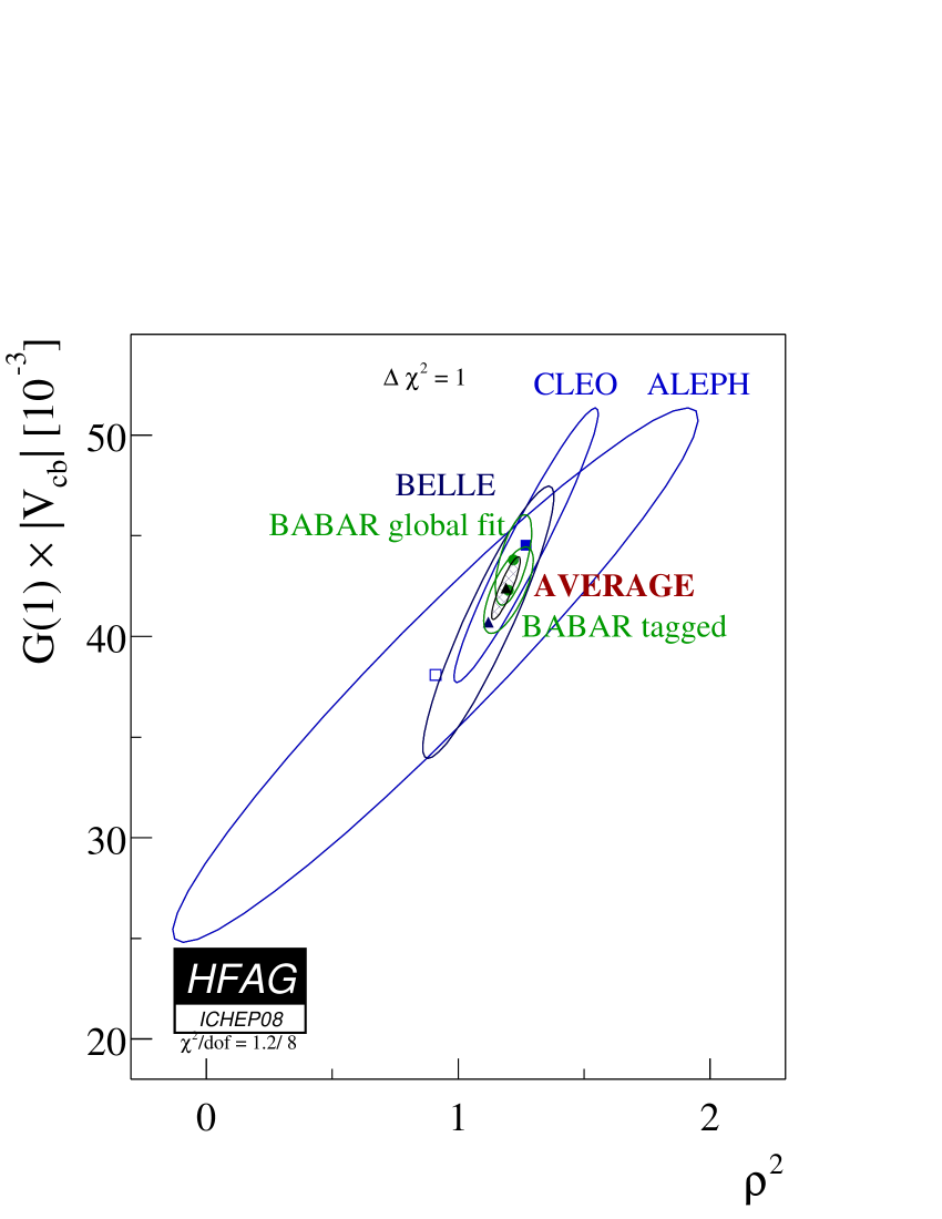
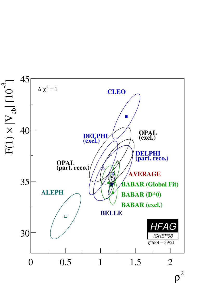
Figure 10: Measurements of (left) $G(1)|V_{\mathrm{cb}}|$ and (right) $F(1)|V_{\mathrm{cb}}|$ versus the slope $\rho^{2}$ obtained from $D^{(*)}\ell\overline{\nu}$ decays. These plots are from Ref. [71].

3.2.3 Measuring $|V_{\mathrm{td}}/V_{\mathrm{ts}}|$

It is possible to measure the ratio $|V_{\mathrm{td}}/V_{\mathrm{ts}}|$ using $B\to X_{d}\gamma$ and $B\to X_{s}\gamma$ decays as outlined by Ali, Asatrian and Greub [77]. The branching fractions of these processes depend on $|V_{\mathrm{td}}|$ and $|V_{\mathrm{ts}}|$, respectively. These are Flavour Changing Neutral Currents that are sensitive to new physics, where the leading order contributions are electroweak loop amplitudes. BABAR perform an inclusive analysis of $B\to X_{d}\gamma$ decays where $X_{d}$ is reconstructed from between two and four $\pi$ mesons, or a $\pi^{+}\eta$ final state, and extract a branching fraction in two regions of the invariant mass $m_{X}$ of $X_{d}$ [78]. Belle perform an exclusive analysis and reconstruct $X_{d}$ in $\rho$ and $\omega$ final states [79]. The branching fractions measured are summarised in Table 4.

Experiment	Region/mode	${\cal{B}}$ ($\times 10^{-6}$)
BABAR	$0.6<m_{X}<1.0$ $GeV/c^{2}$	$1.2\pm 0.5\pm 0.1$
BABAR	$1.0<m_{X}<1.8$ $GeV/c^{2}$	$2.7\pm 1.2\pm 0.4$
Belle	$B^{+}\to\rho^{+}\gamma$	$0.87^{+0.29}_{-0.27}\,{}^{+0.09}_{-0.11}$
Belle	$B^{0}\to\rho^{0}\gamma$	$0.78^{+0.17}_{-0.16}\,{}^{+0.09}_{-0.10}$
Belle	$B^{0}\to\omega\gamma$	$0.40^{+0.19}_{-0.17}\,{}^{+0.09}_{-0.10}$

Table 4: Branching fraction $({\cal{B}})$ measurements for $B\to X_{d}\gamma$. Inclusive measurements shown are from BABAR, and exclusive measurements shown are from Belle.

The constraint on $|V_{\mathrm{td}}/V_{\mathrm{ts}}|$ obtained using these measurements are $0.195^{+0.020}_{-0.019}{\rm(expt)}\pm 0.015{\rm(theory)}$ and $0.177\pm 0.043{\rm(expt)}\pm 0.001{\rm(theory)}$ from Belle and BABAR, respectively. The small theoretical uncertainty on the BABAR measurement is the result of the method used to determine $|V_{\mathrm{td}}/V_{\mathrm{ts}}|$ from data.

4 Tests of $CPT$

The combined symmetry of $C$, $P$ and $T$ otherwise written as $CPT$ is conserved in locally gauge invariant quantum field theory. The role of $CPT$ in our understanding of physics is described in more detail in Refs. [80, 81, 82, 83] and an observation of $CPT$ violation would be a sign of new physics. $CPT$ violation could be manifest in neutral meson mixing, so the $B$ factories are well suited to test this symmetry. The contribution to these proceedings by Nierst describes the phenomenon of neutral meson mixing in detail in terms of the complex parameters $p$ and $q$. It is possible to extend the formalism used by Nierst to allow for possible $CPT$ violation, and in doing so the heavy and light mass eigenstates of the $B^{0}$ meson $B_{\mathrm{H}}$ and $B_{\mathrm{L}}$ become

$$|B_{\mathrm{L,H}}\rangle=p\sqrt{1\mp z}|B^{0}\rangle\pm q\sqrt{1\pm z}|\overline{B}^{0}\rangle,$$

where $B^{0}$ and $\overline{B}^{0}$ are the strong eigenstates of the neutral $B$ meson. If we set $z=0$ we recover the $CPT$ conserving solution and if $CP$ and $CPT$ are conserved in mixing then $|q|^{2}+|p|^{2}=1$.

Two types of analysis have been performed by BABAR to test $CPT$. The first of these uses the $B_{\rm flav}$ sample that characterises the dilution and resolutions for the Charmonium $\sin 2\beta$ analysis discussed in Section 3.1 along with the Charmonium $CP$ eigenstates $B^{0}\to J/\psi K^{0}$, $\psi(2S)K^{0}_{S}$, and $\chi_{1c}K^{0}_{S}$ to extract $z$ [86]. This analysis also uses control samples of charged $B$ decays: $B^{+}\to\overline{D}^{(*)0}\pi^{+}$, $J/\psi K^{(*)+}$, $\psi(2S)K^{+}$, and $\chi_{1c}K^{+}$ to obtain

$$\left|\frac{q}{p}\right| = 1.029\pm 0.013\mathrm{(stat.)}\pm 0.011\mathrm{(syst.)},$$

$$(\mathrm{Re}\lambda_{\mathrm{CP}}/|\lambda_{\mathrm{CP}}|)\mathrm{Re}z = 0.014\pm 0.035\mathrm{(stat.)}\pm 0.034\mathrm{(syst.)},$$

$$\mathrm{Im}z = 0.038\pm 0.029\mathrm{(stat.)}\pm 0.025\mathrm{(syst.)},$$

which is compatible with no $CP$ violation in $B^{0}-\overline{B}^{0}$ mixing and $CPT$ conservation.

The second and more powerful type of analysis uses di-lepton events where both $B$ mesons in an event decay into an $X^{\mp}\ell^{\pm}\nu$ final state tests $CPT$. Di-lepton events can be grouped by lepton charge into three types: $++$, $+-$ and $--$ where the numbers of such events $N^{++}$, $N^{+-}$ and $N^{--}$ are related to $\Delta\Gamma$ and $z$ as a function of $\Delta t$ as described in Ref. [89]. Using these distributions we can construct two asymmetries: the first is a $T$/$CP$ asymmetry

$${\cal A}_{T/CP}=\frac{P(\overline{B}^{0}\to B^{0})-P(B^{0}\to\overline{B}^{0})}{P(\overline{B}^{0}\to B^{0})+P(B^{0}\to\overline{B}^{0})}=\frac{N^{++}-N^{--}}{N^{++}-N^{--}}=\frac{1-\left|\frac{q}{p}\right|^{4}}{1+\left|\frac{q}{p}\right|^{4}},$$

and the second is a $CPT$ asymmetry

$${\cal A}_{CPT}(\Delta t) = \frac{N^{+-}(\Delta t>0)-N^{+-}(\Delta t<0)}{N^{+-}(\Delta t>0)+N^{+-}(\Delta t<0)}\simeq 2\frac{\mathrm{Im}z\sin(\Delta m_{d}\Delta t)-\mathrm{Re}z\sinh\left(\frac{\Delta\Gamma\Delta t}{2}\right)}{\cosh\left(\frac{\Delta\Gamma\Delta t}{2}\right)+\cos(\Delta m_{d}\Delta t)},$$

where ${\cal A}_{CPT}(\Delta t)$ is sensitive to $\Delta\Gamma\times\mathrm{Re}z$. In the Standard Model ${\cal A}_{T/CP}\sim 10^{-3}$ and ${\cal A}_{CPT}=0$ [84, 85]. BABAR measure [87]

$$\left|\frac{q}{p}\right|-1 = (-0.8\pm 2.7\mathrm{(stat.)}\pm 1.9\mathrm{(syst.)})\times 10^{-3},$$

$$\mathrm{Im}z = (-13.9\pm 7.3\mathrm{(stat.)}\pm 3.2\mathrm{(syst.)})\times 10^{-3},$$

$$\Delta\Gamma\times\mathrm{Re}z = (-7.1\pm 3.9\mathrm{(stat.)}\pm 2.0\mathrm{(syst.)})\times 10^{-3},$$

which is compatible with no $CP$ violation in $B^{0}-\overline{B}^{0}$ mixing and $CPT$ conservation. It is possible to study variations as a function of sidereal time, where 1 sidereal day is approximately $0.99727$ solar days [88] where $z$ depends on the four momentum of the $B$ candidate. BABAR re-analysed their data to and find that it is consistent with $z=0$ at 2.8 standard deviations [89]. The constraint on $z$ is shown in Figure 11.

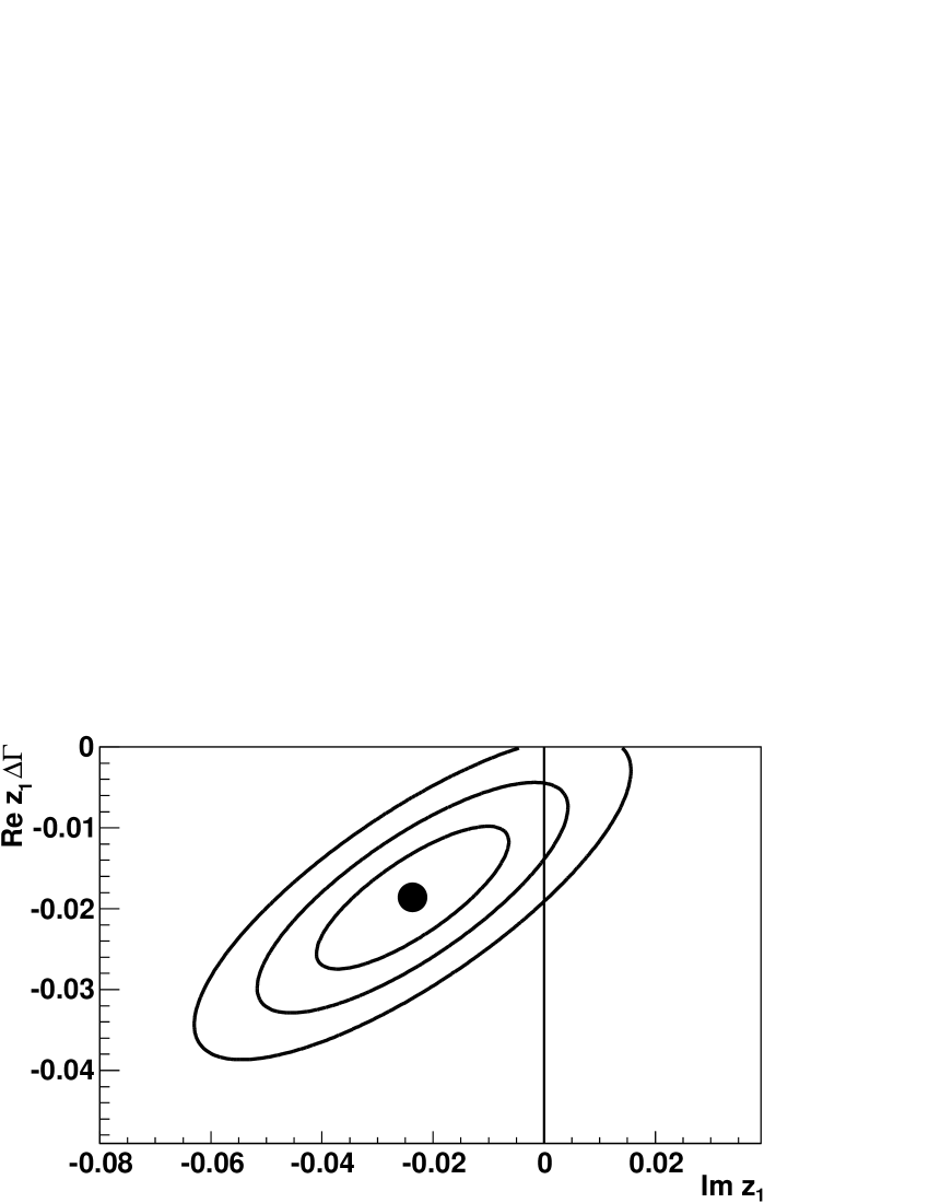
Figure 11: Constraints on the imaginary part of $z$ and $\Delta\Gamma\times\mathrm{Re}z$ using dilepton events at BABAR. This figure is reproduced from Ref. [89].

5 $B$ decays to spin one particles

Figure 12: A schematic of the decay of a $B$ meson via two $\rho$ mesons to a four pion final state. The $\rho$ meson final states are shown in their rest frames, and $\phi$ is the angle between the decay planes of the $\rho$ mesons.

Decays of $B$ mesons to final states with two vector ($J^{P}=1^{-}$) or axial-vector ($J^{P}=1^{+}$) particles have a number of interesting kinematic observables that can be used to test theoretical understanding of heavy flavour. The angular distribution of such a process where the spin one particles decay into two daughters is a function of three variables: $\phi$, $\theta_{1}$ and $\theta_{2}$, where $\phi$ is the angle between the decay planes of the spin one particles, and $\theta_{i}$ are the angles between the spin one particle decay daughter momentum and the direction opposite to that of the $B^{0}$ in the spin one particle rest frame. The $\theta_{i}$ are often referred to as helicity angles. Figure 12 illustrates these three angles for the decay $B^{0}\to\rho^{+}\rho^{-}$.

It is only possible to perform a full angular analysis if we have sufficient data to constrain the unknown observables. When we search for a rare decay it is normal to perform a simplified angular analysis in terms of the helicity angles, having first integrated over $\phi$. On doing this one obtains

$$\frac{d^{2}\Gamma}{\Gamma d\cos\theta_{1}d\cos\theta_{2}}=\frac{9}{4}\left[f_{\mathrm{L}}\cos^{2}\theta_{1}\cos^{2}\theta_{2}+\frac{1}{4}(1-f_{\mathrm{L}})\sin^{2}\theta_{1}\sin^{2}\theta_{2}\right]$$

where the parameter $f_{\mathrm{L}}$ is referred to as the fraction of longitudinally polarized events which is given by

$$\frac{\Gamma_{L}}{\Gamma}=\frac{|H_{0}|^{2}}{|H_{0}|^{2}+|H_{+1}|^{2}+|H_{-1}|^{2}}=f_{\mathrm{L}},$$

where the $H_{i}$ are helicity amplitudes. It is convenient to analyse the data using the transversity basis when performing time-dependent $CP$ studies where the transversity amplitudes are $A_{0}=H_{0}$, $A_{\perp}=(H_{+1}-H_{-1})/\sqrt{2}$ and $A_{||}=(H_{+1}+H_{-1})/\sqrt{2}$ [90]. $A_{0}$ and $A_{||}$ are $CP$ even and $A_{\perp}$ is $CP$ odd. Helicity suppression arguments lead to the expectation of the following hierarchy:

$$A_{0}:A_{||}:A_{\perp}\sim{\cal{O}}\left(1\right):{\cal{O}}\left(\frac{m_{R}}{m_{B}}\right):{\cal{O}}\left(\frac{m_{R}}{m_{B}}\right)^{2},$$

where $m_{R}$ is the mass of the spin one resonance and $m_{B}$ is the $B$ meson mass. This hierarchy predicts that $f_{\mathrm{L}}=1-m_{R}^{2}/m_{B}^{2}$ [91, 92, 93, 94]. The $B$ factories have measured the fraction of longitudinally polarized events in a number of different channels, the results of which are shown in Table 5.

Decay Mode	BABAR	Belle
$B^{0}\to\phi K^{*0}$  [95, 96]	$0.494\pm 0.34\pm 0.013$	$0.45\pm 0.05\pm 0.02$
$B^{+}\to\phi K^{*+}$  [97, 96]	$0.49\pm 0.05\pm 0.03$	$0.52\pm 0.08\pm 0.03$
$B^{0}\to\rho^{+}\rho^{-}$  [37, 41]	$0.992\pm 0.024^{+0.026}_{-0.013}$	$0.941^{+0.034}_{-0.040}\pm 0.030$
$B^{0}\to\rho^{0}\rho^{0}$  [38, 40]	$0.75^{+0.11}_{-0.14}\pm 0.05$	…
$B^{+}\to\rho^{0}\rho^{-}$  [36, 39]	$0.905\pm 0.042^{+0.023}_{-0.027}$	$0.95\pm 0.11\pm 0.02$
$B^{0}\to\omega K^{*0}$  [98]	…	$0.56\pm 0.29^{+0.18}_{-0.08}$
$B^{+}\to\omega\rho^{*+}$  [99]	$0.82\pm 0.11\pm 0.02$	…
$B^{0}\to K^{*0}\overline{K}^{*0}$  [100]	$0.80^{+0.10}_{-0.12}\pm 0.06$	…
$B^{0}\to\rho^{0}K^{*0}$  [101]	$0.57\pm 0.09\pm 0.08$	…
$B^{+}\to\rho^{0}K^{*+}$  [101]	$0.96^{+0.04}_{-0.15}\pm 0.05$	…
$B^{+}\to\rho^{+}K^{*0}$  [101, 102]	$0.52\pm 0.10\pm 0.04$	$0.43\pm 0.11^{+0.05}_{-0.02}$

Table 5: Experimental results for $f_{\mathrm{L}}$ from $B$ meson decays to two vector meson final states. The first uncertainty is statistical and the second is systematic.

It is clear that the helicity suppression argument works for a number of the decay modes studied. These are all tree dominated processes such as $B\to\rho^{+}\rho^{-}$. It is also clear that there are several decay modes that do not behave in the same way. The most precisely measured channel that disagrees with the helicity suppression argument is $B^{0}\to\phi K^{*0}$, where $f_{\mathrm{L}}\sim 0.5$. This discrepancy is often called the ‘polarization puzzle’ in the literature. Several papers for example Ref. [92] have highlighted the possibility that new physics could be the source of the difference, however final state interactions or refined calculations could also account for the difference. The decay modes that do not follow the naive helicity suppression argument are all loop dominated. In addition to studying $B$ decays to final states with two vector particles, it is possible to study vector axial-vector and two axial-vector final states. Measurements of these decays could help refine our understanding of the source of the polarization puzzle. There are a number of rare decays that have suppressed standard model topologies, for example $B\to\phi\phi$ and $B\to\phi\rho$. Experimental limits on these decays are at the level of a few $10^{-7}$ [103]. These decays could be significantly enhanced by new physics, and Gronau and Rosner recently suggested that $\phi-\omega$ mixing could result in a significant enhancement of the $B\to\phi\rho^{+}$ decay [104].

6 Summary

The $B$ factories have produced a large number of results in many areas of flavour physics. The ability of the $B$ factories to quickly crosscheck each others results has been extremely beneficial to the development of experimental measurements and techniques over the past decade. Only a small number of these results have been discussed here: those pertaining to testing the unitarity triangle, $CPT$, and $B$ decays to final states with two spin one particles. These results are consistent with the CKM theory for $CP$ violation in the Standard Model. There are a number of measurements sensitive to new physics contributions that can be made at future experiments such as SuperB in Italy and Super KEK-B in Japan [25, 26]. Such precision tests of flavour physics could be used to elucidate the flavour structure beyond the Standard Model.

7 Acknowledgments

I wish to thank the organizers of this summer school for their hospitality and for giving me the opportunity to discuss the work described here. The $B$ factories have been phenomenally successful and without the collective efforts of both the BABAR and Belle collaborations and the corresponding wealth of theoretical work over the past 45 years I would not have been in a position to talk on such a vibrant area of research. This work has been funded in part by the STFC (United Kingdom) and by the U.S. Department of Energy under contract number DE-AC02-76SF00515.

References

- [1] J.H. Christenson, J.W. Cronin, V.L. Fitch, and R. Turlay, Phys. Rev. Lett. 13 138-140 (1964).
- [2] A. D. Sakharov, Pis’ma Zh. Eksp. Teor. Fiz. 5 32 (1967) [JETP Lett. 5 24 (1967)].
- [3] N. Cabibbo, Phys. Rev. Lett. 10 531 (1963).
- [4] M. Kobayashi and T. Maskawa, Prog. Theor. Phys 49 652 (1973).
- [5] I. Bigi and A. Sanda, Nucl. Phys. B193 85 (1981).
- [6] P. Oddone, Detector Considerations, Workshop on Conceptual Design of a Test Linear Collider: Possibilities for a B Anti-B Factory, Los Angeles, California, pp 423-446 (1987).
- [7] J. Dorfan, B-Factory Symposium, Stanford, October 2008.
- [8] BABAR Collaboration, Nucl. Instrum. Meth. Phys. Res., Sec. A 479 1 (2002).
- [9] PEP-II Conceptual Design Report, SLAC-R-418 (1993).
- [10] Belle Collaboration, Nucl. Instrum. Meth. Phys. Res., Sec. A 479 117 (2002).
- [11] KEKB B-factory Design Report, KEK Report 95-7 (1995).
- [12] BABAR Collaboration, Nucl. Instrum. Meth. Phys. Res., Sec. A 479, 1 (2002).
- [13] C. Amsler at al.., Phys. Lett. B 667 1 (2008).
- [14] H. Li and S. Mishima, JHEP 0703 009 (2007).
- [15] H. Boos, J. Reuter, and T. Mannel, Phys. Rev. D 70, 036006 (2006).
- [16] M. Ciuchini, M. Pierini, and L. Silvestrini, Phys. Rev. Lett. 95, 221804 (2005).
- [17] BABAR Collaboration, Phys. Rev. Lett. 87 091801 (2001).
- [18] Belle Collaboration, Phys. Rev. Lett. 87 091802 (2001).
- [19] BABAR Collaboration, SLAC-PUB-13324; BABAR Collaboration, Phys. Rev. Lett. 99, 171803.
- [20] Belle Collaboration, Phys. Rev. Lett. 98, 031802 (2007); Belle Collaboration, Phys. Rev. D 77, 091103 (2008).
- [21] BABAR Collaboration, Phys. Rev. D 71 032005 (2005); Belle Collaboration, Phys. Rev. Lett. 95 091601 (2005).
- [22] BABAR Collaboration, Phys. Rev. D 71 032005 (2005); Belle Collaboration, Phys. Rev. Lett. 95 091601 (2005).
- [23] BABAR Collaboration, Phys. Rev. Lett. 99 081801 (2007).
- [24] LHCb: http://lhcb.web.cern.ch/lhcb/.
- [25] SuperB: Conceptual Design Report, arXiv:0709.0451; Valencia Physics Workshop, arXiv:0810.1312. http://www.pi.infn.it/SuperB/.
- [26] Super KEK-B: http://superb.kek.jp/.
- [27] M. Shifman, ITEP Lectures in Particle Physics and Field Theory. 1 pp v-xi (1999); e-Print: hep-ph/9510397.
- [28] M. Gronau and D. London, Phys. Rev. Lett. 65, 3381 (1990).
- [29] H. Lipkin at al., Phys. Rev. D 44, 1454 (1991).
- [30] A. Snyder and H. Quinn, Phys. Rev. D 48, 2139 (1993); H. Quinn and J. Silva, Phys. Rev. D 62, 054002 (2000).
- [31] A. Bevan, Mod. Phys. Lett. A21 305-318 (2006).
- [32] M. Beneke at al., Phys. Lett. B 638 68 (2006).
- [33] UTfit Collaboration, http://www.utfit.org/.
- [34] Belle Collaboration, Phys. Rev. Lett. 98, 211801 (2007).
- [35] BABAR Collaboration, arXiv:0807.4226.
- [36] BABAR Collaboration, Phys. Rev. Lett. 97, 261801 (2006).
- [37] BABAR Collaboration, Phys. Rev. D 76, 052007 (2007); BABAR Collaboration, Phys. Rev. Lett. 93 231801 (2004).
- [38] BABAR Collaboration, arXiv:0807.4977.
- [39] Belle Collaboration, Phys. Rev. Lett. 91, 221801 (2003).
- [40] Belle Collaboration, arXiv:0708.2006.
- [41] Belle Collaboration, Phys. Rev. D 76, 011104 (2007).
- [42] BABAR Collaboration, Phys. Rev. D 76 012004 (2007).
- [43] Belle Collaboration, Phys. Rev. D 77 072001 (2008).
- [44] T. Nakada, Acta Phys. Polon. B38 299 (2007).
- [45] BABAR Collaboration, Phys. Rev. Lett. 98, 181803 (2007).
- [46] BABAR Collaboration, Phys. Rev. D 74 031104 (2006).
- [47] M. Gronau, D. London, and D. Wyler, Phys. Lett. B 253 483 (1991).
- [48] M. Attwood, I. Dunietz, and A. Soni, Phys. Rev. Lett. 78 3257 (1997).
- [49] A. Giri, Y. Grossman, A. Soffer, and J. Zupan, Phys. Rev. D 68 054018 (2003).
- [50] CKMfitter Group, Eur. Phys. J. C41 1-131 (2005), updates available at http://ckmfitter.in2p3.fr.
- [51] Belle Collaboration, Phys. Rev. D 73, 051106 (2006).
- [52] BABAR Collaboration, Phys. Rev. D 72, 071103 (2005); BABAR Collaboration, Phys. Rev. D 77, 111102 (2008); BABAR Collaboration, arXiv:0807.2408.
- [53] Belle Collaboration, Phys. Rev. D 78 071901 (2008).
- [54] BABAR Collaboration, Phys. Rev. D 72, 032004 (2005); BABAR Collaboration, Phys. Rev. D 72, 071104 (2005); BABAR Collaboration, Phys. Rev. D 76, 111101 (2007).
- [55] Belle Collaboration, arXiv:0803.3375.
- [56] BABAR Collaboration, Phys. Rev. D 78 034023 (2008).
- [57] V. Fanti at al., Phys. Lett. B 465 335 (1999).
- [58] A. Alavi-Harati at al., Phys. Rev. Lett. 83 22 (1999).
- [59] BABAR Collaboration, Phys. Rev. Lett. 99 021603 (2007).
- [60] Belle Collaboration, Nature 452 332 (2008).
- [61] BABAR Collaboration, arXiv:0807.4226.
- [62] CDF Collaboration, hep-ex/0612018.
- [63] CLEO Collaboration, Phys. Rev. Lett. 85 525 (2000).
- [64] C. K. Chua, Phys. Rev. D 78 076002 (2008).
- [65] M. Beneke at al., Phys. Lett. B620 143 (2005).
- [66] A. Williamson and J. Zupan, Phys. Rev. D 74 014003 (2006).
- [67] H.Y.Cheng at al., Phys. Rev. D 72 014006 (2005).
- [68] M. Gronau at al., Phys. Rev. D 74 093003 (2006).
- [69] Belle Collaboration, Phys. Rev. D 77, 071101 (2008); BABAR Collaboration, Phys. Rev. Lett. 101, 021801 (2008); Belle Collaboration, Phys. Rev. Lett. 98, 221802 (2007); Belle Collaboration, Phys. Rev. Lett. 98, 031802 (2007); BABAR Collaboration, arXiv:0809.1174; BABAR Collaboration, Phys. Rev. Lett. 99, 161802 (2007); BABAR Collaboration, Phys. Rev. D 76, 091101 (2007); BABAR Collaboration, arXiv:0708.2097; Belle Collaboration, Phys. Rev. D 76, 091103 (2007); BABAR Collaboration, Phys. Rev. Lett. 99, 161802 (2007); Belle Collaboration, arXiv:0708.1845; BABAR Collaboration, Phys. Rev. D 76, 071101 (2007); BABAR Collaboration, Phys. Rev. Lett. 99, 161802 (2007).
- [70] B. Lange at al., Phys. Rev. D 72 073006 (2005); J. R. Anderson and E. Gardi, JHEP 0601: 097 (2006); E. Gardi arXiv:0806.4524; P. Gambino at al., JHEP 0710 058 (2007); U. Aglietti at al., arXiv:0711.0860; C. W. Bauer at al., Phys. Rev. D 64 113004 (2001); A. Leibovich at al., Phys.Rev. D61 (2000) 053006; B. Lange at al., JHEP 0510 084 (2005).
- [71] HFAG Group, arXiv:0704.3575, partial update online at http://www.slac.stanford.edu/xorg/hfag.
- [72] BABAR Collaboration, arXiv:0807.4978.
- [73] BABAR Collaboration, arXiv:0809.0828.
- [74] Belle Collaboration, Phys. Lett. B 526, p247 (2002).
- [75] BABAR Collaboration, Phys. Rev. Lett. 100 231803 (2008).
- [76] BABAR Collaboration, Phys. Rev. D 77 032002 (2008).
- [77] A. Ali at al., Phys. Lett. B 429 87 (1998).
- [78] BABAR Collaboration, arXiv:0708.3702.
- [79] Belle Collaboration, Phys. Rev. Lett. 95 241801 (2005).
- [80] G. Lders, Mat. Fys. Medd. 28 5 (1954).
- [81] R. Jost, Helv. Phys. Acta 30 409 (1957).
- [82] W. Pauli, Nuovo Cimento 6 204 (1957).
- [83] F. Dyson, Phys. Rev. 110 579 (1958).
- [84] M. Beneke at al., Phys. Lett. B 576 173 (2003).
- [85] M. Ciuchini at al., JHEP 0308 031 (2003).
- [86] BABAR Collaboration, Phys. Rev. D 70 012007 (2004).
- [87] BABAR Collaboration, Phys. Rev. Lett. 96 251802 (2006).
- [88] V.A. Kostelecky, Phys. Rev. Lett. 80 1818 (1998).
- [89] BABAR Collaboration, Phys. Rev. Lett. 100 131802 (2008).
- [90] I. Dunietz at al., Phys. Rev. D 43 2193 (1991).
- [91] A. Ali at al., Phys. Rev. D 58 094009 (1998).
- [92] A. Kagan, Phys. Lett. B 601 151-163 (2004).
- [93] G. Kramer and W. Palmer, Phys. Rev. D 45 193 (1992).
- [94] M. Suzuki, Phys. Rev. D 66 054018 (2002).
- [95] BABAR Collaboration, arXiv:0808.3586.
- [96] Belle Collaboration, Phys. Rev. Lett. 94 221804 (2005).
- [97] BABAR Collaboration, Phys. Rev. Lett. 99 201802 (2007).
- [98] Belle Collaboration, arXiv:0807.4271.
- [99] BABAR Collaboration, Phys. Rev. D 74 051102 (2006).
- [100] BABAR Collaboration, Phys. Rev. Lett. 100 081801 (2008).
- [101] BABAR Collaboration, Phys. Rev. Lett. 97 201801 (2006).
- [102] Belle Collaboration, Phys. Rev. Lett. 95 141801 (2005).
- [103] BABAR Collaboration, arXiv:0807.3935.
- [104] M. Gronau and J. Rosner, arXiv:0806.3584.