Temporal and Spatial Dependence of Quantum Entanglement
from a Field Theory Perspective

Abstract

We consider the entanglement dynamics between two Unruh-DeWitt detectors at rest separated at a distance $d$. This simple model when analyzed properly in quantum field theory shows many interesting facets and helps to dispel some misunderstandings of entanglement dynamics. We find that there is spatial dependence of quantum entanglement in the stable regime due to the phase difference of vacuum fluctuations the two detectors experience, together with the interference of the mutual influences from the backreaction of one detector on the other. When two initially entangled detectors are still outside each other’s light cone, the entanglement oscillates in time with an amplitude dependent on spatial separation $d$. When the two detectors begin to have causal contact, an interference pattern of the relative degree of entanglement (compared to those at spatial infinity) develops a parametric dependence on $d$. The detectors separated at those $d$ with a stronger relative degree of entanglement enjoy longer disentanglement times. In the cases with weak coupling and large separation, the detectors always disentangle at late times. For sufficiently small $d$, the two detectors can have residual entanglement even if they initially were in a separable state, while for $d$ a little larger, there could be transient entanglement created by mutual influences. However, we see no evidence of entanglement creation outside the light cone for initially separable states.

I Introduction

Recently we have studied the disentanglement process between two spatially separated Unruh-DeWitt (UD) detectors (pointlike objects with internal degrees of freedom) or atoms, described by harmonic oscillators, moving in a common quantum field: One at rest (Alice), the other uniformly accelerating (Rob) LCH08 . These two detectors are set to be entangled initially, while the initial state of the field is the Minkowski vacuum. In all cases studied in LCH08 , we obtain finite-time disentanglement (called “sudden death” of quantum entanglement YE04 ), which are coordinate dependent while the entanglement between the two detectors at two spacetime points is independent of the choice of time slice connecting these two events. Around the moment of complete disentanglement there may be some short-time revival of entanglement within a few periods of oscillations intrinsic to the detectors. In the strong-coupling regime, the strong impact of vacuum fluctuations experienced locally by each detector destroys their entanglement right after the coupling is switched on.

In the above situation we find in LCH08 the event horizon for the uniformly accelerated detector (Rob) cuts off the higher-order corrections of mutual influences, and the asymmetric motions of Alice and Rob obscure the dependence of the entanglement on the spatial separation between them. To understand better how entanglement dynamics depends on the spatial separation between two quantum objects, in this paper we consider the entanglement between two detectors at rest separated at a distance $d$, possibly the simplest setup one could imagine. This will serve as a concrete model for us to investigate and explicate many subtle points and some essential misconceptions related to quantum entanglement elicited by the classic paper of Einstein-Podolsky-Rosen (EPR) EPR .

I.1 Entanglement at spacelike separation: quantum nonlocality?

One such misconception (or misnomer, for those who understand the physics but connive to the use of the terminology) is “quantum nonlocality” used broadly and often too loosely in certain communities . Some authors think that quantum entanglement entails some kind of “spooky action at a distance” between two spacelike separated quantum entities (qubits, for example), and may even extrapolate this to mean “quantum nonlocality.” The phrase “spooky action at a distance” when traced to the source BE47 refers to the dependence of “what really exists at one event” on what kind of measurement is carried out at the other, namely, the consequence of measuring one part of an entangled pair. Without bringing in quantum measurement, one cannot explore fully the existence or consequences of “spooky action at a distance” but one could still talk about quantum entanglement between two spacelike separated qubits or detectors. This is the main theme of our present investigation. We show in a simple and generic model with calculations based on quantum field theory (QFT) that nontrivial dynamics of entanglement outside the light cone does exist.

Another misconception is that entanglement set up between two localized quantum entities is independent of their spatial separation. This is false for open systems interacting with an environment . This has already been shown in two earlier investigations of the authors ASH06 ; LCH08 and will be again in this paper.

A remark on nonlocality, or lack thereof, in QFT is in place here. QFT is often regarded as “local” in the sense that interactions of the fields take place at the same spacetime point , e.g., for a bosonic field $\phi(x)$, a local theory has no coupling of $\phi(x)$ and $\phi(y)$ at different spacetime points $x$ and $y$. It follows that the vacuum expectation value of the commutator $\left<\right.[\phi(x),\phi(y)]\left.\right>$ vanishes for all $y$ outside the light cone of $x$, which is what causality entails. Nevertheless, the Hadamard function $\left<\right.\{\phi(x),\phi(y)\}\left.\right>$ is nonvanishing in general, no matter $x-y$ is spacelike or timelike. In physical terms the Hadamard function can be related to quantum noise in a stochastic treatment of QFT HPZ . In this restricted sense one could say that QFT has certain nonlocal features. Of course it is well known that in QFT processes occurring at spacelike separated events such as virtual particle exchange are allowed.

I.2 Issues addressed here

With a careful and thorough analysis of this problem we are able to address the following issues:

1) Spatial separation between two detectors.–Ficek and Tanas FicTan06 as well as Anastopoulos, Shresta, and Hu (ASH) ASH06 studied the problem of two spatially separated qubits interacting with a common electromagnetic field. The former authors while invoking the Born and Markov approximations find the appearance of dark periods and revivals. ASH treat the non-Markovian behavior without these approximations and find a different behavior at short distances. In particular, for weak coupling, they obtain analytic expressions for the dynamics of entanglement at a range of spatial separation between the two qubits, which cannot be obtained when the Born-Markov approximation is imposed. A model with two detectors at rest in a quantum field at finite temperature in (1+1)-dimensional spacetime has been considered by Shiokawa in Tom08 , where some dependence of the early-time entanglement dynamics on spatial separation can also be observed.

In LCH08 we did not see any simple proportionality between the initial separation of Alice and Rob’s detectors and the degree of entanglement: The larger the separation, the weaker the entanglement at some moments, but stronger at others. We wonder if this unclear pattern arises because the spatial separation of the two detectors in LCH08 changes in time and also in coordinate. In our present problem the spatial separation between the two detectors is well defined and remains constant in Minkowski time, so the dependence of entanglement on the spatial separation should be much clearer and distinctly identifiable.

2) Stronger mutual influences.–Among the cases we considered in LCH08 , the largest correction from the mutual influences is still under $2\%$ of the total while we have only the first and the second-order corrections from the mutual influences. There the difficulty for making progress is due to the complicated multidimensional integrations in computing the back-and-forth propagations of the backreactions sourced from the two detectors moving in different ways. Here, for the case with both detectors at rest, the integration is simpler and in some regimes we can include stronger and more higher-order corrections of the mutual influences on the evolution of quantum entanglement.

3) Creation of entanglement and residual entanglement.–In addition to finite-time disentanglement and the revival of quantum entanglement for two detectors initially entangled, which have been observed in LCH08 for a particular initial state, we expect to see other kinds of entanglement dynamics with various initial states and how it varies with spatial separations. Amongst the most interesting behavior we found the creation of entanglement from an initially separated state LHMC08 and the persistence of residual entanglement at late times for two close-by detectors PR07 .

I.3 Summary of our findings

When the mutual influences are sufficiently strong (under strong coupling or small separation), the fluctuations of the detectors with low natural frequency will accumulate, then get unstable and blow up. As the separation approaches a merge distance (quantified later), only for detectors with high enough natural frequencies will the fluctuations not diverge eventually but acting more and more like those in the two harmonic oscillator (2HO) quantum Brownian motion (QBM) models CYH07 ; PR07 (where the two HOs occupy the same spatial location) with renormalized frequencies.

If the duration of interaction is so short that each detector is still outside the light cone of the other detector, namely, before the first mutual influence reaches one another, the entanglement oscillates in time with an amplitude dependent on spatial separation: At some moments the larger the separation the weaker the entanglement, but at other moments, the stronger the entanglement. While such a behavior is affected by correlations of vacuum fluctuations locally experienced by the two detectors without causal contact, there is no evidence for entanglement generation outside the light cone suggested by Franson in Ref. Franson .

For an initially entangled pair of detectors, when one gets inside the light cone of the other, certain interference patterns develop: At distances where the interference is constructive the disentanglement times are longer than those at other distances. This behavior is more distinct when the mutual influences are negligible. For the detectors separable initially, entanglement can be generated by mutual influences if they are put close enough to each other.

At late times, under proper conditions, the detectors will be entangled if the separation is sufficiently small, and separable if the separation is greater than a specific finite distance. The late-time behavior of the detectors is governed by vacuum fluctuations of the field and independent of the initial state of the detectors.

Since the vacuum can be seen as the simplest medium that the two detectors immersed in, we expect that the intuitions acquired here will be useful in understanding quantum entanglement in atomic and condensed matter systems (upon replacing the field in vacuum by those in the medium). To this extent our results indicate that the dependence of quantum entanglement on spatial separation of qubits could enter in quantum gate operations (see ASH06 for comments on possible experimental tests of this effect in cavity ions), circuit layout, as well as having an effect on cluster states instrumental to measurement-based quantum computing.

I.4 Outline of this paper

This paper is organized as follows. In Sec. II we describe our model and the setup. In Sec. III the evolution of the operators is calculated, then the instability for detectors with low natural frequency is described in Sec. IV. We derive the zeroth-order results in Sec. V, and the late-time results in Sec. VI. Examples with different spatial separations of detectors in the weak-coupling limit are given in Sec. VII. We conclude with some discussions in Sec. VIII. A late-time analysis on the mode functions is performed in Appendix A, while an early-time analysis of the entanglement dynamics in the weak-coupling limit is given in Appendix B.

II The model

Let us consider the Unruh-DeWitt detector theory in (3+1)-dimensional Minkowski space described by the action LCH08 ; LH2005

$$S = -\int d^{4}x{1\over 2}\partial_{\mu}\Phi\partial^{\mu}\Phi+\sum_{j=A,B}\left\{\int d\tau_{j}{1\over 2}\left[\left(\partial_{\tau_{j}}Q_{j}\right)^{2}-\Omega_{0}^{2}Q_{j}^{2}\right]+\lambda_{0}\int d^{4}x\Phi(x)\int d\tau_{j}Q_{j}(\tau_{j})\delta^{4}\left(x^{\mu}-z_{j}^{\mu}(\tau_{j})\right)\right\},$$ (1)

where the scalar field $\Phi$ is assumed to be massless, and $\lambda_{0}$ is the coupling constant. $Q_{A}$ and $Q_{B}$ are the internal degrees of freedom of the two detectors, assumed to be two identical harmonic oscillators with mass $m_{0}=1$, bare natural frequency $\Omega_{0}$, and the same local time resolution so their cutoffs in two-point functions LH2005 are the same. The left detector is at rest along the world line $z_{A}^{\mu}(t)=(t,-d/2,0,0)$ and the right detector is sitting along $z_{B}^{\mu}(t)=(t,d/2,0,0)$. The proper times for $Q_{A}$ and $Q_{B}$ are both the Minkowski time, namely, $\tau_{A}=\tau_{B}=t$.

We assume at $t=0$ the initial state of the combined system is a direct product of the Minkowski vacuum $\left|\right.0_{M}\left.\right>$ for the field $\Phi$ and a quantum state $\left|\right.Q_{A},Q_{B}\left.\right>$ for the detectors $Q_{A}$ and $Q_{B}$, taken to be a squeezed Gaussian state with minimal uncertainty, represented by the Wigner function of the form

$$\rho(Q_{A},P_{A},Q_{B},P_{B})={1\over\pi^{2}\hbar^{2}}\exp-{1\over 2}\left[{\beta^{2}\over\hbar^{2}}\left(Q_{A}+Q_{B}\right)^{2}+{1\over\alpha^{2}}\left(Q_{A}-Q_{B}\right)^{2}+{\alpha^{2}\over\hbar^{2}}\left(P_{A}-P_{B}\right)^{2}+{1\over\beta^{2}}\left(P_{A}+P_{B}\right)^{2}\right].$$ (2)

How the two detectors are initially entangled is determined by properly choosing the parameters $\alpha$ and $\beta$ in $Q_{A}$ and $Q_{B}$. When $\beta^{2}=\hbar^{2}/\alpha^{2}$, the Wigner function $(\ref{initGauss})$ becomes a product of the Wigner functions for $Q_{A}$, $P_{A}$ and for $Q_{B}$, $P_{B}$, thus separable. If one further chooses $\alpha^{2}=\hbar/\Omega$, then the Wigner function will be initially in the ground state of the two free detectors.

After $t=0$ the coupling with the field is turned on and the detectors begin to interact with each other through the field while the reduced density matrix for the two detectors becomes a mixed state. The linearity of $(\ref{Stot1})$ guarantees that the quantum state of the detectors is always Gaussian. Thus the dynamics of quantum entanglement can be studied by examining the behavior of the quantity $\Sigma$ LCH08 and the logarithmic negativity $E_{\cal N}$ VW02 :

$$\Sigma \equiv \det\left[{\bf V}^{PT}+{i\hbar\over 2}{\bf M}\right],$$ (3)

$$E_{\cal N} \equiv \max\left\{0,-\log_{2}2c_{-}\right\}.$$ (4)

Here ${\bf M}$ is the symplectic matrix ${\bf 1}\otimes(-i)\sigma_{y}$, ${\bf V}^{PT}$ is the partial transpose ($(Q_{A},P_{A},Q_{B},P_{B})\to(Q_{A},P_{A},Q_{B},-P_{B})$) of the covariance matrix

$${\bf V}=\left(\begin{array}[]{cc}{\bf v}_{AA}&{\bf v}_{AB}\\ {\bf v}_{BA}&{\bf v}_{BB}\end{array}\right)$$ (5)

in which the elements of the $2\times 2$ matrices ${\bf v}_{ij}$ are symmetrized two-point correlators ${\bf v}_{ij}{}^{mn}=\left<\right.{\cal R}_{i}^{m},{\cal R}_{j}^{n}\left.\right>\equiv\left<\right.({\cal R}_{i}^{m}{\cal R}_{j}^{n}+{\cal R}_{j}^{n}{\cal R}_{i}^{m})\left.\right>/2$ with ${\cal R}_{i}^{m}=(Q_{i}(t),P_{i}(t))$, $m,n=1,2$ and $i,j=A,B$. $(c_{+},c_{-})$ is the symplectic spectrum of ${\bf V}^{PT}+(i\hbar/2){\bf M}$, given by

$$c_{\pm}\equiv\left[Z\pm\sqrt{Z^{2}-4\det{\bf V}}\over 2\right]^{1/2}$$ (6)

with

$$Z=\det{\bf v}_{AA}+\det{\bf v}_{BB}-2\det{\bf v}_{AB}.$$ (7)

For the detectors in Gaussian state, $E_{\cal N}>0$, $\Sigma<0$, and $c_{-}<\hbar/2$, if and only if the quantum state of the detectors is entangled Si00 . $E_{\cal N}$ is an entanglement monotone Plenio05 whose value can indicate the degree of entanglement: below we say the two detectors have a stronger entanglement if the associated $E_{\cal N}$ is greater. In the cases considered in Ref. LCH08 and this paper, the behavior of $\Sigma$ is similar to $-E_{\cal N}$ when it is nonzero. Indeed, the quantity $\Sigma$ can also be written as

$$\Sigma=\left(c_{+}^{2}-{\hbar^{2}\over 4}\right)\left(c_{-}^{2}-{\hbar^{2}\over 4}\right)=\det{\bf V}-{\hbar^{2}\over 4}Z+{\hbar^{4}\over 16}.$$ (8)

We found it is more convenient to use $\Sigma$ in calculating the disentanglement time. We also define the uncertainty function

$$\Upsilon\equiv\det\left[{\bf V}+i{\hbar\over 2}{\bf M}\right],$$ (9)

so that $\Upsilon\geq 0$ is the uncertainty relation Si00 .

To obtain these quantities, we have to know the correlators $\left<\right.{\cal R}_{i}^{m},{\cal R}_{j}^{n}\left.\right>$, so we are calculating the evolution of operators ${\cal R}_{i}^{m}$ in the following.

III Evolution of operators

Since the combined system $(\ref{Stot1})$ is linear, in the Heisenberg picture LH2005 ; LH2006 , the operators evolve as

$$\hat{Q}_{i}(t) = \sqrt{\hbar\over 2\Omega_{r}}\sum_{j}\left[q_{i}^{(j)}(t)\hat{a}_{j}+q_{i}^{(j)*}(t)\hat{a}_{j}^{\dagger}\right]+\int{d^{3}k\over(2\pi)^{3}}\sqrt{\hbar\over 2\omega}\left[q_{i}^{(+)}(t,{\bf k})\hat{b}_{\bf k}+q_{i}^{(-)}(t,{\bf k})\hat{b}_{\bf k}^{\dagger}\right],$$ (10)

$$\hat{\Phi}(x) = \sqrt{\hbar\over 2\Omega_{r}}\sum_{j}\left[f^{(j)}(x)\hat{a}_{j}+f^{(j)*}(x)\hat{a}_{j}^{\dagger}\right]+\int{d^{3}k\over(2\pi)^{3}}\sqrt{\hbar\over 2\omega}\left[f^{(+)}(x,{\bf k})\hat{b}_{\bf k}+f^{(-)}(x,{\bf k})\hat{b}_{\bf k}^{\dagger}\right],$$ (11)

with $i,j=A,B$. $q_{i}^{(j)}$, $q_{i}^{(\pm)}$, $f^{(j)}$, and $f^{(\pm)}$ are the (c-number) mode functions, $\hat{a}_{j}$ and $\hat{a}_{j}^{\dagger}$ are the lowering and raising operators for the free detector $j$, while $\hat{b}_{\bf k}$ and $\hat{b}_{\bf k}^{\dagger}$ are the annihilation and creation operators for the free field. The conjugate momenta are $\hat{P}_{j}(t)=\partial_{t}\hat{Q}_{j}(t)$ and $\hat{\Pi}(x)=\partial_{t}\hat{\Phi}(x)$. The evolution equations for the mode functions have been given in Eqs.$(9)-(12)$ in Ref. LCH08 with $z_{A}(t)$ and $z_{B}(\tau)$ there replaced by $z_{A}^{\mu}(t)=(t,-d/2,0,0)$ and $z_{B}^{\mu}(t)=(t,d/2,0,0)$ here. Since we have assumed that the two detectors have the same frequency cutoffs in their local frames, one can do the same renormalization on frequency and obtain their effective equations of motion under the influence of the quantum field LH2005 :

$$\left(\partial_{t}^{2}+2\gamma\partial_{t}+\Omega_{r}^{2}\right)q_{i}^{(j)}(t) = {2\gamma\over d}\theta(t-d)\bar{q}_{i}^{(j)}(t-d),$$ (12)

$$\left(\partial_{t}^{2}+2\gamma\partial_{t}+\Omega_{r}^{2}\right)q_{i}^{(+)}(t,{\bf k}) = {2\gamma\over d}\theta(t-d)\bar{q}_{i}^{(+)}(t-d,{\bf k})+\lambda_{0}f_{0}^{(+)}(z_{i}(t),{\bf k}),$$ (13)

where $\bar{q}_{B}\equiv q_{A}$, $\bar{q}_{A}\equiv q_{B}$, $\Omega_{r}$ is the renormalized frequency obtained by absorbing the singular behavior of the retarded solutions for $f^{(j)}$ and $f^{(\pm)}$ around their sources (for details, see Sec.IIA in Ref.LH2005 ). Also $\gamma\equiv\lambda_{0}^{2}/8\pi$, and $f_{0}^{(+)}(x,{\bf k})\equiv e^{-i\omega t+i{\bf k\cdot x}}$, with $\omega=|{\bf k}|$. Here one can see that $q_{B}$ and $q_{A}$ are affecting, and being affected by, each other causally with a retardation time $d$.

The solutions for $q_{i}^{(j)}$ and $q_{i}^{(+)}$ satisfying the initial conditions $f^{(+)}(0,{\bf x};{\bf k})=e^{i{\bf k\cdot x}}$, $\partial_{t}f^{(+)}(0,{\bf x};{\bf k})=-i\omega e^{i{\bf k\cdot x}}$, $q_{j}^{(j)}(0)=1$, $\partial_{t}q_{j}^{(j)}(0)=-i\Omega_{r}$, and $f_{i}^{(j)}(0,{\bf x})=\partial_{t}f_{i}^{(j)}(0,{\bf x})=q^{(+)}(0;{\bf k})=\partial_{t}q^{(+)}(0;{\bf k})=\bar{q}_{j}^{(j)}(0)=\partial_{t}\bar{q}_{j}^{(j)}(0)=0$ (no summation over $j$) are

$$q_{j}^{(+)}({\rm k};t) = {\sqrt{8\pi\gamma}\over\Omega}\sum_{n=0}^{\infty}\theta(t-nd)\left(2\gamma\over\Omega d\right)^{n}e^{(-1)^{n}ik_{1}z^{1}_{j}}\left\{(M_{1}-M_{2})^{n+1}e^{-i\omega(t-nd)}+\right.$$ (14)

$$\left.e^{-\gamma(t-nd)}\sum_{m=0}^{n}(M_{1}-M_{2})^{n-m}\left[M_{2}W_{m}(t-nd)-M_{1}W_{m}^{*}(t-nd)\right]\right\},$$

and

$$q_{j}^{(j)}=\sum_{n=0}^{\infty}q_{2n},\,\,\,\,\,\bar{q}_{j}^{(j)}=\sum_{n=0}^{\infty}q_{2n+1}$$ (15)

(no summation over $j$), where $\Omega\equiv\sqrt{\Omega_{r}^{2}-\gamma^{2}}$, $M_{1}\equiv(-\omega-i\gamma+\Omega)^{-1}$, $M_{2}\equiv(-\omega-i\gamma-\Omega)^{-1}$, $W_{0}(t)\equiv e^{i\Omega t}$,

$$W_{n}(t)\equiv\int_{0}^{t}dt_{n-1}\sin\Omega(t-t_{n-1})\int_{0}^{t_{n-1}}dt_{n-2}\sin\Omega(t_{n-1}-t_{n-2})\cdots\int_{0}^{t_{1}}dt_{0}\sin\Omega(t_{1}-t_{0})W_{0}(t_{0}),$$ (16)

for $n\geq 1$, and

$$q_{n}(t)=\theta(t-nd)\left(2\gamma\over\Omega d\right)^{n}e^{-\gamma(t-nd)}\left[s_{1}W_{n}(t-nd)+s_{2}W_{n}^{*}(t-nd)\right],$$ (17)

with $s_{1}\equiv[1-\Omega^{-1}(\Omega_{r}+i\gamma)]/2$, and $s_{2}\equiv[1+\Omega^{-1}(\Omega_{r}+i\gamma)]/2$.

Using the mode functions Eqs. $(\ref{qjp})$ and $(\ref{qjj})$ one can calculate the correlators of the detectors for the covariance matrix ${\bf V}$ LCH08 , each splitting into two parts ($\left<\right...\left.\right>_{\rm a}$ and $\left<\right...\left.\right>_{\rm v}$) due to the factorized initial state. Because of symmetry, one has $\left<\right.Q_{A}^{2}\left.\right>=\left<\right.Q_{B}^{2}\left.\right>$, $\left<\right.P_{A}^{2}\left.\right>=\left<\right.P_{B}^{2}\left.\right>$, and $\left<\right.Q_{A},P_{B}\left.\right>=\left<\right.Q_{B},P_{A}\left.\right>$. So only six two-point functions need to be calculated for ${\bf V}$.

Since $q_{n}\sim[\gamma(t-nd)/\Omega d]^{n}e^{-\gamma(t-nd)}/n!$ for large $t$, $q_{n}$ will reach its maximum amplitude ($\approx(n/e\Omega d)^{n}/n!$) around $t-nd\approx n/\gamma$, which makes the numerical error of the long-time behavior of ${\bf V}$ difficult to control. Fortunately for the late-time behavior for all $d$ and the long-time behavior for very small or very large $d$, we still have good approximations, as we shall see below. However, before we proceed, the issue of instability should be addressed first.

IV Instability of low-frequency harmonic oscillators

Combining the equations of motion for $q_{A}^{(A)}$ and $q_{B}^{(A)}$, one has

$$\left(\partial_{t}^{2}+2\gamma\partial_{t}+\Omega_{r}^{2}\right)q_{\pm}^{(A)}(t)=\pm{2\gamma\over d}q_{\pm}^{(A)}(t-d).$$ (18)

where $q_{\pm}^{(A)}(t)\equiv q_{A}^{(A)}(t)\pm q_{B}^{(A)}(t)$. For $t>d$ and when $d$ is small, one may expand $q_{\pm}^{(A)}(t-d)$ around $t$ so that

$$\left(\partial_{t}^{2}+2\gamma\partial_{t}+\Omega_{r}^{2}\right)q_{\pm}^{(A)}(t)=\pm{2\gamma\over d}\left[q_{\pm}^{(A)}(t)-d\partial_{t}q_{\pm}^{(A)}(t)+{d^{2}\over 2}\partial_{t}^{2}q_{\pm}^{(A)}(t)-{d^{3}\over 3!}\partial_{t}^{3}q_{\pm}^{(A)}(t)+\cdots\right],$$ (19)

or

$$\left[\partial_{t}^{2}+4\gamma\partial_{t}+\left(\Omega_{r}^{2}-{2\gamma\over d}\right)\right]q_{+}^{(A)}(t)=O(\gamma d),$$ (20)

$$\left[\partial_{t}^{2}+\left(\Omega_{r}^{2}+{2\gamma\over d}\right)\right]q_{-}^{(A)}(t)=O(\gamma d).$$ (21)

If we start with a small renormalized frequency $\Omega_{r}$ and a small spatial separation $d<2\gamma/\Omega_{r}^{2}$ with $\gamma d$ kept small so the $O(\gamma d)$ terms can be neglected, then $q_{+}^{(A)}$ will be exponentially growing since its effective frequency becomes imaginary ($\Omega_{r}^{2}-(2\gamma/d)<0$), while $q_{-}^{(A)}$ oscillates without damping. A similar argument shows that $q_{\pm}^{(B)}$ will have the same instability when two harmonic oscillators with small $\Omega_{r}^{2}$ are situated close enough to each other.

One may wonder whether the $O(\gamma d)$ terms can alter the above observations. In Appendix A we perform a late-time analysis, which shows the same instability. The conclusion is, if $\Omega_{r}^{2}<2\gamma/d$, all the mode functions will grow exponentially in time so the correlators $\left<\right.Q_{i},Q_{j}\left.\right>$ or the quantum fluctuations of the detectors diverge at late times. Accordingly, we define

$$d_{ins}\equiv 2\gamma/\Omega_{r}^{2}$$ (22)

as the “radius of instability.” For two detectors with separation $d>d_{ins}$, the system is stable. For the cases with $d=d_{ins}$, a constant solution for $q_{+}^{(j)}$ at late times is acquired by $(\ref{EOMqR+})$, while for $d<d_{ins}$, the system is unstable.

Below we restrict our discussion to the stable regime, $\Omega_{r}^{2}>2\gamma/d$.

V Zeroth-order results

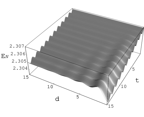
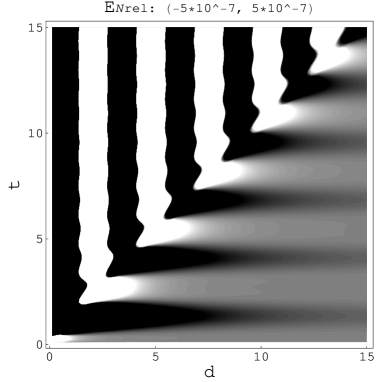
Figure 1: The zeroth-order results, no mutual influence is included here. $\gamma=10^{-5}$, $\Omega=2.3$, $\Lambda_{0}=\Lambda_{1}=20$, and $(\alpha,\beta)=(1.1,4.5)$. The two plots on the left are for the zeroth-order $E_{\cal N}^{(0)}$ which is seen to decrease and disentangle in time. (The behavior of $\Sigma^{(0)}$ is similar to $-E_{\cal N}^{(0)}$ but the amplitude of oscillation in time is smaller.) The two plots on the right are for the relative values of $E_{\cal N}^{(0)}$ at spatial separation $d$ to the value at infinite spatial separation, as given in $(\ref{ENrel})$. In the upper-right plot, the brighter color corresponds to the higher value of $E_{{\cal N}{\rm rel}}$.

Neglecting the mutual influences, the v-part of the zeroth-order cross correlators read

$$\left<\right.Q_{A}(t),Q_{B}(t)\left.\right>_{\rm v}^{(0)} = {\hbar\over\pi\Omega^{2}d}{\rm Re}{i\over\Omega+i\gamma}\left\{\left[\Omega+e^{-2\gamma t}\left(\Omega+2\gamma e^{i\Omega t}\sin\Omega t\right)\right]{\cal S}_{d}\right.-$$ (23)

$$\left.e^{-\gamma t}\left[\left(\Omega\cos\Omega t+\gamma\sin\Omega t\right)\left({\cal S}_{d-t}+{\cal S}_{d+t}\right)+(\Omega+i\gamma)\sin\Omega t\left({\cal C}_{d-t}-{\cal C}_{d+t}\right)\right]\right\},$$

$$\left<\right.P_{A}(t),P_{B}(t)\left.\right>_{\rm v}^{(0)} = {\hbar\over\pi\Omega^{2}d}{\rm Re}\,\,i(\Omega+i\gamma)\left\{\left[\Omega+e^{-2\gamma t}\left(\Omega-2\gamma e^{i\Omega t}\sin\Omega t\right)\right]{\cal S}_{d}\right.-$$ (24)

$$\left.e^{-\gamma t}\left[\left(\Omega\cos\Omega t-\gamma\sin\Omega t\right)\left({\cal S}_{d-t}+{\cal S}_{d+t}\right)+(\Omega-i\gamma)\sin\Omega t\left({\cal C}_{d-t}-{\cal C}_{d+t}\right)\right]\right\},$$

$$\left<\right.P_{A}(t),Q_{B}(t)\left.\right>_{\rm v}^{(0)} = \left<\right.Q_{A}(t),P_{B}(t)\left.\right>_{\rm v}^{(0)}$$ (25)

$$= {\hbar\gamma\over\pi\Omega^{2}d}e^{-\gamma t}\sin\Omega t\,\,{\rm Re}\,\,\left\{-2e^{(-\gamma+i\Omega)t}{\cal S}_{d}+{\cal S}_{d-t}+{\cal S}_{d+t}+i\left({\cal C}_{d-t}-{\cal C}_{d+t}\right)\right\},$$

where

$${\cal S}_{x} \equiv {1\over 2}({\rm Ci}[(\Omega+i\gamma)x]+{\rm Ci}[-(\Omega+i\gamma)x])\sin[(\Omega+i\gamma)x]-{\rm Si}[(\Omega+i\gamma)x]\cos[(\Omega+i\gamma)x],$$ (26)

$${\cal C}_{x} \equiv {1\over 2}({\rm Ci}[(\Omega+i\gamma)x]+{\rm Ci}[-(\Omega+i\gamma)x])\cos[(\Omega+i\gamma)x]+{\rm Si}[(\Omega+i\gamma)x]\sin[(\Omega+i\gamma)x],$$ (27)

with sine-integral Si$(x)={\rm si}(x)+\pi/2$ and cosine-integral Ci$(x)$ Arfken . The a-part of the zeroth-order correlators as well as the two-point functions (for a single inertial detector), $\left<\right.Q_{j}^{2}\left.\right>_{\rm v}^{(0)}$, $\left<\right.Q_{j},P_{j}\left.\right>_{\rm v}^{(0)}$, and $\left<\right.P_{j}^{2}\left.\right>_{\rm v}^{(0)}$ are all independent of the spatial separation $d$ [for explicit expressions see Eq. (25) in Ref. LCH08 and Appendix A in Ref. LH2006 ]. So the $d$ dependence of the zeroth-order degrees of entanglement $E_{\cal N}^{(0)}$ and $\Sigma^{(0)}$ are all coming from $(\ref{QLQRv0})$-$(\ref{PLQRv0})$, which are due to the phase difference of vacuum fluctuations that the detectors experience locally.

Note that when

$$d\to d_{\min}\equiv{1\over\Omega}e^{1-\gamma_{e}-\Lambda_{1}},$$ (28)

where $\gamma_{e}$ is the Euler constant and $\Lambda_{1}\equiv-\ln\Omega\Delta t-\gamma_{e}$ corresponds to the time-resolution $\Delta t$ of our detector theory LH2006 , one has $\left<\right.{\cal R}_{A}(t),{\cal R}_{B}(t)\left.\right>_{\rm v}^{(0)}\to\left<\right.{\cal R}_{A}(t)^{2}\left.\right>_{\rm v}^{(0)}=\left<\right.{\cal R}_{B}(t)^{2}\left.\right>_{\rm v}^{(0)}$, ${\cal R}=P,Q$. That is, the two detectors should be seen as located at the same spatial point when $d\approx d_{\min}$ in our model, which is actually a coarse-grained effective theory. Let us call $d_{min}$ the “merge distance.”

V.1 Early-time entanglement dynamics inside the light cone ($d<t$)

In the weak-coupling limit ($\gamma\Lambda_{1}\ll\Omega$), when the separation $d$ is not too small, the effect from the mutual influences comes weakly and slowly, so the zeroth-order correlators dominate the early-time behavior of the detectors. The asymptotic expansions of sine-integral and cosine-integral functions read Arfken

$${\rm Ci}[(\Omega+i\gamma)x] \approx {i\pi\over 2}\left({x\over|x|}-1\right)+{\sin(\Omega+i\gamma)x\over(\Omega+i\gamma)x},$$ (29)

$${\rm Si}[(\Omega+i\gamma)x] \approx {\pi\over 2}{x\over|x|}-{\cos(\Omega+i\gamma)x\over(\Omega+i\gamma)x},$$ (30)

for $\Omega,\gamma>0$, and $|(\Omega+i\gamma)x|\gg 1$. So in the weak-coupling limit, from $t-d=0$ up to $t-d\sim O(1/\gamma)$, one has

$$\left<\right.Q_{A}(t),Q_{B}(t)\left.\right>_{\rm v}^{(0)}\approx\theta(t-d){\sin\Omega d\over\Omega d}{\hbar\over 2\Omega}e^{-\gamma d}\left[1-e^{-2\gamma(t-d)}\right],$$ (31)

$\left<\right.P_{A}(t),P_{B}(t)\left.\right>_{\rm v}^{(0)}\approx\Omega^{2}\left<\right.Q_{A}(t),Q_{B}(t)\left.\right>_{\rm v}^{(0)}$ and $\left<\right.P_{A}(t),Q_{B}(t)\left.\right>_{\rm v}^{(0)},\left<\right.Q_{A}(t),P_{B}(t)\left.\right>_{\rm v}^{(0)}\sim O(\gamma/\Omega)$. The $\theta(t-d)$ implies the onset of a clear interference pattern ($\sim\sin\Omega d/\Omega d$) inside the light cone, as shown in Fig. 1. This is mainly due to the sign flipping of the sine-integral function ${\rm Si}_{d-t}$ in $(\ref{QLQRv0})$-$(\ref{PLQRv0})$ around $d=t$ when $d-t$ changes sign. The $\theta(t-d)$ acts like that each detector starts to “know” the existence of the other detector when they enter the light cone of each other, though the mutual influences are not considered here. In the next subsection we will see that there exists some interference pattern of $O(\gamma)$ in $\Sigma$ even for $d>t$, where no classical signal can reach one detector from the other.

V.2 Outside the light cone ($d>t$)

Before the first mutual influences from one detector reaches the other, the zeroth-order results are exact. From $(\ref{Cixgg1})$ and $(\ref{Sixgg1})$, when $d>t$ and $|\Omega+i\gamma|(d-t)\gg 1$, one has

$$\left<\right.Q_{A}(t),Q_{B}(t)\left.\right>_{\rm v}^{(0)} \approx {2\gamma\over\pi\Omega_{r}^{4}d^{2}}\left[1+e^{-2\gamma t}\left(\cos\Omega t+{\gamma\over\Omega}\sin\Omega t\right)^{2}-{2d^{2}e^{-\gamma t}\over d^{2}-t^{2}}\left(\cos\Omega t+{\gamma\over\Omega}\sin\Omega t\right)\right],$$ (32)

$$\left<\right.P_{A}(t),P_{B}(t)\left.\right>_{\rm v}^{(0)} \approx {2\gamma\over\pi d^{2}}e^{-2\gamma t}{\sin^{2}\Omega t\over\Omega^{2}},$$ (33)

$$\left<\right.P_{A}(t),Q_{B}(t)\left.\right>_{\rm v}^{(0)} = \left<\right.Q_{A}(t),P_{B}(t)\left.\right>_{\rm v}^{(0)}\approx{2\gamma e^{-\gamma t}\over\pi\Omega_{r}^{2}d^{2}}{\sin\Omega t\over\Omega}\left[-e^{-\gamma t}\left(\cos\Omega t+{\gamma\over\Omega}\sin\Omega t\right)+{d^{2}\over d^{2}-t^{2}}\right],$$ (34)

which makes the values of $E_{\cal N}$ and $\Sigma$ depend on $d$ and $t$; that is, the dependence of the degree of entanglement on the spatial separation $d$ between the two detectors varies in time $t$, even before they have causal contact with each other.

In the weak-coupling limit, with the initial state $(\ref{initGauss})$ and $\Omega\gg\gamma\Lambda_{j}>\gamma$, $j=0,1$, one has

$$E_{{\cal N}rel} \equiv -\log_{2}2c_{-}(t,d)-\left[-\log_{2}2c_{-}(t,\infty)\right]$$ (35)

$$\approx {\gamma\hbar\over\pi\ln 2}{{\cal X}\over|{\cal X}|}\sum_{n=0}^{2}{a^{\gamma}_{n}\over b_{\gamma}}\cos n\Omega t+O(\gamma^{2}\Lambda_{0},\gamma^{2}\Lambda_{1})$$

when $d>t$ and $|\Omega+i\gamma|(d-t)\gg 1$, where

$$a_{0}^{\gamma} = d^{-2}\left\{\hbar^{2}\beta^{2}+\alpha^{2}\left(-\alpha^{2}\beta^{2}\Omega^{2}+\beta^{4}+4\beta^{2}\hbar\Omega-\hbar^{2}\Omega^{2}\right)+|{\cal X}|(\alpha^{2}\Omega^{2}-\beta^{2})+\right.$$ (36)

$$\,\,\,\,\,\,\,\left.2\beta^{2}e^{-2\gamma t}\left[\hbar^{2}+\alpha^{2}(\beta^{2}-2\hbar\Omega)-|{\cal X}|\right]\right\}e^{-2\gamma t},$$

$$a_{1}^{\gamma} = -4(d^{2}-t^{2})^{-1}\beta^{2}\left\{2\alpha^{2}\hbar\Omega+\left[\hbar^{2}+\alpha^{2}(\beta^{2}-2\hbar\Omega)-|{\cal X}|\right]e^{-2\gamma t}\right\}e^{-\gamma t},$$ (37)

$$a_{2}^{\gamma} = d^{-2}\left\{4\hbar\Omega\alpha^{2}\beta^{2}+\left[\beta^{2}\hbar^{2}+\alpha^{2}\left(\alpha^{2}\beta^{2}\Omega^{2}+\beta^{4}-4\beta^{2}\hbar\Omega+\hbar^{2}\Omega^{2}\right)-|{\cal X}|(\alpha^{2}\Omega^{2}+\beta^{2})\right]e^{-2\gamma t}\right\},$$ (38)

$$b_{\gamma} = \Omega^{3}\left\{2\hbar^{2}\Omega\alpha^{2}\beta^{2}+\hbar\left[\alpha^{2}(\alpha^{2}\beta^{2}\Omega^{2}+\beta^{4}-4\beta^{2}\hbar\Omega)+(\alpha^{2}\Omega^{2}+\beta^{2})(\hbar^{2}-|{\cal X}|)\right]e^{-2\gamma t}\right.$$ (39)

$$\,\,\,\,\,\,\,\left.+(\hbar-\alpha^{2}\Omega)(\hbar\Omega-\beta^{2})(\alpha^{2}\beta^{2}+\hbar^{2}-|{\cal X}|)e^{-4\gamma t}\right\},$$

with ${\cal X}\equiv\hbar^{2}-\alpha^{2}\beta^{2}$. So for ${\cal X}\not=0$ the relative degree of entanglement at separation $d$ to those for the detectors at the same moment but separated at infinite distance oscillates in frequency $\Omega$ and/or $2\Omega$, depending on the values of $a_{n}^{\gamma}$. This explains the $(\cos\Omega t)/(d^{2}-t^{2})$ pattern outside the light cone in the upper-right plot of Fig. 1 and the small oscillations before $t\approx 7.5$ in the lower-right plot of the same figure, where $(\alpha,\beta)=(1.1,4.5)$ so $(a_{0}^{\gamma},a_{1}^{\gamma},a_{2}^{\gamma})/b^{\gamma}\approx(1.94/d^{2},-2.89/(d^{2}-t^{2}),0.95/d^{2})$ at early times. Another example is, when $(\alpha,\beta)=(1.5,0.2)$, one has $(a_{0}^{\gamma},a_{1}^{\gamma},a_{2}^{\gamma})/b^{\gamma}\approx(-4.68/d^{2},-0.06/(d^{2}-t^{2}),4.74/d^{2})$ at early times, so the $d^{-2}\cos 2\Omega t$ pattern dominates at large $d$ in the bottom-right plot of Fig. 7. For these cases, the larger the separation, the weaker the entanglement (in terms of the logarithmic negativity) at some moments, but the stronger the entanglement at other moments.

The sudden switching on of interaction at $t=0$ in our model will create additional oscillation patterns outside the light cone. However, as shown in $(\ref{ENrel})$, those oscillations are suppressed in the weak-coupling limit by $O(\gamma\Lambda_{0})$ of the above results. Here $\Lambda_{0}\equiv-\ln\Omega\Delta t_{0}-\gamma_{e}$ with $\Delta t_{0}$ corresponds to the time scale of switching on the coupling between the detectors and the quantum field (see Sec.IIIB in Ref.LH2006 for details).

When $\beta^{2}=\hbar^{2}/\alpha^{2}$ or ${\cal X}=0$, the detectors are initially separable and

$$\Sigma \approx {\hbar^{2}\over 16\alpha^{4}\pi^{2}\Omega^{4}}\left\{\pi\Omega(\hbar-\alpha^{2}\Omega)^{2}e^{-2\gamma t}(1-e^{-2\gamma t})+\right.$$ (40)

$$\left.2\gamma\Lambda_{1}\left[2\hbar\alpha^{2}\Omega(1-e^{-2\gamma t})+h^{2}e^{-2\gamma t}(1-\cos 2\Omega t)+\alpha^{4}\Omega^{2}e^{-2\gamma t}(1+\cos 2\Omega t)\right]\right\}^{2}+O(\gamma^{2}),$$

outside the light cone, which is always positive so the detectors are always separable. When we increase the coupling strength $\gamma$, we find that the values of $\Sigma$ are pushed further away from those negative values of entangled states. In Appendix B we also see that quantum entanglement is only created deep in the light cone. Therefore in our model we see no evidence of entanglement generation outside the light cone.

For $|{\cal X}|\not=0$ but sufficiently small, the detectors are initially entangled, but after a very short-time scale $O(e^{-\gamma_{e}-(\Lambda_{0}/2)})$ the value of $\Sigma$ jumps to $(\hbar^{2}\gamma\Lambda_{1}\alpha/\beta\pi)^{2}-(\hbar{\cal X}/4\alpha\beta)^{2}$, which could be positive so that the detectors become separable. In these cases quantum entanglement could revive later as $\Sigma$ is oscillating with an amplitude proportional to $\gamma\Lambda_{1}$, while these revivals of entanglement do not last more than a few periods of the intrinsic oscillation in the detectors.

V.3 Breakdown of the zeroth-order results

At late times $t\gg\gamma^{-1}$, all $\left<\right...\left.\right>_{\rm a}$ vanish, so $\left<\right...\left.\right>_{\rm v}$ dominate and the nonvanishing two-point correlation functions read

$$\left<\right.Q_{A},Q_{B}\left.\right>^{(0)}|_{t\gg\gamma^{-1}} \approx {\hbar\over\pi\Omega d}{\rm Re}{i{\cal S}_{d}\over\Omega+i\gamma},$$ (41)

$$\left<\right.P_{A},P_{B}\left.\right>^{(0)}|_{t\gg\gamma^{-1}} \approx {\hbar\over\pi\Omega d}{\rm Re}(i\Omega-\gamma){\cal S}_{d},$$ (42)

$$\left<\right.Q_{A}^{2}\left.\right>^{(0)}|_{t\gg\gamma^{-1}}=\left<\right.Q_{B}^{2}\left.\right>^{(0)}|_{t\gg\gamma^{-1}} \approx {i\hbar\over 2\pi\Omega}\ln{\gamma-i\Omega\over\gamma+i\Omega},$$ (43)

$$\left<\right.P_{A}^{2}\left.\right>^{(0)}|_{t\gg\gamma^{-1}}=\left<\right.P_{B}^{2}\left.\right>^{(0)}|_{t\gg\gamma^{-1}} \approx {\hbar\over\pi}\left\{{i\over 2\Omega}(\Omega^{2}-\gamma^{2})\ln{\gamma-i\Omega\over\gamma+i\Omega}+\gamma\left[2\Lambda_{1}-\ln\left(1+{\gamma^{2}\over\Omega^{2}}\right)\right]\right\},$$ (44)

from $(\ref{QLQRv0})$-$(\ref{PLQRv0})$ and from Ref. LH2006 .

When $d\to\infty$, the cross correlators vanish and the uncertainty relation reads

$$\Upsilon^{(0)}|_{t\gg\gamma^{-1}}\equiv\det\left[{\bf V}^{(0)}|_{t\gg\gamma^{-1}}+{i\over 2}\hbar{\bf M}\right]\approx\left(\left<\right.Q_{A}^{2}\left.\right>^{(0)}\left<\right.P_{A}^{2}\left.\right>^{(0)}|_{t\gg\gamma^{-1}}-{\hbar^{2}\over 4}\right)^{2}\geq 0,$$ (45)

for sufficiently large $\Lambda_{1}$ LH2006 , so the uncertainty relation holds perfectly. However, observing that $\left|{\cal S}_{d}\right|\approx\pi e^{-\gamma d}$ for $d$ large enough but still finite, the late-time $\Upsilon^{(0)}$ can reach the lowest values:

$$\left(\left<\right.Q_{A}^{2}(t)\left.\right>^{(0)}\left<\right.P_{A}^{2}(t)\left.\right>^{(0)}|_{t\gg\gamma^{-1}}-{\hbar^{2}\over 4}\right)^{2}+{\hbar^{4}e^{-4\gamma d}\over 16\Omega_{r}^{4}d^{4}}-$$

$${\hbar^{2}e^{-2\gamma d}\over 4d^{2}}\left[{\hbar^{2}\over 2\Omega_{r}^{2}}+\left(\left<\right.Q_{A}^{2}(t)\left.\right>^{(0)}|_{t\gg\gamma^{-1}}\right)^{2}+\Omega_{r}^{-4}\left(\left<\right.P_{A}^{2}(t)\left.\right>^{(0)}|_{t\gg\gamma^{-1}}\right)^{2}\right].$$ (46)

This zeroth-order result suggests that the uncertainty relation can fail if $d$ is not large enough to make the value of the second line of $(\ref{minU})$ overwhelmed by the first line [see Fig. 2]. When this happens the zeroth-order results break down. Therefore to describe the long-time entanglement dynamics at short distances $d$ the higher-order corrections from the mutual influences must be included for consistency.

When $\gamma\ll\gamma\Lambda_{1}\ll\Omega$, one has a simple estimate that the late-time $\Upsilon^{(0)}$ becomes negative if $d$ is smaller than about $d_{0}\approx\pi/2\Lambda_{1}\gamma$, which is much greater than $d_{ins}$ found in Sec.IV.

Figure 2: The oscillating curve represents the value of $\Upsilon^{(0)}$ (defined in $(\ref{0thUnc})$) as a function of $d$. The bottom curve represents its lower bound (Eq.$(\ref{minU})$). It becomes negative when $d<616$, which signifies the violation of uncertainty relation. To rectify this, one needs to add on the mutual influences, as shown in Fig. 3. Here $\gamma=10^{-4}$, $\Omega=2.3$, $\Lambda_{0}=\Lambda_{1}=25$.

VI Entanglement at late times

Since all $q_{i}^{(j)}$ vanish at late times in the stable regime (see Appendix A), the late-time correlators consist of $q_{j}^{(\pm)}$ only, for example,

$$\left<\right.Q_{B}^{2}\left.\right>|_{t\to\infty}=\int{\hbar d^{3}k\over(2\pi)^{3}2\omega}q_{B}^{(+)}(t,{\bf k})q_{B}^{(-)}(t,{\bf k})|_{t\to\infty},$$ (47)

where $q_{B}^{(+)}(t,{\bf k})|_{t\to\infty}$ is given by $(\ref{lateTqp})$ and $q_{B}^{(-)}(t,{\bf k})|_{t\to\infty}$ is its complex conjugate. After some algebra, we find that the value of the nonvanishing correlators at late times can be written as

$$\left<\right.Q_{A}^{2}\left.\right>|_{t\to\infty}=\left<\right.Q_{B}^{2}\left.\right>|_{t\to\infty} = 2{\rm Re}\left({\cal F}_{0+}+{\cal F}_{0-}\right),$$ (48)

$$\left<\right.Q_{A},Q_{B}\left.\right>|_{t\to\infty} = 2{\rm Re}\left({\cal F}_{0+}-{\cal F}_{0-}\right),$$ (49)

$$\left<\right.P_{A}^{2}\left.\right>|_{t\to\infty}=\left<\right.P_{B}^{2}\left.\right>|_{t\to\infty} = 2{\rm Re}\left({\cal F}_{2+}+{\cal F}_{2-}\right),$$ (50)

$$\left<\right.P_{A},P_{B}\left.\right>|_{t\to\infty} = 2{\rm Re}\left({\cal F}_{2+}-{\cal F}_{2-}\right),$$ (51)

where

$${\cal F}_{c\pm}(\gamma,\Omega,d)\equiv{\hbar i\over 4\pi}\int_{0}^{\omega_{max}}d\omega{\omega^{c}\over\omega^{2}+2i\gamma\omega-\Omega_{r}^{2}\pm{2\gamma\over d}e^{i\omega d}},$$ (52)

and $\omega_{max}$ is the high frequency (UV) cutoff corresponding to $\Lambda_{1}$.

In the stable regime one can write ${\cal F}_{c\pm}$ in a series form:

$${\cal F}_{c\pm}(\gamma,\Omega,d) = {\hbar i\over 4\pi}\int_{0}^{\omega_{max}}d\omega{\omega^{c}\over\omega^{2}+2i\gamma\omega-\Omega^{2}-\gamma^{2}}\sum_{n=0}^{\infty}\left[{\mp{2\gamma\over d}e^{i\omega d}\over\omega^{2}+2i\gamma\omega-\Omega^{2}-\gamma^{2}}\right]^{n}$$ (53)

$$= {\hbar i\over 4\pi}\int_{0}^{\omega_{max}}d\omega\sum_{n=0}^{\infty}{1\over n!}\left[\mp{\gamma\over\Omega d}e^{i\omega d}\partial_{\Omega}\right]^{n}{\omega^{c}\over\omega^{2}+2i\gamma\omega-\Omega^{2}-\gamma^{2}},$$

so we have

$${\cal F}_{0\pm}(\gamma,\Omega,d) = {\hbar\over 4\pi}\left\{{i\over 2\Omega}\ln{\gamma-i\Omega\over\gamma+i\Omega}+\sum_{n=1}^{\infty}{1\over n!}\left[\mp{\gamma\over\Omega d}\partial_{\Omega}\right]^{n}{\rm Re}\,{i\over\Omega}e^{(\gamma+i\Omega)nd}\Gamma[0,(\gamma+i\Omega)nd]\right\},$$ (54)

$${\cal F}_{2\pm}(\gamma,\Omega,d) = {\hbar\over 4\pi}\left\{{i\over 2\Omega}\left(\Omega^{2}-\gamma^{2}\right)\ln{\gamma-i\Omega\over\gamma+i\Omega}+\gamma\left[2\Lambda_{1}-\ln\left(1+{\gamma^{2}\over\Omega^{2}}\right)\right]+\right.$$ (55)

$$\left.\sum_{n=1}^{\infty}{1\over n!}\left[\mp{\gamma\over\Omega d}\partial_{\Omega}\right]^{n}{\rm Re}{i\over\Omega}e^{(\gamma+i\Omega)nd}(\gamma+i\Omega)^{2}\Gamma[0,(\gamma+i\Omega)nd]\right\},$$

for large frequency cutoff $\omega_{max}$, or the corresponding $\Lambda_{1}$.

Substituting the late-time correlators $(\ref{LTQ2})$-$(\ref{LTPx})$ into the covariance matrix ${\bf V}$, we get

$$\Sigma|_{t\to\infty} = \left(16{\rm Re}{\cal F}_{0+}{\rm Re}{\cal F}_{2-}-{\hbar^{2}\over 4}\right)\left(16{\rm Re}{\cal F}_{0-}{\rm Re}{\cal F}_{2+}-{\hbar^{2}\over 4}\right),$$ (56)

$$\Upsilon|_{t\to\infty} = \left(16{\rm Re}{\cal F}_{0+}{\rm Re}{\cal F}_{2+}-{\hbar^{2}\over 4}\right)\left(16{\rm Re}{\cal F}_{0-}{\rm Re}{\cal F}_{2-}-{\hbar^{2}\over 4}\right).$$ (57)

Numerically we found that $16{\rm Re}{\cal F}_{0+}{\rm Re}{\cal F}_{2-}-(\hbar^{2}/4)$ and $\Upsilon|_{t\to\infty}$ are positive definite in the cases considered in this paper. We then identify the late-time symplectic spectrum $(c_{+},c_{-})|_{t\to\infty}=(4\sqrt{{\rm Re}{\cal F}_{0+}{\rm Re}{\cal F}_{2-}},4\sqrt{{\rm Re}{\cal F}_{0-}{\rm Re}{\cal F}_{2+}})$. So if $16{\rm Re}{\cal F}_{0+}{\rm Re}{\cal F}_{2-}-(\hbar^{2}/4)$ is negative, then $\Sigma<0$, $E_{\cal N}>0$, and the detectors are entangled.

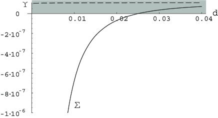
Figure 3: Plots for $\Sigma$ (solid curve) and $\Upsilon$ (dashed curve) at late times as a function of $d$, with parameters the same as those in Fig. 2. Two detectors are separable when $\Sigma\geq 0$ (shaded zone). One can see that $\Sigma$ becomes negative when $d<0.025$. With the mutual influences included, the uncertainty relation [see Eq.$(\ref{Uncert})$ and below] now holds for all $d$.

In the weak-coupling limit, keeping the correlators to $O(\gamma/d)$, we have

$$16{\rm Re}{\cal F}_{0+}{\rm Re}{\cal F}_{2-}-{\hbar^{2}\over 4} \approx {\hbar^{2}\gamma\Lambda_{1}\over\pi\Omega}-{\hbar^{2}\over\Omega^{3}}{\rm Re}\left\{\left[{i\gamma\Omega\over\pi d}+{2\gamma^{2}\Lambda_{1}\over\pi^{2}d}(i+\Omega d)\right]e^{i\Omega d}\Gamma[0,i\Omega d]\right\},$$ (58)

which is positive as $d\to\infty$, but negative when $d\to 0_{+}$. So $(\ref{soldent})$ must cross zero at a finite “entanglement distance” $d_{ent}>0$, where $\Sigma=0$. For $d<d_{ent}$, the detectors will have residual entanglement, while for $d>d_{ent}$, the detectors are separable at late times.

For small $\gamma$, $d_{ent}$ is almost independent of $\gamma$. We find that when $\gamma\Lambda_{1}\ll\Omega$ and $\Lambda_{1}\gg 1$,

$$d_{ent}\approx{\pi/2\Omega\over\Lambda_{1}-\ln{\pi\over 2\Lambda_{1}}}.$$ (59)

will be a good estimate if $d_{ent}\ll 1$. Here $d_{ent}$ is still much larger than the “merge distance” $d_{min}$ in $(\ref{dmin})$. For example, as shown in Fig. 3, when $\gamma=0.0001$, $\Omega=2.3$, $\Lambda_{1}=25$, one has $d_{ent}\approx 0.025$, which is quite a bit greater than the “radius of instability” $2\gamma/\Omega_{r}^{2}\approx 3.8\times 10^{-5}$, and much greater than the merge distance $d_{min}\approx 9\times 10^{-12}$.

A corollary follows. If the initial state of the two detectors with $d<d_{ent}$ is separable, then the residual entanglement implies that there is an entanglement creation during the evolution. In contrast, if the initial state of the two detectors with $d>d_{ent}$ is entangled, then the late-time separability implies that they disentangled in a finite time. Examples will be given in the next section.

Note that the ill behavior of $\Upsilon^{(0)}$ has been cured by mutual influences. The uncertainty function $(\ref{lateUnc})$ is positive for all $d$ at late times.

Note also that, while the corrections from the mutual influences to $\left<\right.Q_{A}^{2}\left.\right>|_{t\to\infty}$ and $\left<\right.P_{A}^{2}\left.\right>|_{t\to\infty}$ are $O(\gamma/d)$, the mutual influences have been included in the leading order approximation for the cross correlators. Indeed, in $(\ref{Fseries})$, even as low as $n=1$, we have had

$$\left<\right.Q_{A},Q_{B}\left.\right>|_{t\to\infty} \approx \left<\right.Q_{A},Q_{B}\left.\right>^{(0)}|_{t\to\infty}-{2\hbar\gamma\over\pi}{4\gamma\over d}\int_{0}^{\infty}d\omega{\omega\left[(\Omega^{2}_{r}-\omega^{2})\cos\omega d-2\gamma\omega\sin\omega d\right]\over\left[(\omega^{2}-\Omega^{2}_{r})^{2}+4\gamma^{2}\omega^{2}\right]^{2}}.$$ (60)

However, this is slightly different from the approximation with the first-order mutual influences included. Writing the $n=0$ and $n=1$ terms in Eq. $(\ref{qjp})$ as

$$q_{j}^{(+)}\approx q_{j,n=0}^{(+)}+q_{j,n=1}^{(+)},$$ (61)

then the approximated cross correlator with the first-order mutual influences included is the $\omega$ integration of Re $[(q_{A,n=0}^{(+)}+q_{A,n=1}^{(+)})(q_{B,n=0}^{(+)}+q_{B,n=1}^{(+)})]$, but in $(\ref{1stgamma})$ only Re $[q_{A,n=0}^{(+)}q_{B,n=0}^{(+)}+q_{A,n=0}^{(+)}q_{B,n=1}^{(+)}+q_{A,n=1}^{(+)}q_{B,n=0}^{(+)}]$ contribute, though there are $O(\gamma^{0})$ terms in $q_{A,n=1}^{(+)}q_{B,n=1}^{(+)}$. The latter is small for $\Omega d\gg 1$, and will be canceled by the mutual influences of higher-orders.

VII Entanglement dynamics in weak-coupling limit

VII.1 Disentanglement at very large distance

Suppose the two detectors are separated far enough $(d\gg\Omega)$ so that the cross correlations and the mutual influences can be safely ignored. Then in the weak-coupling limit ($\Omega\gg\gamma\Lambda_{1}$) the zeroth-order results for the v-part of the self correlators dominate, so that LCH08

$$\left<\right.Q_{A}^{2}\left.\right>_{\rm v}=\left<\right.Q_{B}^{2}\left.\right>_{\rm v} \approx {\hbar\over 2\Omega}\left(1-e^{-2\gamma t}\right),$$ (62)

$$\left<\right.P_{A}^{2}\left.\right>_{\rm v}=\left<\right.P_{B}^{2}\left.\right>_{\rm v} \approx {\hbar\over 2}\Omega\left(1-e^{-2\gamma t}\right)+{2\over\pi}\hbar\gamma\Lambda_{1},$$ (63)

and $\left<\right.Q_{A},P_{A}\left.\right>_{\rm v}=\left<\right.Q_{B},P_{B}\left.\right>_{\rm v}\sim O(\gamma)$, while the v-part of the cross correlators are vanishingly small. This is exactly the case we have considered in Sec. IV A 2 of Ref. LCH08 , where we found

$$\Sigma\approx{\hbar^{2}e^{-4\gamma t}\over 16\alpha^{2}\beta^{2}\Omega^{2}}\left[Z_{8}\left(e^{-4\gamma t}-2e^{-2\gamma t}\right)+Z_{4}\right]+{\hbar^{3}\gamma\Lambda_{1}\over 4\pi\alpha^{2}\beta^{2}\Omega^{2}}Z_{2}e^{-2\gamma t}+{\hbar^{4}\over\pi^{2}\Omega^{2}}\gamma^{2}\Lambda_{1}^{2},$$ (64)

with $Z_{8}\geq 0$, $Z_{8}-Z_{4}\geq 0$ and $Z_{2}\geq 0$ [$Z_{8}$, $Z_{4}$ and $Z_{2}$ are parameters depending on $\alpha$ and $\beta$, defined in Eqs.$(37)$, $(38)$ and $(41)$ of Ref. LCH08 , respectively.] Accordingly the detectors always disentangle in a finite time. There are two kinds of behaviors that $\Sigma$ could have. For $Z_{4}>0$, the disentanglement time is a function of $Z_{4}$, $Z_{8}$ and $\gamma$,

$$t^{(0)}_{dE>}\approx-{1\over 2\gamma}\ln\left(1-\sqrt{1-{Z_{4}\over Z_{8}}}\right),$$ (65)

while for $Z_{4}<0$, the disentanglement time is much longer,

$$t^{(0)}_{dE<}\approx{1\over 2\gamma}\ln{|Z_{4}|\pi/(2\hbar\gamma\Lambda_{1})\over Z_{2}+\sqrt{Z_{2}^{2}-4\alpha^{2}\beta^{2}Z_{4}}},$$ (66)

and depends on $\Lambda_{1}$.

VII.2 Disentanglement at large distance

When $d$ is large (so $1/\Omega d$ is small) but not too large to make all the mutual influences negligible, while the zeroth-order results for the v-part of the self-correlators $(\ref{Q2weak0})$ and $(\ref{P2weak0})$ are still good, the first-order correction [$n=1$ terms in (14)] to the cross correlators $\left<\right.Q_{A},Q_{B}\left.\right>$ can be of the same order of $\left<\right.Q_{A},Q_{B}\left.\right>^{(0)}$ (a similar observation on the late-time correlators has been mentioned in the end of Sec. VI). Including the first-order correction, for $d>O(1/\sqrt{\gamma\Omega})$, we have a simple expression,

$$\left<\right.Q_{A},Q_{B}\left.\right>_{\rm v} = \left<\right.Q_{A},Q_{B}\left.\right>^{(0)}_{\rm v}+\theta(t-d){\hbar\over 2\Omega}{\sin\Omega d\over\Omega d}e^{-\gamma d}\left[-1+e^{-2\gamma(t-d)}\left(1+2(t-d)\gamma\right)+O(\gamma/\Omega)\right]$$ (67)

$$\approx \theta(t-d){\hbar\over\Omega}{\sin\Omega d\over\Omega d}e^{-\gamma d}\gamma(t-d)e^{-2\gamma(t-d)},$$

and $\left<\right.P_{A},P_{B}\left.\right>_{\rm v}\approx\Omega^{2}\left<\right.Q_{A},Q_{B}\left.\right>_{\rm v}$ with other two-point functions $\left<\right...\left.\right>_{\rm v}$ being $O(\gamma)$ for all $t$. Here $\left<\right.Q_{A},Q_{B}\left.\right>^{(0)}_{\rm v}$ in the weak-coupling limit has been shown in $(\ref{QLQRv0wcl})$. The above approximation is good over the time interval from $t=0$ up to $e^{-2\gamma(t-d)}>O(\gamma/\Omega)$, namely, before $t-d\sim O(-\gamma^{-1}\ln(\gamma/\Omega))$.

Still, in this first-order approximation, $\left<\right.Q_{A},Q_{B}\left.\right>_{\rm v}$ and $\left<\right.P_{A},P_{B}\left.\right>_{\rm v}$ are the only correlators depending on the separation $d$. Inserting those approximated expressions for the correlators into the definition of $\Sigma$ or $E_{\cal N}$, we find that the interference pattern in $d$ for the relative values of $\Sigma$ or $E_{\cal N}$ at early times (Fig. 1) can last through the disentanglement process to make the disentanglement time $t_{dE}$ longer or shorter than those at $d\to\infty$, though the contrast decays noticeably compared with those at early times. Two examples are shown in Fig. 4. For $Z_{4}>0$, the disentanglement time is about

$$t_{dE>}\approx t^{(0)}_{dE>}-{Z_{6}\left(t^{(0)}_{dE>}-d\right)e^{\gamma d}\sin\Omega d\over Z_{8}d\left(1-e^{-2\gamma t^{(0)}_{dE>}}\right)+Z_{6}\left[1-2\gamma\left(t^{(0)}_{dE>}-d\right)\right]e^{\gamma d}\sin\Omega d},$$ (68)

where $Z_{6}\equiv(\hbar^{2}-\alpha^{2}\beta^{2})(\alpha^{2}\Omega^{2}-\beta^{2})$ [Fig. 4 (left)]. In this case the disentanglement time can be short compared to the time scale $O(n/\gamma)$, $n\in N$ when the higher-order corrections $q_{n}$ from mutual influences reach their maximum values (see Sec. III). So in the weak-coupling limit the above estimate could be good from large $d$ all the way down to $\Omega d\sim O(1)$ but still much greater than $\Omega d_{ent}$. If this is true, the difference of disentanglement times for different spatial separations can be significant at small $d$. For example, for $(\alpha,\beta)=(1.5,0.2)$ with other parameters the same as those in Fig. 4, the disentanglement time at $d\approx 4.4934/\Omega$ (where $\sin\Omega d/\Omega d$ is the global minimum) is over $1.6$ times longer than those for $d\approx 7.7253/\Omega$ (where the first peak of $\sin\Omega d/\Omega d$ is located).

For $Z_{4}<0$, the correction of $\sin\Omega d$ is below the precision of $t^{(0)}_{dE<}$ estimated in $(\ref{tdEZ4n})$. Here we just show the numerical result up to the first-order mutual influences in Fig. 4 (right), which shows that the interference pattern in $d$ is suppressed but still nonvanishing for large disentanglement times.

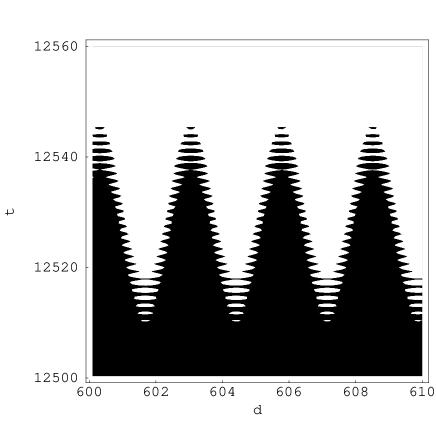
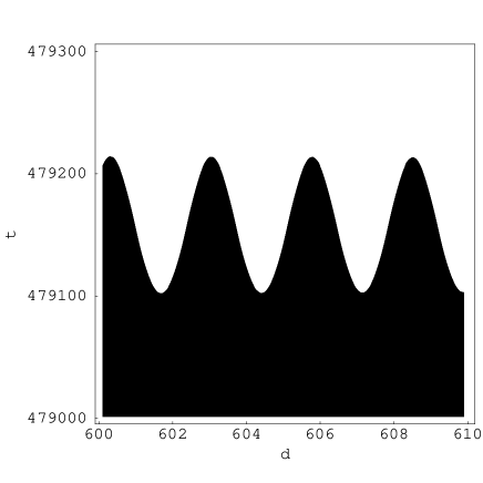
Figure 4: The plot of $\Sigma$ as a function of $d$ and $t$, up to the first-order correction. $\Sigma$ is negative in the dark region and positive in the bright region. For a fixed $d$, the disentanglement time $t_{dE}$ is at the border of the lowest dark region or the earliest time that the detectors becomes separable. The interference pattern in Fig. 1 for $\Sigma$ at early times signifies that the disentanglement time $t_{dE}$ is longer or shorter than those at $d\to\infty$ [Eqs. (65] and ($\ref{tdEZ4n})$). The gridded profile in the left plot shows that after $t_{dE}$ there could be some short-time revivals of entanglement. Here the parameters are the same as those in Fig. 1 except $(\alpha,\beta)=(1.5,0.2)$ in the left plot and $(1.1,4.5)$ in the right (cf. Fig. 3 in Ref. LCH08 ).

VII.3 Entanglement generation at very short distance

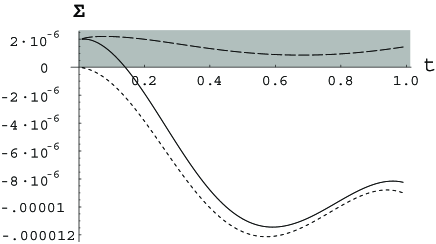
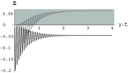
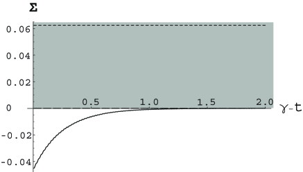
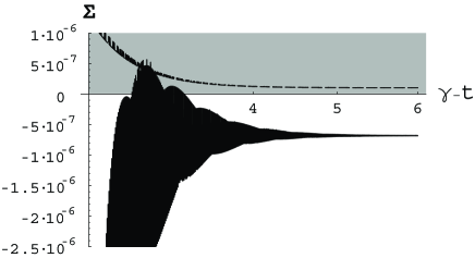
Figure 5: (Upper left) The solid curve and the long-dashed curve represent the values of $\Sigma$ and $\Upsilon$, respectively, while the dotted line is for the value of $\Sigma$ with all $\left<\right...\left.\right>_{\rm v}$ set to zero. The detectors are separable initially (the parameters here are the same as those in Figs. 2 and 3 except $d=0.01$ and $(\alpha,\beta)=(1,1)$). Quantum entanglement has been generated after $t\approx 0.15$, and $\Sigma$ oscillates in frequency $\Omega_{+}$ at early times. Around the time scale $t\sim 1/\gamma_{+}$ ($\approx 5000$ here) (upper right), $\Sigma$ has an oscillation with long period $\pi/(\Omega_{-}-\Omega_{+})$ $(\approx 361.4)$. $\Sigma$ appears to be settling down at a value (about $-0.046$ here) depending in this case only on the value $\alpha$ in the initial data. However, in a much longer time scale $t\sim 1/\gamma_{-}$ ($\approx 1.13\times 10^{8}$) (lower left), one sees that the value of $|\Sigma|$ is actually decaying exponentially to the late-time value ($\approx-6.8\times 10^{-7}$) consistent with the results in Fig. 3 with $d=0.01$ and independent of the initial data of the detectors.

When $\Omega d\sim O(\epsilon)$, $\gamma/\Omega\sim O(\epsilon^{2})$, and $\epsilon\ll 1$, one can perform a dimensional reduction on the third derivatives in $(\ref{eomsmalld})$, namely,

$$\dddot{q}_{\pm}^{(j)}\approx-{\Omega_{r}^{2}\mp{2\gamma\over d}\over 1\mp\gamma d}\dot{q}_{\pm}^{(j)},$$ (69)

to obtain, up to $O(\epsilon^{5})$,

$$\ddot{q}^{(j)}_{\pm}+2\gamma_{\pm}\dot{q}^{(j)}_{\pm}+\Omega^{2}_{\pm}\dot{q}^{(j)}_{\pm} \approx 0,$$ (70)

$$\ddot{q}^{(+)}_{\pm}+2\gamma_{\pm}\dot{q}^{(+)}_{\pm}+\Omega^{2}_{\pm}\dot{q}^{(+)}_{\pm} \approx \lambda_{\pm}\left(e^{-ik_{1}d/2}\pm e^{ik_{1}d/2}\right)e^{-i\omega t},$$ (71)

where $j=A,B$, $q_{\pm}^{(+)}\equiv q_{A}^{(+)}\pm q_{B}^{(+)}$ and

$$\gamma_{-} \equiv {\gamma d^{2}\over 6}{\left(\Omega_{r}^{2}+{2\gamma\over d}\right)\over(1+\gamma d)^{2}},$$ (72)

$$\gamma_{+} \equiv {2\gamma\over 1-\gamma d}-{\gamma d^{2}\over 6}{\left(\Omega_{r}^{2}-{2\gamma\over d}\right)\over(1-\gamma d)^{2}},$$ (73)

$$\Omega^{2}_{\pm} \equiv {\Omega_{r}^{2}\mp{2\gamma\over d}\over 1\mp\gamma d},\,\,\,\,\,\lambda_{\pm}\equiv{\lambda_{0}\over 1\mp\gamma d}.$$ (74)

Here $\gamma_{-}/\gamma_{+}$ is of $O(\epsilon^{2})$. Note that $q_{-}^{j}$ and the decay modes in $q_{-}^{(+)}$ have subradiant behavior, while $q_{+}^{j}$ and the decay modes in $q_{+}^{(+)}$ are superradiant. For small $d$, the time scale $\gamma_{-}^{-1}\gg\gamma^{-1}>\gamma_{+}^{-1}\approx 1/2\gamma$, and $\gamma_{-}^{-1}$ goes to infinity as $d\to 0$.

The solutions for $(\ref{eomqje5})$ and $(\ref{eomqpme5})$ with suitable initial conditions are

$$q_{j}^{(j)}\pm\bar{q}_{j}^{(j)} = {1\over 2}e^{-\gamma_{\pm}t}\left[s_{1}^{\pm}e^{i\Omega_{\pm}t}+s_{2}^{\pm}e^{-i\Omega_{\pm}t}\right],$$ (75)

$$q_{A}^{(+)}\pm q_{B}^{(+)} = {\lambda_{\pm}\over\Omega_{\pm}}\left(e^{-ik_{1}d/2}\pm e^{ik_{1}d/2}\right)\left[\left(M_{1}^{\pm}-M_{2}^{\pm}\right)e^{-i\omega t}+e^{-\gamma_{\pm}t}\left(M_{2}^{\pm}e^{i\Omega_{\pm}t}-M_{1}^{\pm}e^{-i\Omega_{\pm}t}\right)\right],$$ (76)

where $s_{1}^{\pm}\equiv[1-\Omega_{\pm}^{-1}(\Omega_{r}+i\gamma_{\pm})]/2$, $s_{2}^{\pm}\equiv[1+\Omega_{\pm}^{-1}(\Omega_{r}+i\gamma_{\pm})]/2$, $M_{1}^{\pm}\equiv(-\omega-i\gamma_{\pm}+\Omega_{\pm})^{-1}$, and $M_{2}^{\pm}\equiv(-\omega-i\gamma_{\pm}-\Omega_{\pm})^{-1}$. Actually these solutions are the zeroth-order results with $\gamma$ and $\Omega$ replaced by $\gamma_{\pm}$ and $\Omega_{\pm}$. So we can easily reach the simple expressions

$$\left<\right.Q_{A}^{2}\left.\right>_{\rm v} \approx {\lambda_{+}^{2}\over 16\pi\gamma_{+}}\left[\left<\right.Q_{A}^{2}\left.\right>_{\rm v}^{(0)}+\left<\right.Q_{A},Q_{B}\left.\right>_{\rm v}^{(0)}\right]_{\gamma\to\gamma_{+}}^{\Omega\to\Omega_{+}}+{\lambda_{-}^{2}\over 16\pi\gamma_{-}}\left[\left<\right.Q_{A}^{2}\left.\right>_{\rm v}^{(0)}-\left<\right.Q_{A},Q_{B}\left.\right>_{\rm v}^{(0)}\right]_{\gamma\to\gamma_{-}}^{\Omega\to\Omega_{-}},$$ (77)

$$\left<\right.Q_{A},Q_{B}\left.\right>_{\rm v} \approx {\lambda_{+}^{2}\over 16\pi\gamma_{+}}\left[\left<\right.Q_{A},Q_{B}\left.\right>_{\rm v}^{(0)}+\left<\right.Q_{A}^{2}\left.\right>_{\rm v}^{(0)}\right]_{\gamma\to\gamma_{+}}^{\Omega\to\Omega_{+}}+{\lambda_{-}^{2}\over 16\pi\gamma_{-}}\left[\left<\right.Q_{A},Q_{B}\left.\right>_{\rm v}^{(0)}-\left<\right.Q_{A}^{2}\left.\right>_{\rm v}^{(0)}\right]_{\gamma\to\gamma_{-}}^{\Omega\to\Omega_{-}},$$ (78)

and so on. Here $\left<\right...\left.\right>_{\rm v}^{(0)}$ are those expressions given in $(\ref{QLQRv0})$-$(\ref{PLQRv0})$ above and in Eqs.(A9) and (A10) of Ref.LH2006 ($\left<\right.Q_{A},P_{A}\left.\right>_{\rm v}=\partial_{t}\left<\right.Q_{A}^{2}\left.\right>_{\rm v}/2$.) The prefactors $\lambda_{\pm}^{2}/16\pi\gamma_{\pm}$ are put there because in our definitions for the zeroth-order results the overall factor $\lambda_{0}^{2}$ has been expressed in terms of $8\pi\gamma$, but now $\gamma_{\pm}\not=\lambda_{\pm}/8\pi$.

In Fig. 5 we demonstrate an example in which the two detectors are separable in the beginning but get entangled at late times. There are three stages in their history of evolution:

1. At a very early time ($t\approx 0.15$) quantum entanglement has been generated. This entanglement generation is dominated by the mutual influences sourced by the initial information in the detectors and mediated by the field. (For more early-time analysis, see Appendix B.)

2. Then around the time scale $t\sim 1/\gamma_{+}$, the contribution from vacuum fluctuations of the field ($\left<\right...\left.\right>_{\rm v}$) takes over so that $\Sigma$ becomes quasisteady and appears to settle down at a value depending on part of the initial data of the detectors. More explicitly, at this stage $q_{+}^{(\mu)}$, $\mu=A,B,+,-$ have been in their late-time values but $q_{-}^{(\mu)}$ are still about their initial values, so

$$\Sigma|_{t\sim 1/\gamma_{+}}\approx{\hbar^{4}\over 64}\left[{\sin\Omega d\over\Omega d}e^{-2\gamma d}+1-{2\over\hbar}\alpha^{2}\Omega\right]\left[{\sin\Omega d\over\Omega d}e^{-2\gamma d}+1-{2\hbar\over\alpha^{2}\Omega}+{8\Lambda_{1}\gamma\over\pi\Omega}\right]$$ (79)

in the weak-coupling and short distance approximation $\gamma\ll d\Omega^{2}\ll\Omega$. Here $\Sigma$ depends on $\alpha$ only. The parameter $\beta$ in initial state $(\ref{initGauss})$ is always associated with $q_{+}^{(j)}$ in $\left<\right...\left.\right>_{\rm a}$ so it becomes negligible at this stage [cf. Eq.(25) in LCH08 ]. Note that $\Sigma|_{t\sim 1/\gamma_{+}}$ can be positive for small $d$ only when $\alpha$ is at the neighborhood of $\sqrt{\hbar/\Omega}$.

3. The remaining initial data persist until a much longer time scale $t\sim 1/\gamma_{-}$ when $\Sigma$ approaches a value consistent with the late-time results given in Sec. VI, which are contributed purely by the vacuum fluctuations of the field and independent of any initial data in the detectors. In this example the detectors have residual entanglement, though small compared to those in stage 2.

The above behaviors in stages 2 and 3 cannot be obtained by including only the first-order correction from the mutual influences. Thus in this example we conclude that the mutual influences of the detectors at very short distance generate a transient entanglement between them in midsession, while vacuum fluctuations of the field with the mutual influences included give the residual entanglement of the detectors at late times.

For the detectors initially entangled, only the early-time behavior looks different from the above descriptions. Their entanglement dynamics are similar to the above in the second and the third stages.

VIII Discussion

VIII.1 Physics represented by length scales

The physical behavior of the system we studied may be characterized by the following length scales:

Merge distance $d_{min}$ in Eq.(28).–Two detectors separated at a distance less than $d_{min}$ would be viewed as those located at the same spatial point;

Radius of instability $d_{ins}$ in Eq.(22).–For any two detectors at a distance less than $d_{ins}$, their mode functions will grow exponentially in time so the quantum fluctuations of the detector diverge at late times;

Entanglement distance $d_{ent}$ in Eq.$(\ref{dentdef})$.–Two detectors at a distance less than $d_{ent}$ will be entangled at late times, otherwise separable;

And $d_{0}$ defined in Sec. V.3.–For $d<d_{0}$ the zeroth-order results breakdown. A stable theory should have $d_{ent}$ and $d_{min}$ greater than $d_{ins}$.

VIII.2 Direct interaction and effective interaction

In a closed bipartite system a direct interaction between the two parties, no matter how weak it is, will generate entanglement at late times. However, as we showed above, an effective interaction between the two detectors mediated by quantum fields will not generate residual entanglement (though creating transient entanglement is possible) if the two detectors are separated far enough, where the strength of the effective interactions is weak but not vanishing.

VIII.3 Comparison with 2HO QBM results

When $d\to d_{min}$ with large enough $\Omega$, our model will reduce to a 2HO QBM model with real renormalized natural frequencies for the two harmonic oscillators. Paz and Roncaglia PR07 have studied the entanglement dynamics of this 2HO QBM model and found that, at zero temperature, for both oscillators with the same natural frequency, there exists residual entanglement at late times in some cases and infinite sequences of sudden death and revival in other cases. In the latter case the averaged asymptotic value of negativity is still positive and so the detectors are “entangled on average.”

While our results show that the late-time behavior of the detectors is independent of the initial state of the detectors, the asymptotic value of the negativity at late times in PR07 does depend on the initial data in the detectors (their initial squeezing factor). This is because in PR07 the two oscillators are located exactly at the same point, namely, $d=0$, so $\gamma_{-}=0$ and the initial data carried by $q_{-}^{(j)}$ persists forever. Since in our cases $d$ is not zero, the “late” time in PR07 actually corresponds to the time interval with $(1/\gamma_{+})\ll t\ll(1/\gamma_{-})$ in our cases, which is not quite late for our detectors.

VIII.4 Where is the spatial dependence of entanglement coming from?

Two factors are responsible for the spatial dependence of entanglement. The first one is the phase difference of vacuum fluctuations that the two detectors experience. This is mainly responsible for the entanglement outside the light cone in all coupling strengths and those inside the light cone with sufficiently large separation in the weak-coupling limit, such as the cases in Sec.V. The second factor is the interference of retarded mutual influences, which are generated by backreaction from the detectors to the field. It is important in the cases with small separation between the detectors, such as those in Sec.VII.3.

VIII.5 Non-Markovian behavior and strong coupling

In our prior work LH2006 and LCH08 , the non-Markovian behavior arises mainly from the vacuum fluctuations experienced by the detectors, and the essential temporal nonlocality in the autocorrelation of the field at zero temperature manifests fully in the strong-coupling regime. Nevertheless, in Sec. VII.3 one can see that, even in the weak-coupling limit, once the spatial separation is small enough and the evolution time is long enough, the mutual influences will create some non-Markovian behavior very different from those results obtained from perturbation theory with higher-order mutual influences on the mode functions neglected.

Acknowledgement S.Y.L. wishes to thank Jen-Tsung Hsiang for helpful discussions. This work is supported in part by grants from the NSF Grants No. PHY-0426696, No. PHY-0601550, No. PHY-0801368, and the Laboratory for Physical Sciences.

Appendix A Late-time analysis on mode functions

Let

$$q_{+}^{(A)}(t)=\sum_{j}c_{j}e^{iK_{j}t},$$ (80)

Equation (18) gives

$$\sum_{j}c_{j}\left[-K_{j}{}^{2}+2i\gamma K_{j}+\Omega_{r}^{2}\right]e^{iK_{j}t}={2\gamma\over d}\sum_{j^{\prime}}c_{j^{\prime}}e^{iK_{j^{\prime}}(t-d)}.$$ (81)

At late times, one is allowed to perform the Fourier transformation on both sides with $t$ integrations over $(-\infty,\infty)$ to obtain

$$-K_{j}^{2}+2i\gamma K_{j}+\Omega_{r}^{2}={2\gamma\over d}e^{-iK_{j}d}.$$ (82)

There are infinitely many solutions for $K_{j}$ in the complex $K$ plane, so one needs infinitely many initial conditions to fix the factors $c_{j}$. Our $q_{+}$ chosen as a free oscillator at the initial moment and unaffected by its own history until $t=d$ in principle can be specified by a set of $c_{j}$’s. Suppose this is true. Writing $K_{j}\equiv x_{j}+iy_{j}$, the real and imaginary parts of $(\ref{eomK})$ then read

$$(y-\gamma)^{2}-x^{2}+\Omega^{2} = {2\gamma\over d}e^{yd}\cos xd,$$ (83)

$$x(y-\gamma) = {\gamma\over d}e^{yd}\sin xd.$$ (84)

The solutions for them are shown in Fig. 6. The left-hand side of $(\ref{eomRe})$ is a saddle surface over the $xy$ space, while the right-hand side of $(\ref{eomRe})$ is exponentially growing in the $+y$ direction and oscillating in the $x$ direction. For $(\ref{eomIm})$, the situation is similar. From Fig. 6, one can see that there is no complex solution for $K$ with nonvanishing real part and negative imaginary part ($x\not=0$ and $y\leq 0$). The solutions for $K$ with its imaginary part negative must be purely imaginary. Indeed, from $(\ref{eomIm})$ and Fig. 6 (upper right), one sees that when $x\not=0$, if $y\leq 0$, then $(y-\gamma)\leq-\gamma$, but $-0.2172\gamma\lesssim\gamma e^{yd}(\sin xd)/(xd)<\gamma$, so there is no solution of $(\ref{eomIm})$ with $y\leq 0$ and $x\not=0$.

When $\Omega_{r}^{2}>2\gamma/d$, one finds that all solutions for $K$ in $(\ref{eomK})$ are located in the upper half of the complex $K$ plane, i.e., all $y_{j}>0$, which means that all modes in $(\ref{qR+FT})$ decay at late times.

When $\Omega_{r}^{2}=2\gamma/d$, there exists a solution $K=0$, with other solutions on the upper half $K$ plane. This implies that $q_{+}^{(A)}$ becomes a constant at late times.

When $\Omega_{r}^{2}<2\gamma/d$, there must exist one and only one solution for $K$ with negative $y$, which corresponds to the unstable growing mode. This is consistent with our observation in Sec.IV.

Therefore, we conclude that $q_{+}^{(A)}$ is stable and decays at late times only for $\Omega_{r}^{2}>2\gamma/d$.

As for $q_{-}^{(A)}$, from $(\ref{EOMqR-})$ it seems that $q_{-}^{(A)}$ would oscillate at late times. However, similar analysis gives the conclusion that $q_{-}^{(A)}$ decays at late times for all cases. Thus, by symmetry, all $q_{j}^{(i)}$ decay at late times in the stable regime $\Omega_{r}^{2}>2\gamma/d$.

Figure 6: (Upper left) The solutions to (82) for the complex frequency $K_{j}=x_{j}+iy_{j}$ of $q_{+}^{(A)}$ [defined in $(\ref{qR+FT})$] are located at the intersections of the dashed and solid curves, which represent the solutions to Eqs. $(\ref{eomRe})$ and $(\ref{eomIm})$, respectively. Here $\gamma=0.25$, $\Omega=0.9000202$, $d=1$. (Upper right) The same case, but here “$+$” denotes complex solutions and “$\times$” denotes purely imaginary solutions for $K$. There are two purely imaginary solutions for $K$ in this case. (Lower left) There are three purely imaginary solutions for $K$ when $\gamma=0.25$, $\Omega=0.8$, $d=1$. (Lower right) Solutions for $K$ when $\gamma=0.25$, $\Omega=0.3$, $d=1$. There is only one purely imaginary solution, which is located in the lower half of the complex $K$ plane.

Now we turn to $q^{(+)}_{A,B}$. Equation $(\ref{eomqA+2})$ implies that

$$\left(\partial_{t}^{2}+2\gamma\partial_{t}+\Omega_{r}^{2}\right)^{2}q_{B}^{(+)}(t,{\bf k}) = \left({2\gamma\over d}\right)^{2}q_{B}^{(+)}(t-2d,{\bf k})+$$ (85)

$${\lambda_{0}}e^{-i\omega t}\left[\left(-\omega^{2}-2\gamma\omega+\Omega_{r}^{2}\right)e^{ik_{1}d/2}+{2\gamma\over d}e^{i\omega d-ik_{1}d/2}\right],$$

at late times. Again, let

$$q^{(+)}_{B}(t,{\bf k})=\sum_{j}c^{j}_{\bf k}e^{iK^{j}_{\bf k}t},$$ (86)

then one has

$$\sum_{j}c^{j}_{\bf k}\left[-\left(K_{\bf k}^{j}\right)^{2}+2i\gamma K_{\bf k}^{j}+\Omega_{r}^{2}\right]^{2}e^{iK^{j}_{\bf k}t} = \sum_{j}c^{j}_{\bf k}\left({2\gamma\over d}\right)^{2}e^{iK^{j}_{\bf k}(t-2d)}+$$ (87)

$${\lambda_{0}}e^{-i\omega t}\left[\left(-\omega^{2}-2i\gamma\omega+\Omega_{r}^{2}\right)e^{ik_{1}d/2}+{2\gamma\over d}e^{i\omega d-ik_{1}d/2}\right].$$

After a Fourier transformation, for $K^{j}_{\bf k}\not=-\omega$, the above equation becomes

$$\left[-\left(K_{\bf k}^{j}\right)^{2}+2i\gamma K_{\bf k}^{j}+\Omega_{r}^{2}\right]^{2} = \left({2\gamma\over d}\right)^{2}e^{-2iK^{j}_{\bf k}d},$$ (88)

which is the square of Eq.$(\ref{eomK})$ for $q_{+}^{(A)}$, or the square of the counterpart for $q_{-}^{(A)}$. So these $K^{j}_{\bf k}$ modes decay at late times for $\Omega_{r}^{2}>2\gamma/d$ as $q_{+}^{(A)}$ and $q_{-}^{(A)}$ do. On the other hand, if, say, $K^{0}_{\bf k}=-\omega$, one has

$$\left[-\omega^{2}+2i\gamma\omega+\Omega_{r}^{2}\right]^{2}c^{0}_{\bf k} = \left({2\gamma\over d}\right)^{2}c^{0}_{\bf k}e^{-2i\omega d}+$$ (89)

$${\lambda_{0}}\left[\left(-\omega^{2}-2i\gamma\omega+\Omega_{r}^{2}\right)e^{ik_{1}d/2}+{2\gamma\over d}e^{i\omega d-ik_{1}d/2}\right].$$

This equation will not hold unless

$$c^{0}_{\bf k}={{\lambda_{0}}\left[\left(-\omega^{2}-2i\gamma\omega+\Omega_{r}^{2}\right)e^{ik_{1}d/2}+{2\gamma\over d}e^{i\omega d-ik_{1}d/2}\right]\over\left[-\omega^{2}+2i\gamma\omega+\Omega_{r}^{2}\right]^{2}-\left({2\gamma\over d}\right)^{2}e^{-2i\omega d}}.$$ (90)

Therefore, for $\Omega_{r}^{2}>2\gamma/d$, the only mode which survives at late times will be $e^{-i\omega t}$, and

$$q^{(+)}_{B}(t,{\bf k})|_{t\gg 1/\gamma}=c^{0}_{\bf k}e^{-i\omega t}.$$ (91)

This is nothing but the sum of the $e^{-i\omega(t-nd)}$ part in Eq. $(\ref{qjp})$ with $t\to\infty$ so summing from $n=0$ to $\infty$. Thus, $(\ref{lateTqp})$ with $(\ref{lateTc0})$ has included the mutual influences to all orders. The above analysis also indicates that the $e^{-\gamma(t-nd)}$ part in $(\ref{qjp})$ really decays at late times for $\Omega_{r}^{2}>2\gamma/d$.

Appendix B Early-time behaviors in weak-coupling limit

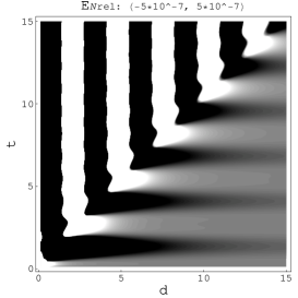
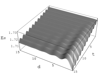
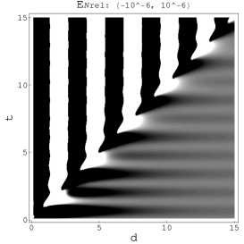
Figure 7: The early-time evolution of $E_{\cal N}$ with the first-order mutual influence included for different initial states of the detectors with $1/8<d<15$. (Upper row) All parameters are the same as those in Fig. 1 where $(\alpha,\beta)=(1.1,4.5)$ and the initial state of the detectors is entangled. Compared with Fig. 1, one can see that the distortion of the interference pattern due to the mutual influences is tiny. (Lower row) $(\alpha,\beta)=(1.5,0.2)$, the detectors also initially entangled. The distortion by the mutual influences is also tiny. As indicated by Eq. $(\ref{ENrel})$, the complicated structure of $E_{{\cal N}{\rm rel}}$ outside the light cone is reducing to simple oscillations as time goes larger.

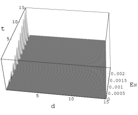
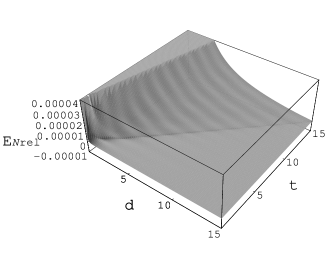
Figure 8: The early-time evolution of $E_{\cal N}$ for an initially separable detector pair with the first-order mutual influence included. The parameters are the same as those in Fig. 1 except $(\alpha,\beta)=(1,1)$ and $1/15<d<15$ here. From the left plot, one finds that quantum entanglement is created at small $d$ due to the mutual influences. In the right plot, one can see that there is no clear interference pattern in $d$ similar to those in Fig. 1 for $E_{{\cal N}{\rm rel}}$ inside the light cone. Note that here $E_{{\cal N}{\rm rel}}\equiv-\log_{2}2c_{-}(t,d)+\log_{2}2c_{-}(t,\infty)$ instead of $E_{\cal N}(t,d)-E_{\cal N}(t,\infty)$. The detectors with smaller separation $d$ always get a greater value of $-\log_{2}2c_{-}$. While there are small oscillations outside the light cone, the smaller separation $d$ always associates the greater value of $E_{{\cal N}{\rm rel}}$. The amplitude of the small oscillation is the same order of $\gamma^{2}\Lambda_{0}$ and $\gamma^{2}\Lambda_{1}$.

In the weak-coupling limit, the cross correlators $\left<\right.{\cal R}_{A},{\cal R}^{\prime}_{B}\left.\right>$ with ${\cal R},{\cal R}^{\prime}=Q,P$ are small until one detector enters the other’s light cone. From this observation one might conclude that the cross correlations between the two detectors are mainly generated by the mutual influences sourced by the quantum state of the detectors and mediated by the field. This is not always true.

As shown in Sec.V.1, the interference pattern inside the light cone has been there in the zeroth-order results, where the mutual interferences on the mode functions are not included. A comparison of the first-order results in the upper plots in Fig. 7 and those of the zeroth-order in Fig. 1 shows that the corrections to entanglement dynamics from mutual influences at early times are pretty small in that case. Actually the early-time dynamics of entanglement in both examples in Fig. 7 are dominated by the zeroth-order results, thus by the phase difference of vacuum fluctuations in $\left<\right.{\cal R}_{A},{\cal R}^{\prime}_{B}\left.\right>_{\rm v}^{(0)}$ rather than mutual influences. One can see this explicitly by inserting the mode functions in the weak-coupling limit with the first-order correction from the mutual influences into Eq.(25) in Ref. LCH08 , and write

$$\Sigma(t)\approx\Sigma_{0}+\sigma_{1}^{(0)}t+\sigma_{2}^{(0)}t^{2}+\theta(t-d)\left[\sigma_{1}^{(1)}(t-d)+\sigma_{2}^{(1)}(t-d)^{2}\right]+O(\gamma^{3})$$ (92)

at early times when $O(e^{-\gamma_{e}-(\Lambda_{0}/2)}/\Omega)<t\ll O(1/\gamma\Lambda_{i})$, $i=0,1$. Here $\Sigma_{0}$, $\sigma_{1}$, and $\sigma_{2}$ depend on $\alpha$, $\beta$ and of $O(\gamma^{0})$, $O(\gamma)$, and $O(\gamma^{2})$, respectively. Then it is easy to verify that mutual influences are negligible in the dominating $\sigma_{1}^{(1)}$ term after $\theta(t-d)$ for the initial states with the value of $\beta^{2}$ not in the vicinity of $\hbar^{2}/\alpha^{2}$ or $\alpha^{2}\Omega^{2}$.

In contrast, if the initial state (2) is nearly separable ($\beta^{2}\approx\hbar^{2}/\alpha^{2}$), mutual influences will be important in the detectors’ early-time behavior. In this case, dropping all terms with small oscillations in time, the factors in $(\ref{earlySig})$ are approximately

$$\Sigma_{0} \approx {\hbar^{2}\over 4\pi^{2}\alpha^{4}\Omega^{4}}\left[\hbar^{2}\gamma\Lambda_{1}+\alpha^{4}\Omega^{2}\gamma(2\Lambda_{0}+\Lambda_{1})\right]^{2},$$

$$\sigma_{2}^{(0)} \approx {\gamma^{2}\hbar^{2}\left(\hbar-\alpha^{2}\Omega\right)^{4}\over 4\Omega^{2}\alpha^{4}},$$

$$\sigma_{2}^{(1)} \approx -{\gamma^{2}\hbar^{2}\left(\hbar^{2}-\alpha^{4}\Omega^{2}\right)^{2}\over 4\Omega^{4}\alpha^{4}d^{2}},$$

$$\sigma_{1}^{(0)} \approx {\gamma\hbar^{2}\over 2\pi\Omega^{3}}\left[2\Omega^{2}\gamma\Lambda_{0}+\left({\hbar^{2}\over\alpha^{4}}+\Omega^{2}\right)\gamma\Lambda_{1}\right]\left(\hbar-\alpha^{2}\Omega\right)^{2},$$ (93)

with $\sigma_{1}^{(1)}$ negligible. So $\Sigma$ evolves as the following. In a very short-time scale $O(e^{-\gamma_{e}-(\Lambda_{0}/2)}/\Omega)$ after the interaction is switched on, $\Sigma$ jumps from its initial value $(\approx 0)$ to a value of the same order of $\Sigma_{0}$, which is positive and determined by the numbers $\Lambda_{0}$ and $\Lambda_{1}$ corresponding to the cutoffs of this model (the difference from the exact value is due to the oscillating terms dropped). For $\alpha^{2}\not=\hbar/\Omega$ so $Q_{A}$ and $Q_{B}$ are each in a squeezed state initially, the detectors keep separable at $t\leq d$ since $\sigma_{1}^{(0)}$ and $\sigma_{2}^{(0)}$ are positive definite. But $\sigma_{2}^{(1)}$ is negative and proportional to $1/d^{2}$, thus after entering the light cone of the other detector, if the separation $d$ is sufficiently small, or

$$d<d_{1}\equiv{1\over\Omega}\left|\hbar+\alpha^{2}\Omega\over\hbar-\alpha^{2}\Omega\right|,$$ (94)

$\sigma_{2}^{(1)}$ can overwhelm $\sigma_{2}^{(0)}$ and alter the evolution of $\Sigma$ from concave up to concave down in time. If this happens, the quantity $\Sigma$ could become negative after a finite “entanglement time”

$$t_{ent}\approx{1\over 2}\left|\sigma_{2}^{(0)}+\sigma_{2}^{(1)}\right|^{-1}\left[\sigma_{1}^{(0)}-2\sigma_{2}^{(1)}d+\sqrt{\left(\sigma_{1}^{(0)}-2\sigma_{2}^{(1)}d\right)^{2}+4\left|\sigma_{2}^{(0)}+\sigma_{2}^{(1)}\right|\left(\Sigma_{0}+\sigma_{2}^{(1)}d^{2}\right)}\right].$$ (95)

This explains the entanglement generation at small $d$ in Fig. 8. [Note that the above prediction could fail if $t_{ent}>O(1/\gamma\Lambda_{i})$, $i=0,1$, and even for $t_{ent}<O(1/\gamma\Lambda_{i})$ the above estimate on $t_{ent}$ could have an error as large as $O(2\pi/\Omega)$ due to the dropped oscillating terms.] The first-order corrections to $\left<\right...\left.\right>_{\rm a}$ contribute the $\sigma_{2}^{(1)}\cos^{2}\Omega d$ part of $\sigma_{2}^{(1)}=\sigma_{2}^{(1)}(\cos^{2}\Omega d+\sin^{2}\Omega d)$, so for those cases with separations small enough such that $\sin^{2}\Omega d\ll\cos^{2}\Omega d$ the early-time entanglement creations are mainly due to mutual influences of the detectors, which is causal.

$d_{1}$ in $(\ref{defd1})$ can serve as an estimate for the maximum distance that transient entanglement can be generated from a initially separable state in the weak-coupling limit, while for the detectors with the spatial separation between $d_{1}$ and $d_{ent}$ the transient entanglement generated at early times will disappear at late times.

References

- (1) S.-Y. Lin, C.-H. Chou and B. L. Hu, Phys. Rev. D 78, 125025 (2008).
- (2) T. Yu and J. H. Eberly, Phys. Rev. Lett. 93, 140404 (2004); L.Diosi, “Progressive decoherence and total environmental disentanglement”, in Irreversible Quantum Dynamics, eds. F.Benatti and R.Floreanini (Springer, Berlin, 2003) [arXiv:quant-ph/0301096].
- (3) A. Einstein, B. Podolsky and N. Rosen, Phys. Rev. 47, 777 (1935).
- (4) W. G. Unruh, Phys. Rev. A 59, 126 (1999).
- (5) S. Popescu and D. Rohrlich, “Causality and Nonlocality as Axioms for Quantum Mechanics”, in Proceedings of the symposium on Causality and Locality in Modern Physics and Astronomy: Open Questions and Possible Solutions (York University, Toronto, August 25-29, (1997). [arXiv:quant-ph/9709026].
- (6) A. Einstein, in The Born-Einstein Letters, edited by M. Born (Walker, New York, 1971).
- (7) J. S. Bell, Physics 1, 195 (1964).
- (8) C. Anastopoulos, S. Shresta and B. L. Hu, “Quantum Entanglement under Non-Markovian Dynamics of Two Qubits Interacting with a Common Electromagnetic Field” [arXiv:quant-ph/0610007].
- (9) B. L. Hu, J. P. Paz, and Y. Zhang, Phys. Rev. D 45, 2843 (1992).
- (10) E. Calzetta and B. L. Hu, Nonequilibrium Quantum Field Theory (Cambridge University Press, Cambridge, UK) Chapters 1, 5, 6.
- (11) J. D. Franson, J. Mod. Opt. 55, 2117 (2008).
- (12) Z. Ficek and R. Tanas, Phys. Rev. A 74, 024304 (2006).
- (13) K. Shiokawa, Phys. Rev. A 79, 012308 (2009).
- (14) C.-Y. Lai, J.-T. Hung, C.-Y. Mou, and P. Chen, Phys. Rev. B 77, 205419 (2008).
- (15) J. P. Paz and A. J. Roncaglia, Phys. Rev. Lett. 100, 220401 (2008).
- (16) C.-H. Chou, T. Yu and B. L. Hu, Phys. Rev. E 77, 011112 (2008).
- (17) S.-Y. Lin and B. L. Hu, Phys. Rev. D 73, 124018 (2006).
- (18) G. Vidal and R. F. Werner, Phys. Rev. A 65, 032314 (2002).
- (19) R. Simon, Phys. Rev. Lett. 84, 2726 (2000); L.-M. Duan, G. Giedke, J. I. Cirac, and P. Zoller, Phys. Rev. Lett. 84, 2722 (2000).
- (20) M. B. Plenio, Phys. Rev. Lett. 95, 090503 (2005).
- (21) S.-Y. Lin and B. L. Hu, Phys. Rev. D 76, 064008 (2007).
- (22) G. B. Arfken and H. J. Weber, Mathematical Methods for Physicists 6th Ed. (Elsevier, Amsterdam, 2005).