Testing model predictions of the cold dark matter cosmology for the sizes, colours, morphologies and luminosities of galaxies with the SDSS

Abstract

The huge size and uniformity of the Sloan Digital Sky Survey makes possible an exacting test of current models of galaxy formation. We compare the predictions of the GALFORM semi-analytical galaxy formation model for the luminosities, morphologies, colours and scale-lengths of local galaxies. GALFORM models the luminosity and size of the disk and bulge components of a galaxy, and so we can compute quantities which can be compared directly with SDSS observations, such as the Petrosian magnitude and the Sérsic index. We test the predictions of two published models set in the cold dark matter cosmology: the Baugh et al. (2005) model, which assumes a top-heavy initial mass function (IMF) in starbursts and superwind feedback, and the Bower et al. (2006) model, which uses AGN feedback and a standard IMF. The Bower et al model better reproduces the overall shape of the luminosity function, the morphology-luminosity relation and the colour bimodality observed in the SDSS data, but gives a poor match to the size-luminosity relation. The Baugh et al. model successfully predicts the size-luminosity relation for late-type galaxies. Both models fail to reproduce the sizes of bright early-type galaxies. These problems highlight the need to understand better both the role of feedback processes in determining galaxy sizes, in particular the treatment of the angular momentum of gas reheated by supernovae, and the sizes of the stellar spheroids formed by galaxy mergers and disk instabilities.

1 INTRODUCTION

There is a growing weight of evidence in support of the hierarchical paradigm for structure formation (Springel, Frenk & White, 2006). The principal process responsible for the growth of structure, gravitational instability, has been modelled extensively using large numerical simulations (e.g. Springel et al., 2005, 2008). The cold dark matter model gives an impressive fit to measurements of temperature fluctuations in the cosmic microwave background radiation (Hinshaw et al., 2008). When combined with other data, such as measurements of local large scale structure in the galaxy distribution or the Hubble diagram of type Ia supernovae, there is a dramatic shrinkage in the available range of cosmological parameter space (Percival et al., 2002; Sánchez et al., 2006; Komatsu et al., 2008). The spectacular progress made in constraining the background cosmology has allowed the focus to shift to trying to understand the evolution of the baryonic component of the Universe (Baugh, 2006).

Over the same period of time there has been a tremendous increase in the quantity and range of observational data on galaxies at different redshifts. Observations at high redshift have uncovered populations of massive, actively star forming galaxies which were already in place when the Universe was a small fraction of its current age (e.g. Smail et al., 1997; Steidel et al., 1999; Blain et al., 2002; Giavalisco, 2002). Huge surveys of the local universe made possible by advances in multifibre spectrographs allow the galaxy distribution to be dissected in numerous ways (e.g. Colless et al., 2003; Adelman-McCarthy et al., 2008). It is now possible to make robust measurements of the distribution of various intrinsic galaxy properties, such as luminosity, colour, morphology and size. The trends uncovered in these local surveys are influenced by a wide range of physical effects, such as star formation, supernova and AGN feedback, the cooling of gas and galaxy mergers, and hence provide as strict a test of galaxy formation models as that posed by the high redshift data.

In order to test current ideas about galaxy formation against observations, well developed theoretical tools are needed which can follow many complex processes concurrently. Most importantly, it is vital that the model predictions are produced in a form which can be compared as directly as possible with observations. Gas dynamic simulations typically follow galaxy formation in great detail for an individual dark matter halo (e.g. Governato et al., 2004; Okamoto et al., 2005; Governato et al., 2007) or within some small volume (e.g. Nagamine et al., 2004; Scannapieco al., 2006; Croft et al., 2008). In general, only limited output is available which can be compared directly with observations, such as, for example, estimates of galaxy luminosity. Currently the closest contact with observations is made by semi-analytical models of galaxy formation (see Baugh (2006) for a review). In their most sophisticated form, these models can make predictions for the luminosity, colour, scale-length and morphology of galaxies in a wide range of environments (e.g. Bower et al., 2006; Croton et al., 2006; Cattaneo et al., 2006; Monaco et al., 2007; Lagos, Cora & Padilla, 2008). These models necessarily have to treat the baryonic physics in a somewhat more idealized way than is done in the gas dynamic simulations. Physical processes are described using rules, some of which contain parameters whose values are set by comparing the model predictions with selected observations. As the range of data the model is compared against increases, the parameter space open to the models reduces. For example, the strength of supernova feedback (see Section 2) has an impact not only on the number of galaxies in the faint end of the luminosity function, but also on the size of galactic disks and even the morphological mix of galaxies.

Two key properties of semi-analytical models are their computational speed and modular nature. The impact of different processes on the nature of the galaxy population can be rapidly assessed by running models with different parameter choices. This makes the models ideal tools with which to interpret observational data. Any discrepancy uncovered between the model predictions and observations can help to identify physical ingredients which may either require better modelling or which may be missing altogether from the calculation. One clear example of how observations drive the development of the models is given by the recent efforts to reproduce the location and sharpness of the break in the galaxy luminosity function. With the current best fitting cosmological parameters, galaxy formation models struggled to avoid producing too many bright galaxies (Benson et al., 2003). One solution to this problem was suggested by observations showing the apparent absence of cooling flows at the centres of rich clusters (e.g. Peterson et al. 2003) which motivated the idea of taking into account the energy released by active galactic nuclei (AGN). This acts as a feedback process that heats the gas in massive haloes. The incorporation of this feedback mechanism suppresses the formation of galaxies in massive haloes, such that the right number of bright galaxies can be produced, and, furthermore, these galaxies have red colours to match those observed (Bower et al., 2006; Croton et al., 2006; Lagos, Cora & Padilla, 2008).

In this paper we test two published galaxy formation models run using the GALFORM semi-analytical model against statistics measured from the Sloan Digital Sky Survey. The Baugh et al. (2005) model (hereafter Baugh2005) invokes a “superwind” channel for supernova feedback, which ejects gas from low and intermediate mass haloes. This model assumes that stars are produced with a normal initial mass function (IMF) in quiescent disks but with a top-heavy IMF during merger-driven starbursts. The Baugh2005 model is able to reproduce the counts and redshift distribution of sub-millimetre selected galaxies, along with the abundance of Lyman-break galaxies and Lyman-$\alpha$ emitters (Le Delliou et al., 2005, 2006; Orsi et al., 2008). The Bower et al. (2006) model (hereafter referred to as Bower2006) incorporates AGN feedback, with the energy released by the accretion of mass onto the central supermassive black hole in halos with quasistatic hot gas atmospheres being responsible for stifling the cooling rate. The Bower2006 model gives a good match to the evolution of the K-band luminosity function and the inferred stellar mass function.

The paper is organized as follows. In Section 2, we outline the galaxy formation model GALFORM tested in the paper. In Section 3 we describe how some additional galaxy properties are computed from the model output; these properties are needed to compare the model predictions directly with observations of SDSS galaxies. Section 4 contains the comparisons between model predictions and SDSS data for the luminosity function, the distribution of morphological types, the colour distribution and the size distribution. In this section we also show the impact on the predictions of changing the strengths of various processes in the model. In Section 5 we present our conclusions. The appendices discuss how certain photometric properties of galaxies have changed between SDSS data releases and compare different indicators of galaxy type. Finally, we note that magnitudes are quoted on the AB system assuming a Hubble parameter of $h=H_{0}/100$ km s^-1 Mpc^-1; the cosmological parameters adopted depend on the choice of semi-analytic model as explained in Section 2.

2 GALAXY FORMATION MODEL

We use the Durham semi-analytical galaxy formation model, GALFORM, introduced by Cole et al. (2000) and developed in a series of subsequent papers (Benson et al., 2003; Baugh et al., 2005; Bower et al., 2006). The model tracks the evolution of baryons in the cosmological setting of a cold dark matter universe. The physical processes modelled include: i) the hierarchical assembly of dark matter haloes; ii) the shock heating and virialization of gas inside the gravitational potential wells of dark matter haloes; iii) the radiative cooling of the gas to form a galactic disk; iv) star formation in the cool gas; v) the heating and expulsion of cold gas through feedback processes such as stellar winds and supernovae; vi) chemical evolution of gas and stars; vii) mergers between galaxies within a common dark halo as a result of dynamical friction; viii) the evolution of the stellar populations using population synthesis models; ix) the extinction and reprocessing of starlight by dust. In this section we first give a comparison of the main features of the Baugh2005 and Bower2006 models, introducing the recipes used to model phenomena which are varied in Section 4. Similar discussions of these models can be found in Almeida et al. (2007), Almeida et al. (2008) and Gonzalez-Perez et al. (2008). In the second part of this section we review the model used to compute galaxy sizes, which was originally devised by Cole et al. (2000) and tested by these authors for galactic disks and by Almeida et al. (2007) for spheroids.

2.1 A comparison of the Baugh2005 and Bower2006 models

The Baugh2005 and Bower2006 models represent alternative models of galaxy formation. The parameters which specify the models were set by the requirement that their predictions should reproduce a subset of the available observations of local galaxies together with certain observations of high redshift galaxies. Different solutions were found due to the use of different physical ingredients, as set out below, and because different emphasis was placed on reproducing particular observations. We refer the reader to the original papers for a full description of each model; the Baugh2005 model is also described in detail in Lacey et al. (2008).

We now summarize the main differences between the two models.

• Cosmology. The Baugh2005 model adopts a $\Lambda$CDM cosmology with a present-day matter density parameter, $\Omega_{0}$=0.3, a cosmological constant, $\Omega_{\lambda}$=0.7, a baryon density, $\Omega_{b}=0.04$ and a power spectrum normalization given by $\sigma_{8}=0.93$. The Bower2006 model uses the cosmological model assumed in the Millennium simulation (Springel et al. 2005), where $\Omega_{0}$=0.25, $\Omega_{\lambda}$=0.75, $\Omega_{b}=0.045$ and $\sigma_{8}=0.9$, which are in somewhat better agreement with the constraints from the anisotropies in the cosmic microwave background and galaxy clustering on large scales (e.g. Sánchez et al. 2006).

• Halo merger trees. The Baugh2005 model uses a Monte-Carlo technique to generate merger histories for dark matter haloes, which is based on the extended Press-Schechter theory (Lacey & Cole, 1993; Cole et al., 2000). The formation and evolution of a representative sample of dark matter haloes is followed. In the Bower2006 model, the merger histories are extracted from the Millennium simulation (see Harker et al. 2006 for a description of the trees). The mass resolution of the simulation trees is $1.72\times 10^{10}h^{-1}M_{\odot}$, which is a factor of three worse than that used in the Monte-Carlo trees. By comparing the output of models using Monte-Carlo and N-body merger trees, Helly et al. (2003) found very similar predictions for bright galaxies, with differences only becoming apparent below some faint magnitude, the value of which depends on the mass resolution of the N-body trees. The resolution of the Millennium simulation yields a robust prediction for the luminosity function to around three magnitudes fainter than $L_{\star}$, which is more than adequate for the comparisons presented in this paper.

• Quiescent star formation timescale. The quiescent star formation rate in disks, $\psi$, is given by $\psi=M_{\rm gas}/\tau_{\ast}$, where $M_{\rm gas}$ is the mass of cold gas and the time-scale, $\tau_{\ast}$, is parameterized differently in the two models. In both cases, the star formation timescale is allowed to depend upon some power of the circular velocity of the disk and is multiplied by an efficiency factor. In the Baugh2005 model, the efficiency factor is assumed to be independent of redshift, whereas in the case of the Bower2006 model, this factor scales with the dynamical time of the galaxy [$\tau_{\rm dyn}$], measured at the half-mass radius of the disk. Since the typical dynamical time gets shorter with increasing redshift, the star formation timescale in the Bower2006 model is shorter at high redshift than it would be in the equivalent disk in the Baugh2005 model. This has implications for the amount of star formation in merger-triggered starbursts (or following a disk becoming dynamically unstable in the Bower2006 model - see later). In the Bower2006 model, disks at high redshift tend to be gas poor, with the gas being turned into stars on a short timescale after cooling, whereas in the Baugh2005 model, high redshift disks are gas rich.

• Initial mass function (IMF) for star formation. The Bower2006 model uses the Kennicut (1983) IMF, consistent with deductions from the solar neighbourhood, in all modes of star formation. The Baugh2005 model also adopts this IMF in quiescent star formation in galactic disks. However, in starbursts triggered by galaxy mergers, a top-heavy IMF is assumed. The yield of metals and the fraction of gas recycled per unit mass of stars formed are chosen to be consistent with the form of the IMF.

• Supernova (SN) feedback. With each episode of star formation, a mass of cold gas is reheated and ejected from the disk by supernova explosions at a rate given by:

  $$\dot{M}_{\rm eject}=(V_{\rm hot}/V_{\rm disk})^{\alpha_{\rm hot}}\psi,$$ (1)

  where $V_{\rm disk}$ is the velocity at the disk half-mass radius, and $V_{\rm hot}$ and $\alpha_{\rm hot}$ are parameters. The SN feedback is stronger in the Bower2006 model ($V_{\rm hot}=485{\rm kms}^{-1}$ and $\alpha_{\rm hot}=3.2$ compared with $V_{\rm hot}=300{\rm kms}^{-1}$ and $\alpha_{\rm hot}=2$ in the Baugh2005 model).

• AGN vs superwind feedback. Perhaps the most significant difference between models is the manner in which the formation of very massive galaxies is suppressed. In the Baugh2005 model, an additional channel or fate for gas heated by supernovae is invoked, called superwind feedback. In addition to the standard SNe feedback model described in the previous bullet point, some gas is assumed to be expelled completely from the halo due to heating by supernovae. The amount of mass ejected is taken to be a multiple of the star formation rate, multiplied by a function of the circular velocity of the halo. The superwind is most effective in removing gas from low circular velocity haloes, with the mass of gas ejected falling with increasing circular velocity. The gas expelled in the superwind is not allowed to recool, even in more massive haloes at later times in the merger history. This has the effect of reducing the cooling rate in massive haloes since these haloes have less than the universal fraction of baryons. Such winds have been observed in massive galaxies, with the inferred mass ejection rates found to be comparable to the star formation rate (e.g. Heckman et al. 1990; Pettini et al. 2001; Wilman et al. 2005). In the Bower2006 model an AGN feedback model is implemented which regulates the cooling rate, effectively switching off the supply of cold gas for star formation in quasi-static hot gas haloes. These are haloes in which the cooling time of the gas exceeds the free-fall time within the halo. The cooling flow is quenched by the energy injected into the hot halo by the central AGN. The growth of the black hole is followed using the model described by Malbon et al. (2007)

• Disk instabilities. In the Baugh2005 model the only process that leads to the formation of bulge stars is a galaxy merger. In the Bower2006 model, strongly self-gravitating disks are considered to be unstable to small perturbations, such as encounters with minor satellites or dark matter substructures. Such events can lead to the formation of a bar and eventually the disk is transformed into a bulge. The onset of instability is governed by the ratio

  $$\epsilon=\frac{V_{\rm disk}}{(GM_{\rm disk}/r_{\rm disk})^{1/2}}.$$ (2)

  Disks for which $\epsilon<\epsilon_{\rm disk}$, are considered to be unstable; in Bower2006, the threshold for unstable disks is set at $\epsilon_{\rm disk}=0.8$. Any cold gas present when the disk becomes unstable is assumed to participate in a starburst. As with starbursts triggered by galaxy mergers, a small fraction of the gas involved in the burst is accreted onto the central black hole. This is an important channel for the growth of low and intermediate mass black holes in the Bower2006 model.

• Treatment of reheated cold gas. The fate of gas reheated by supernovae is different in the two models. In the Baugh2005 model, as discussed above, there are two possible fates for the gas heated by supernovae: ejection from the disk to be reincorporated into the hot halo and ejection from the halo altogether, with no possibility of recooling at a later time. In the case of the first of these channels, the gas is added back into the hot halo when a new halo forms. This happens when the original halo has doubled in mass since its formation time. In the Bower2006 model, this timescale is instead taken to be some multiple of the dynamical time of the halo. Thus, gas can be reheated by supernovae, be added back into hot halo and cool again on a shorter timescale in the Bower2006 model than in the Baugh2005 model.

2.2 Galaxy scale-lengths

For completeness, We now review the calculation of the sizes of the disk and bulge components of galaxies used in GALFORM, to complement the discussion of the size predictions presented in Section 4. For a more detailed description we direct the reader to Cole et al (2000). In the following subsections, we outline how the scale-lengths of the disk and bulge are calculated. The scale-lengths are determined by solving for the dynamical equilibrium of the disk, bulge and dark matter together. Dark matter haloes are assumed to have a Navarro, Frenk & White (1997; NFW) density profile. The hot halo has a modified isothermal density profile with a core.

2.2.1 Disks

The size of a galactic disk is determined by the conservation of the angular momentum of the gas cooling from the halo and the application of centrifugal equilibrium. The disk is assumed to have an exponential surface density profile with half-mass radius $r_{\rm disk}$. The half-mass radius of the disk is related to the exponential scale-length, $h_{\rm D}$ by $r_{\rm disk}=1.68h_{\rm D}$.

The angular momentum of the dark matter halo is quantified by a dimensionless spin parameter which is drawn from a log-normal distribution, as suggested by measurements from high resolution N-body simulations (Cole & Lacey, 1996). This scheme is used in both models; the spin parameter of low-mass haloes can not be measured reliably from the Millennium simulation (Bett et al., 2007). Each newly formed halo in a halo merger tree is assigned a new spin parameter drawn from the distribution at random, independently of the previous value of the spin parameter.

As the halo collapses, the associated gas will shock and so be heated to approximately the virial temperature of the halo. Thereafter it will begin to cool via atomic processes. As gas cools it loses pressure support and flows to the center of the halo, where it is assumed to settle into a rotationally supported disk. The model assumes that the specific angular momentum of the cooling gas depends on the radius from which it originated, as described in Cole et al. (2000). The scale-length of the disk is dependent on the angular momentum of the halo gas which cools.

2.2.2 Bulges

Spheroids result from galaxy mergers, and in the case of the Bower2006 model also from dynamical instabilities of disks. The size of the spheroid produced by these events is calculated by considering virial equilibrium and energy conservation. We assume that the projected density profile is well described by a de Vaucouleurs $r^{1/4}$ law (e.g. Binney & Tremaine 1987). The effective radius, $r_{\rm e}$, of the $r^{1/4}$ law, i.e. the radius that contains half the mass in projection, is related to the half-mass radius in three dimensions, $r_{\rm bulge}$, by $r_{\rm bulge}=1.35r_{\rm e}$.

When dark matter haloes merge, the galaxy in the most massive halo is assumed to become the central galaxy in the new halo while the other galaxies become satellites. The orbits of the satellites gradually decay as energy and angular momentum are lost via dynamical friction. Eventually a satellite will merge with the central galaxy if the timescale for the orbit to decay is shorter than the halo lifetime.

Two types of merger are distinguished, major mergers and minor mergers, according to the ratio of the mass of the smaller galaxy to the larger galaxy $M_{2}/M_{1}$. If the ratio is $M_{2}/M_{1}\geq f_{\rm ellip}$, then a major merger is assumed to have taken place. Both stellar disks are transformed into spheroid stars and added to any pre-existing bulge. Any cold gas present takes part in a starburst. If the ratio is $M_{\rm 2}/M_{\rm 1}\leq f_{\rm ellip}$ then a minor merger is assumed and the stars of the smaller galaxy are added to the bulge of the central galaxy, which keeps its stellar disk. If $f_{\rm ellip}>M_{\rm 2}/M_{\rm 1}\geq f_{\rm burst}$ and the central galaxy is gas rich, then the minor merger may also be accompanied by a burst. The parameter $f_{\rm ellip}=0.3$ in both models; $f_{\rm burst}=0.05$ in Baugh2005 and $f_{\rm burst}=0.1$ in Bower2006. Disks are considered gas rich if 10% of the total disk mass in stars and cold gas is in the form of cold gas in Bower2006; this threshold is set higher, 75%, in Baugh2005.

In a merger, the two galaxies are assumed to spiral together until their separation equals the sum of their half-mass radii, which is the moment when they are considered to have merged. We estimate the radius of the merger remnant using energy conservation. Assuming virial equilibrium, the total internal energy $E_{\rm int}$ of each galaxy (both for the merging components and the remnant of the merger) is related to its gravitational self-binding energy $U_{\rm int}$ by $E_{\rm int}=-\frac{1}{2}U_{\rm int}$, and so can be written as

$$E_{\rm int}=-\frac{\bar{c}}{2}\frac{GM^{2}}{r},$$ (3)

where $M$ and $r$ are the mass and half-mass radius respectively and $\bar{c}$ is a form factor which depends on the distribution of mass in the galaxy. For a de Vaucouleurs profile, $\bar{c}=0.45$, while for an exponential disk, $\bar{c}=0.49$. For simplicity, in the model we assume $\bar{c}=0.5$ for all galaxies.

The orbital energy of a pair of galaxies at the moment of merging is given by

$$E_{\rm orbit}=-\frac{f_{\rm orbit}}{2}\frac{GM_{1}M_{2}}{r_{1}+r_{2}},$$ (4)

where $M_{1}$ and $M_{2}$ are the masses of the merging galaxies, $r_{1}$ and $r_{2}$ are their half-mass radii, and $f_{\rm orbit}$ is a parameter which depends on the orbital parameters of the galaxy pair. A fiducial value of $f_{\rm orbit}=1$ is adopted which corresponds to two point mass galaxies in a circular orbit with separation $r_{1}+r_{2}$. The galaxy masses $M_{1}$ and $M_{2}$ include the total stellar and cold gas masses and also some part of the dark matter halo. We assume that the mass of dark matter which participates in the galaxy merger in this way is a multiple $f_{\rm dark}$ of dark halo mass $M_{i,\rm dark}$ within the galaxy half-mass radius. We adopt a fiducial value $f_{\rm dark}=2$. We thus have:

$$M_{i}=M_{i,\rm stellar+gas}+f_{\rm dark}M_{i,\rm dark}.$$ (5)

Later on we will investigate the effect of varying $f_{\rm orbit}$ and the dark matter mass contribution $f_{\rm dark}$.

Assuming that each merging galaxy is in virial equilibrium, then their total energy equals one half of their internal energy. The conservation of energy means that:

$$E_{\rm int,new}=E_{\rm int,1}+E_{\rm int,2}+E_{\rm orbit},$$ (6)

and replacing $E_{\rm int}$ with Eq. 3 and $E_{\rm orbit}$ with Eq. 4 leads to

$$\frac{(M_{1}+M_{2})^{2}}{r_{\rm new}}=\frac{M_{1}^{2}}{r_{1}}+\frac{M_{2}^{2}}{r_{2}}+\frac{f_{\rm orbit}}{\bar{c}}\frac{M_{1}M_{2}}{r_{1}+r_{2}},$$ (7)

where $r_{\rm new}$ is the half-mass radius of the remnant immediately after the merger. These equations lead to the result that, in a merger of two identical galaxies, the half-mass radius of the new galaxy increases by a factor of $4/3$ which agrees reasonably well with the factor of 1.42 found in simulations of equal mass galaxy mergers by Barnes (1992).

In the case of a bulge produced by an unstable disk (which is only considered in the Bower2006 model), the considerations that lead to the remnant size are similar to those applied to a bulge produced by mergers, leading to:

$$\frac{\bar{c}_{\rm B}(M_{\rm disk}+M_{\rm bulge})^{2}}{r_{\rm new}} = \frac{\bar{c}_{\rm B}M_{\rm bulge}^{2}}{r_{\rm bulge}}+\frac{\bar{c}_{\rm D}M_{\rm disk}^{2}}{r_{\rm disk}}$$

$$+ {f_{\rm int}}\frac{M_{1}M_{2}}{r_{1}+r_{2}},$$

where $M_{\rm bulge}$, ${r_{\rm bulge}}$ and $M_{\rm disk}$, ${r_{\rm disk}}$ refer to the masses and half-mass radii of the bulge (if any) and disk respectively. As mentioned above, the form factors $\bar{c}_{\rm B}=0.49$ and $\bar{c}_{\rm D}=0.45$ for a bulge and disk respectively. The last term in Eq. 2.2.2 represents the gravitational interaction energy of the disk and bulge, which can be approximated for a range of $r_{\rm bulge}/r_{\rm disk}$ with $f_{\rm int}=2$.

3 DERIVED GALAXY PROPERTIES

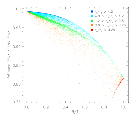
Figure 1: The ratio of Petrosian flux to total flux for a sample of GALFORM galaxies with the same selection as the SDSS, plotted as a function of the bulge to total luminosity ratio (B/T), measured in the $r-$band taking into account dust extinction. Points are colour-coded according to the ratio of disk to bulge scale-lengths, as indicated by the legend.

In this section we describe how standard GALFORM outputs, such as disk and bulge total luminosities and half-mass radii are transformed into quantities which are measured for SDSS galaxies. This allows a direct comparison between the model predictions and the observations. We outline the calculation of Petrosian magnitudes (§3.1), the concentration index (Morgan 1958; §3.2) and the Sérsic index (Sérsic, 1968). The latter two quantities are used as proxies for morphological type in analyses of SDSS data. We also illustrate how the Petrosian magnitude, concentration index and Sérsic index depend on the bulge-to-total luminosity ratio and on the ratio of the disk and bulge radii.

3.1 Petrosian magnitude

As a measure of galaxy flux, the SDSS team uses a modified definition of the Petrosian (1976) magnitude. The Petrosian radius $r_{\rm Pet}$ is defined as the radius for which the following condition holds:

$$\frac{\int_{0.8r_{\rm Pet}}^{1.25r_{\rm Pet}}{\rm d}r2\pi rI(r)/[\pi(1.25^{2}-0.8^{2})r_{\rm Pet}^{2}]}{\int_{0}^{r_{\rm Pet}}{\rm d}r2\pi rI(r)/[\pi r_{\rm Pet}^{2}]}=0.2,$$ (9)

where I(r) is the surface brightness profile. Defined in this way, $r_{\rm Pet}$ is the radius where the local surface brightness averaged within a circular annulus centred on the Petrosian radius is 0.2 times the mean surface brightness interior to that radius. The Petrosian flux defined by the SDSS is then obtained within a circular aperture of radius $2r_{\rm Pet}$. In the SDSS, the aperture used in all five bands is set by the profile of the galaxy in the r-band. I(r) is the azimuthally-averaged surface brightness measured in a series of annuli. In the case of GALFORM model galaxies, we calculate the disk and bulge sizes, and adopt an exponential profile for the disk with $I(r)\propto\exp(-1.68(r/r_{\rm D}))$, where $r_{\rm D}$ is the disk half-light radius, and a de Vaucouleurs profile for the bulge (assumed to be spherical), with $I(r)\propto\exp(-7.67(r/r_{\rm B})^{1/4})$, where $r_{\rm B}$ is the bulge half-light radius in projection (see Cole et al. 2000). The total surface brightness profile for a galaxy is given by the sum of the disk and bulge profiles. The disk and bulge magnitudes include dust extinction. A random inclination angle is assigned to the galactic disk for calculating the dust extinction. The Petrosian flux within a circular aperture of $2r_{\rm Pet}$ recovers a fraction of the total light of the galaxy which depends on its luminosity profile and hence its morphology. For a pure disk with an exponential profile, the Petrosian flux recovers in excess of 99% of the total flux. On the other hand, for a pure bulge with a de Vaucouleurs profile, the percentage of the total light recovered by the Petrosian magnitude is closer to 80%. Fig. 1 shows the ratio of Petrosian flux to total flux for model galaxies as a function the bulge-to-total luminosity ratio in the $r$-band. The limiting cases described above are apparent in the plot, which also shows the fraction of light recovered by the Petrosian definition for composite disk plus bulge systems, and for different ratios of the disk and bulge scale-lengths.

3.2 Concentration index

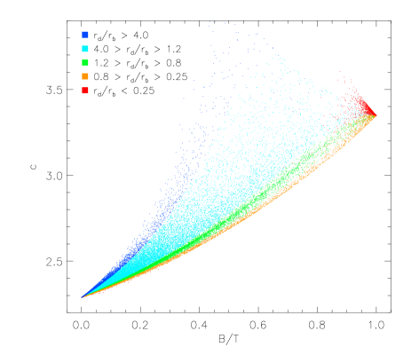
Figure 2: The concentration index, $c$, plotted as a function of the bulge-to-total luminosity (B/T) in the $r-$band for the Baugh2005 model galaxies. The ratio of disk to bulge scale-lengths is indicated by the colour of the symbol as shown by the key.

The concentration index can be straightforwardly derived once the Petrosian flux and radius have been calculated. The concentration index is defined as $c=R_{90}/R_{50}$, where $R_{90}$ and $R_{50}$ correspond to the radii enclosing $90\%$ and $50\%$ of the Petrosian flux respectively in the $r$-band. Hence, the luminosity is dominated by the bulge for high concentration galaxies and is dominated by the disk for low concentration galaxies. In Fig. 2 we plot the bulge-to-total luminosity versus the concentration index for model galaxies in the r-band. We can see that pure disks have $c=2.3$, pure bulges have $c=3.3$, and intermediate values of concentration index correspond to galaxies with different combinations of $r_{\rm disk}/r_{\rm bulge}$ and B/T. Most galaxies lie in a narrow locus of B/T versus c, but different combinations of disk and bulge scale-lengths and B/T produce the scatter shown. Observationally, the Petrosian concentration index is affected by seeing (Blanton et al., 2003a). The same galaxy can show different concentrations under different seeing conditions.

3.3 Sérsic index

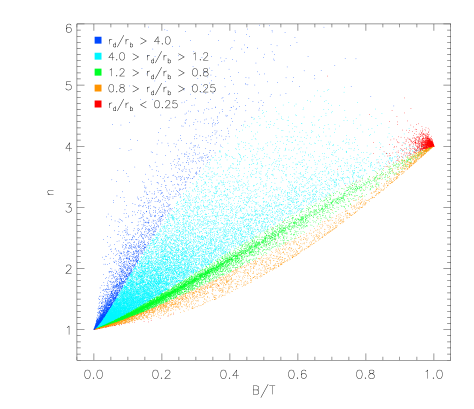
Figure 3: The Sérsic index $n$ plotted against the bulge-to-total luminosity ratio (B/T) for the Baugh2005 model galaxies. The ratio of disk to bulge scale-lengths is indicated by the colour of the symbol, as shown by the key.

The Sérsic index describes the shape of a fit made to the surface brightness profile of a galaxy without prior knowledge of the scale-lengths of the disk and bulge components. The radial dependence of the profile is given by (Sérsic 1968):

$$I(r)=I_{0}\exp[-(r/r_{0})^{1/n}].$$ (10)

Here $I_{0}$ is the central surface brightness, $r_{0}$ is the Sérsic scale radius and $n$ is the Sérsic index. The Sérsic index has been shown to correlate with morphological type (e.g. Trujillo, Graham & Caon 2001). We can see that if $n=1$ we recover an exponential profile (used for pure disk galaxies) and if $n=4$ we recover a de Vaucouleurs profile, used to describe pure bulge galaxies. The Sérsic index has been calculated in the New York University Value Added Catalogue (NYU-VAGC; Blanton et al. 2005a). Here, we do not attempt to reproduce exactly the procedure that Blanton et al. used to obtain the parameters in Eq. 10 (which takes into account seeing and pixelization). Since we know the full surface brightness profile of the model galaxies out to any radius, we want the Sérsic profile that best reproduces the composite disk plus bulge profile. In order to determine the parameters of the Sérsic profile, $I_{0}$, $r_{0}$ and $n$, we minimize a $\chi^{2}$ function which depends on the difference between the Sérsic profile and the sum of the disk and bulge surface brightness profiles, given the scale-lengths and luminosity ratio of these components:

$$\chi^{2}=\sum_{i}[\log I_{{\rm disk}+{\rm bulge}}(r_{i})-\log I_{{\rm S\acute{e}rsic}}(r_{i},r_{0},n)]^{2}W_{i}.$$ (11)

The total luminosity of the fitted Sérsic profile is constrained to be equal to that in the true disk + bulge profile. Here $r_{i}$ is a series of rings between $r=0$ to $r=R_{90,D+B}$, the radius enclosing the 90% of the disk plus bulge profile flux, and the weight $W_{i}$ is given by the luminosity in the ring containing $r_{i}$. Since the steepness of the Sérsic profile is more evident at the centre of the galaxy, we assign half of the bins to the region within the bulge size $r_{\rm bulge}$ (so as long as $r_{\rm bulge}<R_{90,D+B}$). As a test to check the consistency of changing from a disk+bulge profile to the Sérsic profile, we have compared $R_{50}$ (the radius enclosing 50% of the total luminosity) obtained from the two descriptions of the surface density profile and find very similar results.

If it is assumed that the distribution of light in real galaxies is accurately described by the Sérsic profile, then quantities derived from fitting a Sérsic profile have some advantages over the corresponding Petrosian quantities. (i) The total flux integrated over the fitted Sérsic profile would equal the true total flux, unlike the Petrosian flux, which underestimates the true total value, especially for bulge-dominated galaxies, as shown in Fig. 1. (ii) The effects of seeing can be included in the Sérsic profile fitting, so that quantities obtained from the fit (total flux, scale size $r_{0}$ and Sérsic index $n$) are in principle corrected for seeing effects, unlike the corresponding Petrosian quantities. However, since the Petrosian quantities are the standard ones used by the SDSS community, in the rest of this paper we work with Petrosian magnitude and radius, unless otherwise stated.

Fig. 3 shows the correlation between Sérsic index and the bulge-to-total luminosity ratio in the $r$-band. There is a considerable scatter between these two proxies or indicators of morphology, driven by the ratio of the scale-lengths of the disk and bulge components. For example, galaxies with a Sérsic index of $n=4$, usually interpreted as a pure bulge light profile, can have essentially any value of bulge-to-luminosity ratio from $B/T=0.1$–$1$. A key feature of this plot is the distribution of disk to bulge size ratios generated by GALFORM. It is possible to populate other parts of the $n$ - $B/T$ plane in the cases of extremely large or small values of the ratio of disk to bulge radii. Without the guidance of a physical model, if a grid of $r_{\rm d}/r_{\rm b}$ was used instead, the distribution of points would be even broader than shown in Fig. 3. Note that only model galaxies brighter than $M_{r}-5\log h=-16$ are included in this plot. A similar scatter is seen between these two quantities for real galaxies, as shown by Fig. 24 in the Appendix.

4 RESULTS

The primary observational data set we compare the model predictions against is the New York University Value Added Catalogue (NYU-VAGC), which gives additional properties to those found in the SDSS database for a subset of DR4 galaxies (Blanton et al., 2005a). The NYU catalogue covers an area of 4783 deg² and contains 49968 galaxies with redshifts. The sample is complete to $r_{\rm Pet}=17.77$ over the redshift interval $0.0033<z<0.05$, and has a median redshift of $z=0.036$. The relatively low median redshift compared with the full spectroscopic sample is designed to provide a sample of large galaxy images, suitable for measurements of galaxy morphology. Examples of the extra properties listed for galaxies, beyond the information available in the SDSS database, include the rest-frame (AB) absolute magnitude, the Sérsic index and the value of $V_{\rm max}$ (i.e. the maximum volume within which a galaxy could have been observed whilst satisfying the sample selection; this quantity is used to weight each galaxy in statistical analyses). We run GALFORM with an output redshift of $z=0.036$ to match the median of the NYU-VAGC and derive properties from the output which can be compared directly against the observations, as described in §3. In §4.1, we compare the model and observed luminosity functions, in §4.2 we show the distribution of morphological types versus luminosity, in §4.3 we examine the colour distributions and explore this further as a function of morphology in §4.4. Finally in §4.5 we test the size predictions against observations and assess the sensitivity of the model output to the strength of various processes.

4.1 Luminosity function: all galaxies and by colour

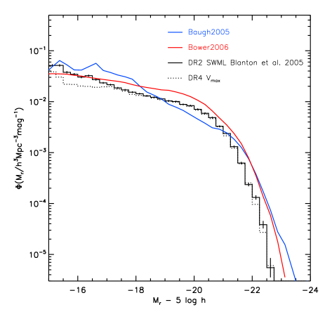
Figure 4: The $r-$band luminosity function predicted by the Bower2006 (red) and Baugh2005 (blue) models. For comparison, we also plot the SDSS luminosity function estimated using the SWML estimator by Blanton et al (2005) from DR2 (solid histogram) and our result using the $1/V_{\rm max}$ estimator from DR4 (dotted histogram).

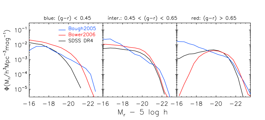
Figure 5: The colour-dependent luminosity function, for three populations of galaxies defined by the $g-r$ colour as shown by the label on top of each panel. The black lines show the luminosity function estimated from DR4 and the red (Bower2006) and blue (Baugh2005) lines show the model predictions (see the legend in the left panel).

The local luminosity function plays a key role in constraining the parameters which specify a galaxy formation model. The comparison between the predicted and observed luminosity functions is hence a fundamental test of any model. The original papers describing the Baugh2005 and Bower2006 models showed the comparison of the model predictions with the observed local luminosity function in the optical and near-infrared. However a comparison with SDSS data was not made in those papers. Fig. 4 shows the luminosity function in the Petrosian $r$-band predicted by the Baugh2005 and Bower2006 models, compared with our estimate of the luminosity function from SDSS DR4 made using the values of $V_{\rm max}$ from the NYU-VAGC catalogue. We also overplot the luminosity function estimated from the SDSS DR2 by Blanton et al. (2005b) using the stepwise maximum likelihood (SWML) method. The SWML and $1/V_{\rm max}$ estimates are in very good agreement, particularly for magnitudes brighter than $M_{r}-5\log h=-17$. At fainter magnitudes, the $1/V_{\rm max}$ estimator could be affected by very local large scale structure (Blanton et al., 2005b).

Both models overpredict the abundance of bright galaxies. The Bower2006 model produces a somewhat better match to the shape of the SDSS luminosity function. This offset in the $r-$band luminosity function has also been noted by Cai et al. (2008), who made the model galaxies in the Bower2006 model fainter by 0.15 magnitudes before using this model to make mock galaxy surveys. It is worth noting that the Bower2006 model gives an excellent match to both the $b_{\rm J}$-band luminosity function estimated from the 2dF galaxy redshift survey (Norberg et al. 2002) and to the K-band luminosity function (e.g. Cole et al. 2001; Kochanek et al. 2001) without the need to shift the model magnitudes by hand.

We can study the impact on the luminosity function of different physical processes in more detail by using colour to separate galaxies into different samples. For the SDSS data we can compute the luminosity function of colour sub-samples using the $1/V_{\rm max}$ estimator, bearing in mind that fainter than $M_{r}-5\log h=-17$ this method gives an unreliable estimate of the luminosity function due to local large-scale structure. We use the Petrosian $g-r$ colour to split galaxies into blue ($g-r<0.45$), red ($g-r>0.65$) and intermediate ($0.45<g-r<0.65$) colour samples. In Fig. 5, we can see that both models reproduce the intermediate colour population fairly well (middle panel). The Bower2006 model in particular matches the shape of the observed luminosity function closely, albeit with a shift to brighter magnitudes, similar to that seen in the case of the overall luminosity function in Fig. 4. The models fare worst for blue galaxies, with both models overpredicting the number of bright blue galaxies. This suggests that star formation is not quenched effectively enough in massive haloes or that the timescale for gas consumption in star formation is too long. For the case of red galaxies, the models do best brightwards of $L_{*}$, but get the number of faint red galaxies wrong, with the Baugh2005 model giving too many faint red galaxies and Bower2006 too few.

4.2 The distribution of morphological types

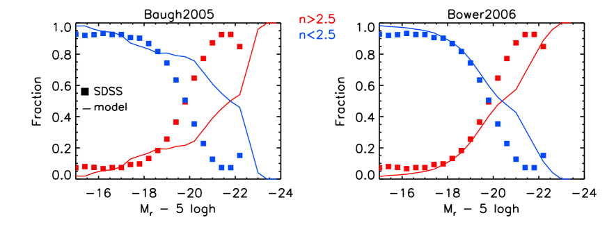
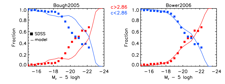
Figure 6: The fraction of different morphological types as a function of magnitude $M_{r}$ for SDSS data (squares) and GALFORM (solid lines). The fraction of disk-dominated galaxies (as defined by a value of the Sérsic index $n<2.5$) is shown in blue and bulge-dominated galaxies (i.e. those with $n>2.5$) are plotted in red. The left panel shows the Baugh2005 model and the right panel the Bower2006 model.

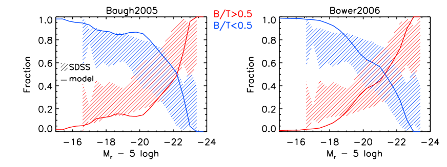
Figure 7: The fraction of different morphological types as a function of magnitude $M_{r}$ for SDSS data (squares) and GALFORM (solid lines), using the Petrosian concentration index $c$ to define type. The fraction of disk-dominated galaxies (as defined by $c<2.86$) is shown in blue and bulge-dominated galaxies (i.e. those with $c>2.86$) are plotted in red. The left panel shows the Baugh2005 model and the right panel the Bower2006 model.

Figure 8: The fraction of different morphological types as a function of magnitude $M_{r}$ using the bulge-to-total luminosity ratio in the $r-$band to define type. Disk-dominated galaxies ($B/T<0.5$) are shown in blue and bulge-dominated ($B/T>0.5$) are plotted in red. The solid curves show the model predictions, according to the label above each panel. The shaded region shows an observational estimate made from SDSS data by Benson et al. (2007). The extent of the shading shows by how much the fraction changes when a correction is applied to the observational estimates (see Benson et al. for details).

In this section we examine the mix of morphological types as a function of luminosity, using different proxies for galaxy morphology.

We first look at the mix of galaxies using the Sérsic index. Using a Sérsic index value of $n=2.5$ (which is half-way between $n=1$ and $n=4$), we separate galaxies into two broad morphological classes, disk-dominated galaxies (late type galaxies) with $n<2.5$ and bulge-dominated galaxies (early type galaxies) with $n>2.5$. Fig. 8 shows the fraction of galaxies in each morphological type, as a function of Petrosian magnitude, $M_{r}$, for SDSS galaxies and the GALFORM model (Baugh2005 in the left panel and Bower2006 in the right panel). The trend found for SDSS galaxies is that the disk-dominated population is the more common at faint magnitudes, whereas bulge-dominated objects are in the majority brighter than $L_{*}$. Fig. 8 shows that both models follow the same general trend, but with the changeover from one population to the other occuring brighter than $L_{*}$ in the Baugh2005 model, whereas the Bower2006 model looks more similar to the observations.

Another way to morphologically classify galaxies using the profile shape is to use the Petrosian concentration index $c$. In Fig. 8, we show the fraction of early and late type galaxies as a function of luminosity based on this, where we classify galaxies with $c<2.86$ as late type and $c>2.86$ as early type. The resulting plots look very similar to those based on Sérsic index in Fig. 8, though there are differences in detail, particularly at the bright end. The agreement between the models and the SDSS data is generally better using the concentration as the classifier, particularly for the Bower2006 model.

As a third approach to determining galaxy type, we consider the bulge to total luminosity ratio, $B/T$ measured in the $r-$band. Benson et al. (2007) fitted disk and bulge components to images of 8839 bright galaxies selected from the SDSS EDR. In fitting the disk and bulge components of each galaxy, they used the bulge ellipticity and disk inclination angle, $i$, as free parameters. The resulting distribution of $\cos(i)$ showed an excess of face-on galaxies. This is due in part to the algorithm mistaking part of the bulge as a disk. Benson et al. attempted to correct for the uneven distribution of inclination angles in the following way. Galaxies with $\cos(i)<0.5$ are assumed to have been correctly fitted. Since a uniform distribution in $\cos(i)$ is expected, for each galaxy with $\cos(i)<0.5$, a galaxy with a similar bulge and face-on, projected disk magnitude but with $\cos(i)>0.5$ is also selected. The galaxies with $\cos(i)>0.5$ which are left without a match are assumed to correspond to cases where the disk component has been used to fit some feature in the bulge. Benson et al. assigned to these galaxies a value of B/T=1. The correction has a considerable impact on the fraction of bulge- and disk-dominated galaxies, as shown by the extent of the shaded region in Fig. 8.

The observational estimates of the mix of morphological types presented in Figs. 8, 8 and 8 are qualitatively the same, but show that the transition from disk-dominated to bulge-dominated depends on the choice of property used to define morphology. We note that the model predictions are very similar when we set the division at $c=2.86$ or at $B/T=0.5$. The model predictions made using the Sérsic index, concentration and bulge-to-total luminosity ratio appear to be closer to each other than the corresponding observational measurements. This comparison gives some indication of the observational uncertainty in measuring fractions of different morphological types using the Sérsic index, concentration and bulge-to-total luminosity ratio.

4.3 Colour distribution

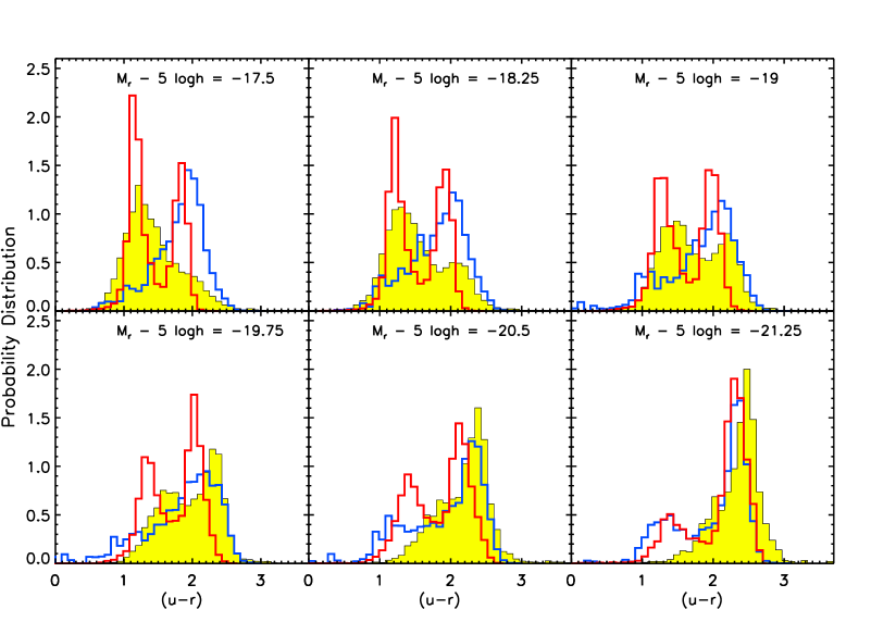
Figure 9: The $(u-r)$ colour distribution as function of luminosity for the Baugh2005 model (blue histograms), the Bower2006 model (red histograms) and the SDSS data (yellow histograms). The centre of the magnitude bin used in each panel is given by the legend. All the histograms are normalized to have unit area.

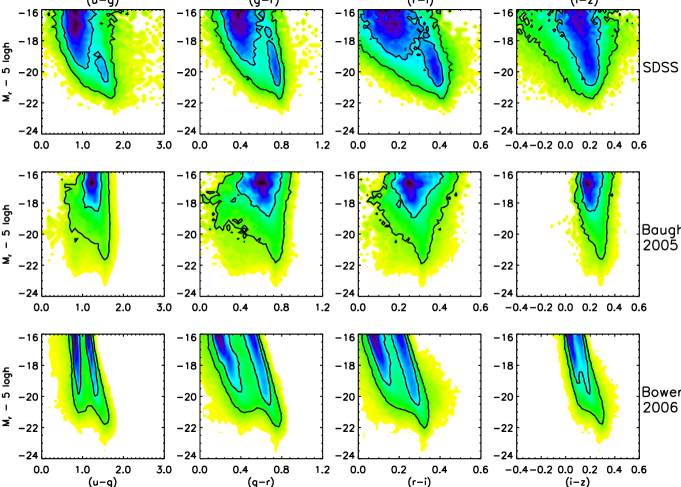
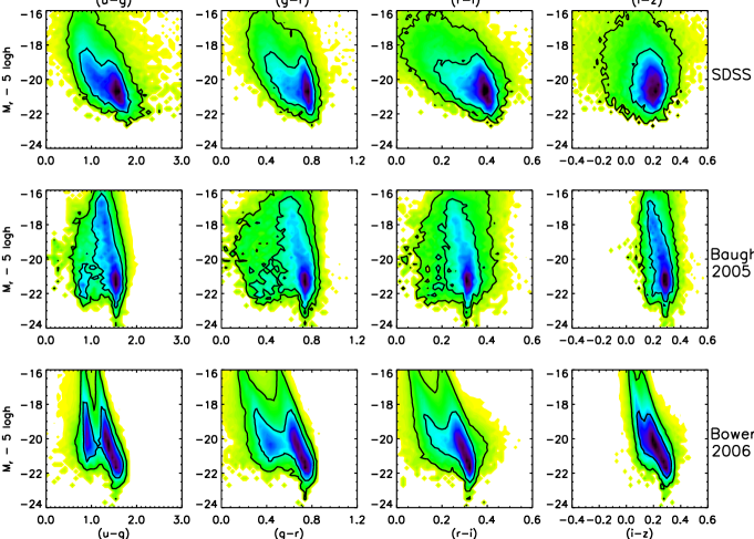
Figure 10: The galaxy distribution in the colour magnitude plane. Each column shows the distribution for a different colour. The top row shows the SDSS distributions, the middle row the predictions of the Baugh2005 model and the bottom row the Bower2006 model. Galaxies are weighted by $1/V_{\rm max}$. The inner contour encloses 68% of the total number density of galaxies and the outer contour encloses 95% of the density. The colour shading reflects the square root of the number density.

Figure 11: The same as Fig. 11, but with each galaxy weighted by the product of its luminosity and $1/V_{\rm max}$.

An important feature uncovered in the SDSS data is a bimodality in the galaxy colour-magnitude relation (e.g. Strateva et al. 2001; Baldry et al. 2004). In Fig. 9 we plot the distribution of Petrosian $(u-r)$ colour in selected bins of magnitude $M_{r}$ for models and SDSS data. The SDSS data shows a dominant red population at bright magnitudes, with a blue population that becomes more important at fainter magnitudes. Although we see blue and red populations in the Baugh2005 model predictions for intermediate magnitudes, the red population always dominates, even at the faintest magnitudes. The Bower2006 model, on the other hand displays a clear bimodality, with the red population dominating at bright magnitudes, comparable red and blue populations at intermediate magnitudes and a slightly more dominant blue population at faint magnitudes. The Bower2006 model shows the same behaviour as the SDSS data at bright magnitudes. At faint magnitudes, the Bower2006 model still shows a red population which is not apparent in the data. Font et al. (2008) argued that these faint red galaxies are predominantly satellite galaxies, which in the Bower2006 model have exhausted their cold gas reservoirs. In the Font et al. model, which is a modified version of the Bower2006 model, the stripping of hot gas from satellites is incomplete, and so gas may still cool onto the satellite, fuelling further star formation and causing these galaxies to have bluer colours on average.

Since the SDSS photometry covers five bands ($u,g,r,i$ and $z$), we can investigate the bimodality further using different colours. In Fig. 11 we plot the abundance of galaxies in the colour magnitude plane, for $(u-g),(g-r),(r-i)$ and $(i-z)$ Petrosian colours against magnitude $M_{r}$. The top row of panels shows the distributions for the NYU-VAGC SDSS data, the middle row shows the predictions of the Baugh2005 model, and the bottom row gives those of the Bower2006 model. In this plot, each galaxy contributes $1/V_{\rm max}$ to the density. The contours in the plot indicate the regions containing 68% and 95% of the number density of galaxies in the samples. Note that the colour shading scales as the square root of the density.

For the case of the SDSS data in all colours except for $(i-z)$ we can see a bright red population and a fainter, bluer population as indicated by the splitting of the 68% density contour. The Baugh2005 model predicts a dominant red population at the brightest magnitudes. On moving to fainter magnitudes, bluer galaxies appear but red galaxies still dominate and there is no clear bimodality. The Bower2006 model displays a strong bimodality in colour, though with a bluewards shift in the locus of the colour-magnitude relation compared with the observations. Font et al. (2008) obtained better agreement of their model with the observed locus of red galaxies in the SDSS by increasing the assumed yield of metals by a factor of two relative to the Bower2006 model.

In Fig. 11 we plot a similar colour-magnitude distribution, but this time each galaxy contributes $L/V_{\rm max}$ to the density. By doing this more emphasis is given to brighter galaxies. As a consequence, the bimodality in the SDSS data is less readily apparent. Intriguingly, the Baugh2005 model appears visually to be in better agreement with the observations when presented in this way.

4.4 Colour distribution by morphology

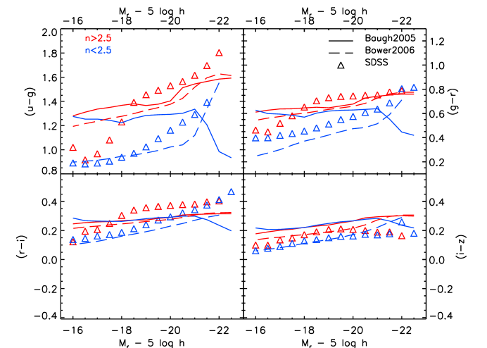
Figure 12: The median colour $(u-g),(g-r),(r-i),(i-z)$ for the models (continuous lines) and SDSS galaxies (triangles) as a function of magnitude $M_{r}$. Different coloured lines and symbols correspond to different morphological types of galaxies, as given by the Sérsic index ($n<2.5$ for the disk-dominated population and $n>2.5$ for the bulge-dominated population). Each panel corresponds to a different colour. The panels each have the same range of colour on the y-axis. The results are plotted only when there are ten or more galaxies present in a bin.

The bimodality of the colour-magnitude relation seen for SDSS galaxies suggests that different populations or types of galaxy dominate at different magnitudes. We also saw in Section 4.2 that disk-dominated galaxies are more abundant at faint magnitudes and the bulge-dominated population is more prevalent at bright magnitudes. A correlation is therefore expected between morphology, colour and luminosity. To see this effect more clearly, we use the Sérsic index, $n$, to separate galaxies into an “early-type” bulge-dominated population (with $n>2.5$) and a “late-type” disk-dominated population ($n<2.5$) and replot the colour-magnitude relation.

We calculate the median Petrosian colour for $(u-g),(g-r),(r-i),(i-z)$ in bins of magnitude $M_{r}$ for the two populations. The results are plotted in Fig. 12 for the models and the SDSS data. We can see from the SDSS data that the different populations display different colour-magnitude correlations, confirming that the Sérsic index is an effective morphological classifier. The bulge-dominated galaxies are redder than the disk-dominated galaxies, with the size of the difference decreasing as the effective wavelength of the passbands increases. Also, at fainter magnitudes, the colours of the two population tend to become more similar.

In the Baugh2005 model, Fig. 12 shows that the populations split by Sérsic index have similar colours except for the brightest galaxies. Both populations are predicted to be too red at faint magnitudes. At brighter magnitudes ($M_{r}-5\log h<-19$), bulge-dominated galaxies show similar behaviour to the SDSS data. Disk-dominated galaxies become bluer at the brightest magnitudes, which is opposite to the trend seen in the data. The Bower2006 model predicts a clear separation in colour for populations classified by Sérsic index, with blue disk-dominated galaxies even at faint magnitudes, which is in better agreement with SDSS data. In both models, the faint bulge-dominated population is predicted to be too red.

4.4.1 What drives the colours? A look at the specific star formation rate and metallicity

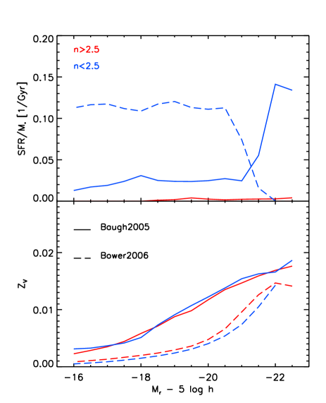
Figure 13: The top panel shows the specific star formation rate, i.e. the star formation rate per unit stellar mass, as a function of magnitude $M_{r}$ for the GALFORM models, as indicated by the key in the lower panel. The lower panel shows the stellar metallicity, weighted by the V-band luminosity as a function of magnitude $M_{r}$. Different colours correspond to different morphological types as set by the Sérsic index, as shown by the label in the top panel.

To identify which feature of the models is producing the differences in colour seen in Fig. 12, we now examine the specific star formation rate SSFR (the star formation rate [SFR] per unit stellar mass) and stellar metallicity of galaxies in both models. The specific star formation rate quantifies how vigorously a galaxy is forming stars in terms of how big a contribution recent star formation makes to the total stellar mass. Galaxies with a high specific star formation rate will tend to have bluer colours and stronger emission lines than more “passive” galaxies. We use the Sérsic index to separate the galaxies as before, into an “early-type” bulge-dominated population (with $n>2.5$) and a “late-type” disk-dominated population ($n<2.5$). In the top panel of Fig. 13 we plot the median of the SSFR as a function of magnitude $M_{r}$. In the bottom panel of this figure we plot the median of the V-band luminosity-weighted stellar metallicity. The top panel of Fig. 13 shows that bulge-dominated galaxies have very low specific star formation rates in both models. The disk-dominated galaxies have very different specific star formation rates in the two models. In the Bower2006 model, the disk-dominated galaxies are undergoing significant amounts of star formation, except at the brightest magnitudes. Although the strength of supernova feedback is stronger in the Bower2006 model than it is in the Baugh2005 model, reheated gas tends to recool on a shorter timescale because it is reincorporated into the hot halo faster. The drop in the specific star formation rate for the brightest galaxies in the Bower2006 model can be traced to the AGN feedback which shuts down gas cooling for these galaxies. Note that disk-dominated galaxies make up only a small fraction of the galaxies at these magnitudes. Within a given model, the metallicities of the disk and bulge-dominated populations are similar. However, the metallicities in the Baugh2005 model are higher than in Bower2006, presumably because some fraction of the star formation in the former model occurs in starbursts with a top-heavy IMF, which correspondingly produces a higher yield of metals. Hence, given this differences, one expects bluer galaxies at faint magnitudes in the Bower2006 model than in the Baugh2005 model.

4.4.2 Correlation between Sérsic index, colour and magnitude

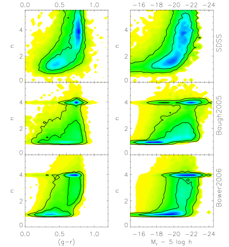
Figure 14: The luminosity-weighted density of galaxies in different projections of the Sérsic index ($n$), (g-r) colour and magnitude plane. Contours indicate the regions containing $68\%$ and $95\%$ of the total density of galaxies. Top panels: SDSS data, intermediate panels: Baugh2005 model and bottom panels: Bower2006 model.

To investigate further the correlation between the Sérsic index, colour and absolute magnitude, we plot in Fig. 14 the luminosity weighted density in the various projections of the Sérsic index ($n$), $(g-r)$ colour and $M_{i}$ absolute magnitude plane, both for SDSS data and GALFORM models. In the data we can see that disk-dominated galaxies (i.e. those with small $n$ values) tend to be bluer and also fainter, whereas the bulge-dominated galaxies (those with large $n$ values) tend to be redder and brighter. The predictions of both GALFORM models are peaked around Sérsic indices of $n=1$ (nominally pure disc galaxies) and $n=4$ (pure bulge galaxies). Despite these density peaks, the numbers of galaxies in the different morphological classes are similar to the SDSS data (as shown in Fig. 8) showing that at a broad-brush level, the distribution of $n$ predicted by the GALFORM models is in reasonable agreement with the observations.

Bearing in mind the level at which the models are able to match the distribution of Sérsic indices, both models reproduce fairly well the behaviour seen in the SDSS observation, with a spike corresponding to a faint blue disk-dominated population, which changes to a red, bulge-dominated population at bright magnitudes. Compared with the SDSS, the Baugh2005 model overpredicts the number of red disk-dominated galaxies (around values $(g-r)\sim 1$ and $n\sim 1$) and the number of moderate luminosity bulge-dominated galaxies (around values $M_{i}-5\log h\sim-19$ and $n\sim 4$). The Bower06 model predicts a distribution which agrees better with the observational data.

4.5 The distribution of disk and bulge sizes

We now examine the model predictions for the linear size of the disk and bulge components of galaxies. We compare the model predictions with SDSS observations using the radius enclosing $50\%$ of the Petrosian flux, $R_{50}$. The calculation of disk and bulge sizes was reviewed in Section 2.3 (see also Cole et al. 2000 and Almeida et al. 2007). We use the concentration index, $c$, to divide galaxies into two broad classes of disk-dominated and bulge-dominated samples. First we discuss the accuracy of the predictions for $R_{50}$ for disk-dominated galaxies (§ 4.1) and then for bulge-dominated galaxies (§ 4.2), before illustrating the sensitivity of the results to various physical ingredients of the models. The observations we compare against are our own analysis of the size distribution in the NYU-VAC constructed from DR4, as discussed below, and the results from Shen et al. (2003; hereafter Sh03), which were derived from a sample of $~{}140000$ galaxies from DR1.

4.5.1 Disk-dominated galaxies

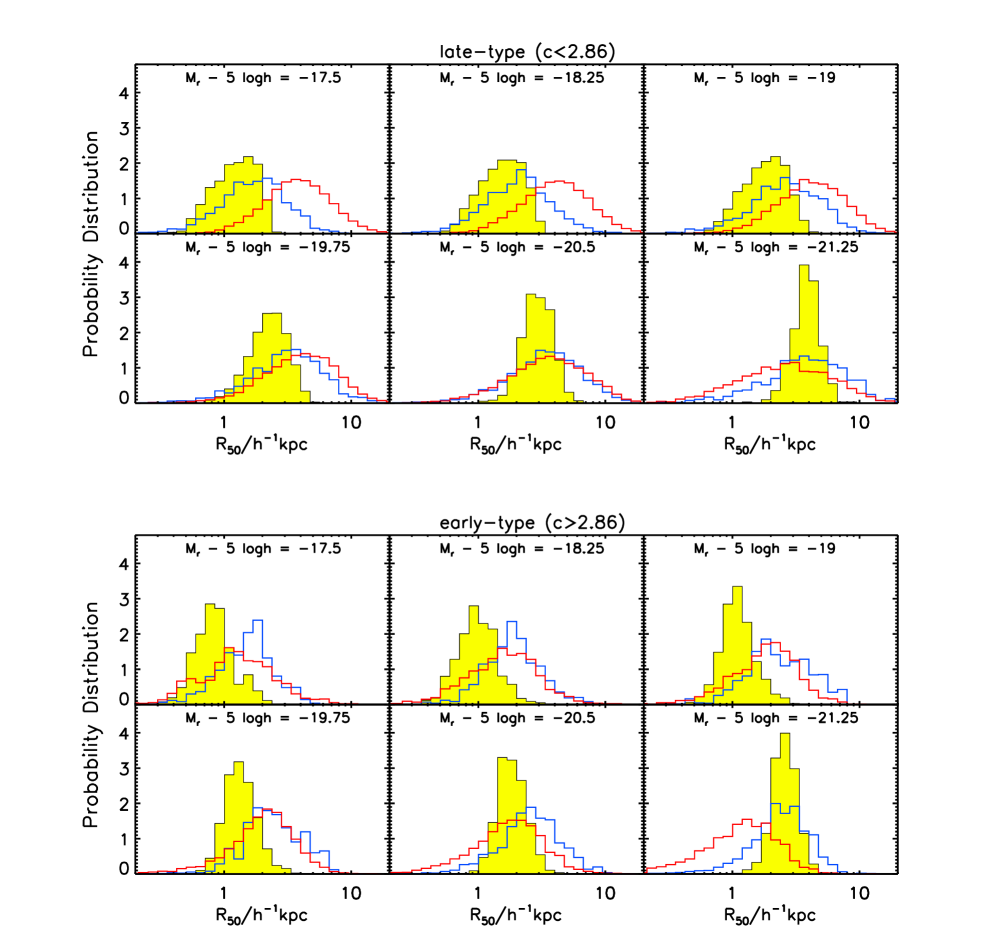
Figure 15: The distribution of the Petrosian half-light radius, $R_{50}$, for early type galaxies (with concentration parameter $c>2.86$) in top six panels and for late type galaxies ($c<2.86$) in the lower six panels. Each panel corresponds to a different one magnitude wide bin, as indicated by the legend. The GALFORM predictions are shown by unshaded histograms (Baugh2005 - blue; Bower2006 - red) and the SDSS data by the yellow shaded histogram. All of the histograms are normalized to have unit area.

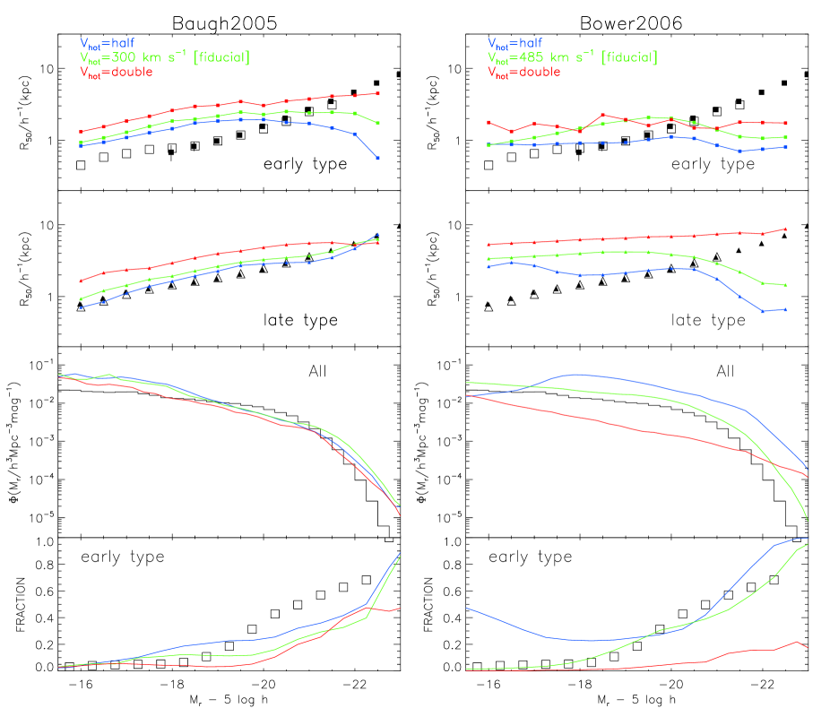
Figure 16: A compilation of predictions for the Baugh2005 (left column) and Bower2006 (right column) models. The top row shows the median $R_{50}$ as a function of magnitude for bulge-dominated galaxies ($c>2.86$), the second row shows the median $R_{50}$ for disk-dominated galaxies ($c<2.86$), the third row shows the $r-$band luminosity function of all galaxies and the bottom row shows the fraction of early-type galaxies as a function of magnitude. The predictions of the fiducial model in both cases are shown by the green lines. In this plot, we also show the impact of changing the strength of supernova feedback, rerunning the model with either half the fiducial value of $V_{\rm hot}$ (blue curves; see Section 2.1) or twice the value (red curves). In first and second rows, the open symbols show our determination of the median size from the NYU-VAGC; the filled symbols show the results obtained by Sh03. The black histogram in the third row shows our determination of the luminosity function in DR4 using the $1/V_{\rm max}$ estimator. The squares in the bottom row show the fraction of early-types in the NYU-VAGC, defined according to concentration parameter $c>2.86$, as a function of magnitude.

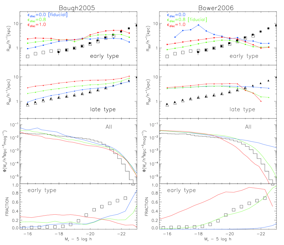
Figure 17: Similar to Fig. 16, but varying the disk instability threshold $\epsilon_{\rm disk}$ in Eq. 2.

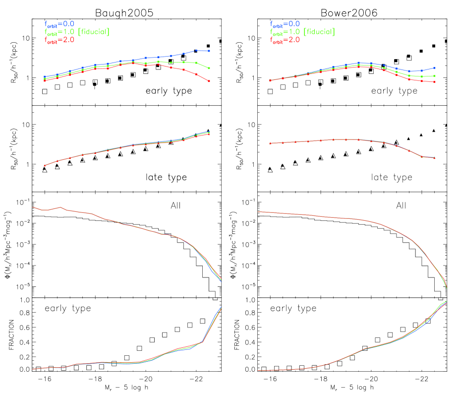
Figure 18: Similar to Fig. 16, but varying the $f_{\rm orbit}$ parameter in Eq. 7

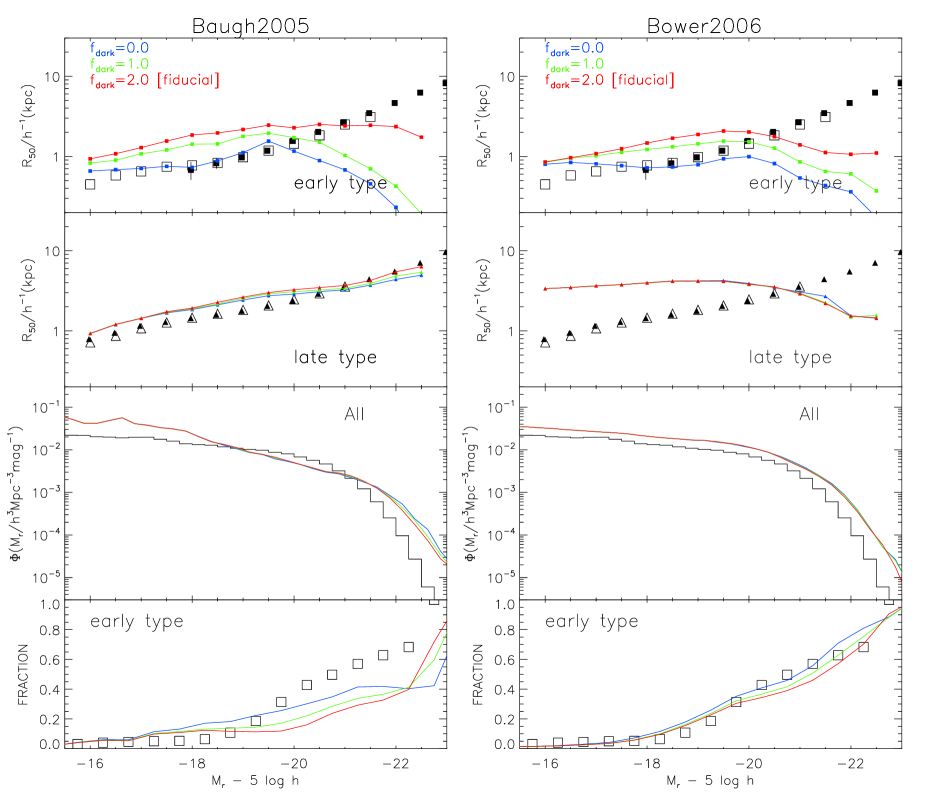
Figure 19: Similar to Fig. 16, but varying the $f_{\rm dark}$ parameter in Eq. 5

Following Sh03, we take $c<2.86$ to define the disk-dominated sample (recall that pure disk galaxies have $c\sim 2.3$ and pure bulges have $c\sim 3.3$, as shown by Fig. 2). Besides the selection introduced by use of the SDSS spectroscopic sample ($r_{\rm Pet}<17.77$), further selection criteria are required in the size distribution analysis. The size measurement for compact galaxies could be affected by the point-spread function of the image or because these objects could be misclassified as stars by the SDSS imaging processing software. To minimize such contamination, Sh03 selected galaxies with angular sizes $R_{50}>1.6^{\prime\prime}$ (this excludes only a few percent of the galaxies). Sh03 further restricted the sample to galaxies with surface brightness $\mu_{50}\leq 23.0$ mag arcsec^-2, and apparent magnitude in the range $r_{\rm min}(\theta,\phi)\leq r\leq r_{\rm max}(\theta,\phi)$ with, typically, $r_{\rm min}\sim 15.0$ and $r_{\rm max}\sim 17.77$, and redshift $z\geq 0.005$.

We apply the same criteria as used by Sh03 to the low redshift NYU-VAGC catalogue. This requires us to recalculate the value of $V_{\rm max}$ needed to construct statistical distributions, to take into account the bright magnitude limit, size cut and surface brightness cut. Note that although the Sh03 sample is from the smaller DR1, it contains more galaxies than the NYU-VAGC sample used here because it extends to higher redshift.

The correlation of size with luminosity for disk-dominated galaxies is shown in the upper six panels of Fig. 15, in which we plot the distribution of $R_{50}$ in selected magnitude bins in the $r-$band. The GALFORM predictions are plotted as unshaded histograms, with the Baugh2005 results in blue and the Bower2006 results in red. The observed distributions are shown by the yellow filled histograms. Except for the brightest two magnitude bins shown, the models tend to overpredict the size of disk-dominated galaxies, particularly in the case of the Bower2006 model. In the Baugh2005 model, the peak of the distribution shifts to larger sizes with brightening magnitude, reproducing the trend seen in the observations. On the other hand in the Bower2006 model, there is little dependence of disk size on luminosity. Both models display a larger scatter in sizes than is seen in the data. The panels for early-types are discussed in the next section.

To further quantify the trend of size with luminosity, we calculate the median value of $R_{50}$ and plot the results in Fig. 16, where the continuous green line represents the fiducial GALFORM model (the left panel shows the results for the Baugh2005 model and the right panel for the Bower2006 model) and open symbols represent the NYU-VAGC data, where we overplot for comparison (and to check for consistency) the results from Sh03 (filled triangles). Fig. 16 shows that our analysis of the size distribution in the NYU-VAGC is consistent with the results of Sh03. The apparent magnitude cut $r_{\rm min}$ together with using a low-redshift sample in comparison with Sh03, removes the galaxies brighter than $M_{r}-5\log h=-21.5$.

The SDSS data show an increase of over one decade in $R_{50}$ across the luminosity range plotted for disk-dominated galaxies. This increase is reproduced by the predictions of the Baugh2005 model. The behaviour of the Bower2006 model is quite different, with an essentially flat size-luminosity relation to $~{}L_{*}$, followed by a decrease in size for brighter galaxies. We investigate the impact of various processes on the form of the size predictions in Section 4.5.3.

4.5.2 Bulge-dominated galaxies

We select a bulge-dominated sample by taking those galaxies with concentration index $c>2.86$. In the lower six panels of Fig. 15, we plot the distribution of sizes $R_{50}$ for bulge-dominated galaxies for a selection of magnitude bins. In general, the model predicts values of $R_{50}$ larger than observed, except for the $M_{r}-5\log h=-20.5$ bin for Bower2006 and $M_{r}-5\log h=-21.25$ for Baugh2005. As for the case of disk-dominated galaxies, the predicted scatter in sizes is larger than observed.

We plot the median size of the bulge-dominated samples in the top row row of Fig. 16. The predicted size-luminosity relation is flatter than observed, turning over at the brightest magnitudes plotted. The brightest galaxies are three to five times than smaller than observed, confirming the conclusion reached by (Almeida et al., 2007).

As the DR4 data set we are working with covers a larger solid angle than the sample used by Sh03, the combined set of data measurements covers a wdier range of magnitudes than can be reached by either sample alone. Again where there is overlap, we find that our analysis of DR4 is consistent with the results of Sh03.

4.5.3 Sensitivity of the predictions to physical ingredients

The calculation of sizes involves several components as outlined in §2.2. Given that this is the area in which, overall, the model predictions agree least well with the observations, it is instructive to vary some of the physical ingredients of the model to see if the agreement can be improved. In the tests which follow, we vary the strength of one ingredient at a time and assess the impact on the size-luminosity relation. We also show the effect of the parameter change on the form of the overall galaxy luminosity function and the mix of morphological types. These variant models are not intended to be viable or alternative models of galaxy formation, but instead allow us to gain some physical insight into how the model works.

• The strength of supernova feedback.

  SN feedback plays an important role in setting the sizes of disk galaxies, by influencing in which haloes gas can remain in the cold phase to form stars. Cole et al. (2000) demonstrated that increasing the strength of SN feedback results in more gas cooling to form stars in more massive haloes, which leads to larger disks. Conversely, reducing the feedback allows gas to cool and form stars in smaller haloes resulting in smaller discs. The strength of SN feedback is parameterized using $V_{\rm hot}$ and $\alpha_{\rm hot}$ as shown in Eq. 1. The adopted values for these parameters are: $V_{\rm hot}=300\,{\rm km\,s}^{-1}$ and $\alpha_{\rm hot}=2$ in the Baugh2005 model and $V_{\rm hot}=485\,{\rm km\,s}^{-1}$ and $\alpha_{\rm hot}=3.2$ in the Bower2006 model. We perturb the models by increasing and reducing the value of $V_{\rm hot}$ to its double and half the fiducial value in each model, and plot the results in Fig. 16. The normalization of the size-luminosity relation for disk-dominated galaxies changes as expected on changing the strength of supernova feedback, moving to larger sizes on increasing $V_{\rm hot}$ and smaller sizes on reducing $V_{\rm hot}$. Reducing $V_{\rm hot}$ in the Baugh2005 model leads to better agreement with the observed size-luminosity relation for disk-dominated galaxies, at the expense of producing slightly more faint galaxies. Similar trends are seen in the predictions for the size-luminosity relation of bulge-dominated galaxies. Note that there are very few bulge-dominated galaxies at faint magnitudes in the Bower2006 model, hence the noisy size-luminosity relation in this region. Changing the strength of feedback in this way has little impact on the slope of the size-luminosity relation.

• The threshold for disks to become unstable.

  The threshold for a disk to become unstable is set by the parameter $\epsilon_{\rm disk}$ (see Eq. 2). We show the result of varying this threshold in Fig. 17. In the case of the Bower2006 model, we increase and reduce the threshold from the fiducial value of $\epsilon_{\rm disk}=0.8$; increasing the threshold means that more disks become unstable. The original Baugh2005 model does not test for the stability of disks, so in this case we switch the effect on and try two different values for the threshold. The result of turning on dynamical instabilities is straightforward to understand in this model. For a given mass and rotation speed of disk, the stability criteria $\epsilon\propto\sqrt{r_{\rm disk}}$, and so disks with smaller values of $r_{\rm disk}$ will preferentially be unstable. The removal of small disks raises the median disk size but reduces the fraction of galaxies that are disk-dominated. The impact of varying the stability threshold on the Bower2006 model is less easy to interpret: even though the fraction of faint disk-dominated galaxies fails dramatically on increasing the threshold, there is little change in the median size of the surviving disks. This change has a bigger impact on the size of bulge-dominated galaxies, with a sequence that is inverted compared with the Baugh2005 model. One result that is easily understood is the response of the luminosity function. The burst of star-formation which can accompany the transformation of a dynamically unstable disk into a bulge is an important channel for generating black hole mass in the Bower2006, as discussed in Section 2.2. If fewer disks become unstable, less mass is converted into black holes and AGN feedback has less impact on the cooling flows in massive haloes, leading to too many bright galaxies.

• The orbital energy of merging galaxies

  The parameter $f_{\rm orbit}$ quantifies the orbital energy of two galaxies which are about to merge (Eq. 4). Our standard choice in both models is $f_{\rm orbit}=1$, in which case Eq. 4 is equal to the energy of two point masses in a circular orbit at a separation of $r_{1}+r_{2}$. We vary the value of $f_{\rm orbit}$ trying $f_{\rm orbit}=0$, which corresponds to a parabolic orbit, and $f_{\rm orbit}=2$. The results are plotted in Fig. 18. As expected, the median size of disk-dominated galaxies is unaffected by varying $f_{\rm orbit}$. Increasing the value of $f_{\rm orbit}$ makes bulge-dominated galaxies smaller, with a larger effect seen for brighter galaxies. A smaller value of $f_{\rm orbit}$ improves the shape of the size-luminosity relation of bulge-dominated galaxies in the Baugh2005 model; however, faint bulge-dominated galaxies are still too large after making this change.

• The contribution of the dark matter in galaxy mergers

  The parameter $f_{\rm dark}$ controls the amount of dark matter associated with model galaxies during merger evenst (see Eq. 5), which has an impact on the size of the merger remnant, through Eq. 4 and Eq. 7. We run the models using values of $f_{\rm dark}=1$ and $f_{\rm dark}=0$, the latter of which corresponds to the case of a galaxy without participating dark matter. We can see that the reduction of $f_{\rm dark}$ from the fiducial value leads to smaller sizes for the early type galaxies in both models. The effect is particularly important at bright magnitudes. As expected, there is no change in the predicted sizes for late type galaxies. We do not find, either, a variation in the luminosity function, but there is an increase in the fraction of early type galaxies, particularly at intermediate magnitudes. We can see that we can improve the sizes of early type galaxies, matching with those inferred from SDSS observations for galaxies with magnitudes fainter than $L\star$. However, this change is counterproductive at bright magnitudes, resulting in even smaller sizes.

4.5.4 What drives the slope of the size-luminosity relation?

We have seen that the prediction of the Bower2006 model for the size-luminosity relation of disk-dominated galaxies is much flatter than that of the Baugh2005 model (Fig. 16). Moreover the Baugh2005 model is in better agreement with the observed relation. In the previous section we varied selected model parameters one at a time relative to the fiducial model, to show their impact on the model size-luminosity relation. In this exercise, the most dramatic change in the Bower2006 predictions resulted from varying the strength of SNe feedback. Reducing the value of the parameter $V_{\rm hot}$, which sets the “pivot” velocity below which SNe feedback has a strong impact, leads to a shift in the size-luminosity relation to smaller sizes, with an improved match to the observed relation recovered for intermediate luminosity galaxies. In this section, we investigate the effect of varying several parameters together, essentially moving from the Bower2006 parameters for SNe feedback and the star formation timescale in disks, towards a set which more closely resembles that used in the Baugh2005 model. The size-luminosity relations for disk- and bulge-dominated galaxies are plotted in Fig. 20 for a sequence of models. The starting point is the fiducial Bower2006 model. For each step in the sequence, one parameter is varied relative to the previous step, as shown in the key in Fig. 20. The first change made is to the value of $\alpha_{\rm hot}$, which controls the slope of the SNe feedback. Changing from the Bower2006 value of $\alpha_{\rm hot}=3.2$ to $\alpha_{\rm hot}=1$ gives a much improved match to the observed size-luminosity relation, particularly for intermediate luminosities. Faint disk-dominated galaxies are still somewhat too large, and bright galaxies in general are still too small. The next step is to retain the above change to $\alpha_{\rm hot}$, and also to change the value of $V_{\rm hot}$ to that used in Baugh2005. This results in a modest improvement in the size-luminosity relation for faint galaxies. Finally, the scaling of the quiescent star formation timescale with the disk dynamical time is switched off. The resulting size-luminosity relation is now in very good agreement with the observations for disk-dominated galaxies. However, bright bulge-dominated galaxies are still too small. Furthermore, the luminosity function and the predicted fraction of early types with luminosity are now much poorer matches to observations than in the fiducial Bower2006 model (lower two panels of Fig. 20).

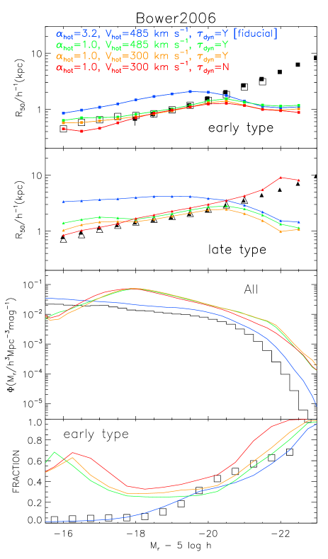
Figure 20: The impact of cumulative parameter changes for a sequence of models, starting from the fiducial model of Bower2006 (blue). One parameter is changed in each step, but unlike the cases presented in Figs. 16, 17, 18, 19, the change made is relative to the previous model in the sequence. The key lists the parameter change relative to the previous model in the sequence. The upper two panels show the size-luminosity relation for bulge and disk-dominated galaxies respectively. The third panel shows the luminosity function and the bottom panel shows the morphological mix of galaxies as a function of luminosity.

In summary, even though the sizes of disk-dominated galaxies can be brought into reasonable agreement with observations in a variant of the Bower2006 model with modified SNe feedback and disk star formation timescale, this is at the expense of agreement with the observed luminosity function and early-type fraction. Furthermore, neither the fiducial Baugh2005 model nor the fiducial or modified Bower2006 models are able to reproduce the observed sizes of early-type galaxies, in particular for bright galaxies. No single parameter change seemed able to solve the latter problem. The most promising area to explore further appears to be the modelling of galaxy mergers; changing the amount of orbital energy brought in by merging galaxies in our prescription led to an increase in the sizes of the brightest bulge-dominated galaxies.

5 SUMMARY AND DISCUSSION

Observations of local galaxies have always played a central role in setting the parameters of galaxy formation models. However, the huge size of the SDSS sample combined with the quality and uniformity of the data allow much more precise and exacting tests of the physics of such models than was previously possible. To take full advantage of this opportunity, it is necessary for the model to be able to generate predictions which are as close as possible to the measurements made for real galaxies. In this paper we use the GALFORM model, which predicts the size of both the disk and bulge components of galaxies. Hence we are able to take the model output for the luminosity and scale-lengths of a galaxy’s disk and bulge and turn these into predictions for the quantities measured for SDSS galaxies: the Petrosian magnitude, the radius containing 50% of the Petrosian flux ($R_{50}$), the concentration parameter ($c$) and the Sérsic index ($n$), the latter two quantities providing descriptions of the light profile of the galaxy.

The first major result of this work is to understand the correlation between different indicators of galaxy morphology. The concentration parameter, Sérsic index and bulge-to-total ($B/T$) luminosity ratio have all been used to divide galaxies into morphological classes (e.g Bershady et al., 2000; Hogg et al., 2004; Benson et al., 2007). The $B/T$ ratio is easy to compute theoretically, yet is perhaps the hardest of these quantities to measure observationally. Both the $c$-$B/T$ and $n$-$B/T$ planes show scatter. This can be traced to the ratio of the disk and bulge scale-lengths; galaxies with different values of this ratio occupy different loci in the $c$-$B/T$ and $n$-$B/T$ planes. The scatter is particularly large in the case of the Sérsic index $n$ versus $B/T$. The scatter would be even larger if we simply generated galaxies by hand, taking the ratio of disk and bulge scale-lengths from a grid. The scatter we find is limited by the distribution of $r_{\rm d}/r_{\rm b}$ values predicted by GALFORM.

We compared the predictions of two different versions of the GALFORM model with SDSS data: that of Baugh et al. (2005), which has a top-heavy IMF in starbursts and feedback from superwinds, and Bower et al. (2006), which has AGN feedback and a normal IMF in all modes of star formation. In the first stage of the comparison, none of the model parameters were adjusted to improve the fit to the data. The models gave reasonable matches to the total galaxy luminosity function, with the Bower et al. model giving the best overall match to the shape. The match to the luminosity function of different colour subsamples is less impressive; both models overpredict the number of bright blue galaxies and fail to match the number of red galaxies. The Bower et al. model has a strongly bimodal colour distribution, whereas the Baugh et al. model shows only weak bimodality. The Bower et al. model agrees better overall with the observed colours in SDSS, although the predicted bimodality appears somewhat too strong, and the positions of the peaks in the colour distribution do not agree exactly with what is observed.

Another clear success of the models is in predicting the correct trend of morphological type with galaxy luminosity. We used all three morphological indicators (concentration parameter, Sérsic index and bulge-to-total luminosity ratio from disk+bulge fits) to separate galaxies into disk-dominated and bulge-dominated types. In the SDSS data, the fractions of these types are found to shift from being almost completely disk-dominated at low luminosity to almost entirely bulge-dominated at high luminosity, though with differences in the detailed behaviour depending on which morphological indicator is used. Both the Baugh et al. (2005) and Bower et al. (2006) models successfully reproduce this general trend, although the Bower et al. model agrees better in detail with the observed behaviour at intermediate luminosities. Both models qualitatively reproduce the observed correlation of colour with morphology (with bulge-dominated galaxies on average being redder than disk-dominated galaxies at every luminosity), although quantitatively the Bower et al. model agrees better with the SDSS data, the Baugh et al. model predicting too many red disk-dominated galaxies.

Perhaps the most serious shortcoming of the models is in the predicted galaxy sizes. Whilst the Baugh et al. model gives a very good match to the luminosity-size relation for disks, the sizes of bulge-dominated galaxies do not match the observations. The slope of the size-luminosity relation for bulge-dominated galaxies in the Baugh et al. model matches the observations for faint galaxies, but the normalization is too high. Brighter than $L_{*}$, the predicted relation flattens, with the consequence that the brightest bulge-dominated galaxies are around a factor of three too small (see also Almeida et al. 2007). The situation is worse for the sizes predicted by the Bower et al. model; in this case the size - luminosity relation is flat for disk-dominated galaxies, while for bulge-dominated galaxies the predicted sizes at high luminosities fall even further below the observed relation than for the Baugh et al. model. We have demonstrated that a steeper slope for the size-luminosity relation for disk-dominated galaxies can be recovered in the Bower et al. model if we set some physical processes to have the same parameters as used in the Baugh et al. model. The primary improvement in the model predictions is seen on reducing the strength of SNe feedback. Also, by adjusting the star formation timescale in disks by switching off the dependence on the disk dynamical time, we can recover the observed slope of the size-luminosity relation even at high luminosities. However, this improvement in the size - luminosity relation comes at the expense of producing too many galaxies overall.

The differences between the predictions of the two models for the sizes of disk-dominated galaxies lie in the revised cooling model adopted by Bower et al. (2006), the strength of supernova feedback, the inclusion of AGN feedback and the inclusion of dynamical instabilities for disks. In the Bower et al. model, gas which is reheated by supernova feedback is reincorporated into the hot halo on a shorter timescale than in the Baugh et al. (2005) model. Neither model is able to match the observed size of bright bulge-dominated galaxies. We explore a range of processes in the models, varying the strength of supernova feedback, changing the threshold for disks to become unstable, and changing the prescription for computing the size of the stellar spheroid formed in a galaxy merger. The latter seems the most promising solution, at least in the case of the Baugh et al. model. If we neglect the orbital energy of the galaxies which are about to merge (i.e. setting the parameter $f_{\rm orbit}=0$), then the sizes of bright galaxies are in much better agreement with the observed sizes (though the faint bulge-dominated galaxies are still too large). A similar change in the predictions results from ignoring the adiabatic contraction of the dark matter halo in response to the gravity of the disk and bulge (Almeida et al., 2007).

The GALFORM model is one of the few able to make the range of predictions considered in this paper and hence to take full advantage of the constraining power of the SDSS. The model for disk sizes works well under certain conditions, albeit with too much scatter. Our analysis suggests that the problems with disk sizes and colours are connected to the treatment of gas cooling and supernova feedback, while the problems with spheroid sizes are probably due to an overly-simplified treatment of the sizes of galaxy merger remnants. The prescription used to compute the size of spheroids is in need of improvement, which will require the results of numerical simulations of galaxy mergers. This study highlights the need to make careful and detailed comparisons with observational data in order guide improvements in the treatment of physical processes in galaxy formation models.

Appendix A Changes in the photometry of SDSS galaxies from DR1 to DR4

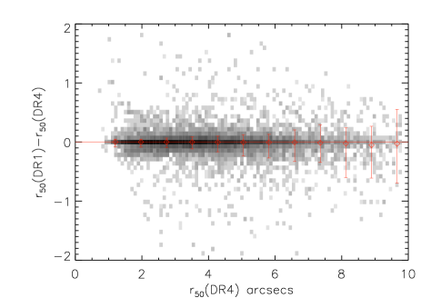
Figure 21: The difference in angular radius (in arcsec) enclosing 50% of the Petrosian magnitude, $r_{50}$, between for the same galaxies identified in DR1 and DR4. The shading reflects the logarithm of the density of galaxies. The points show the median difference in size and the bars show the 10-90 percentile range of this distribution.

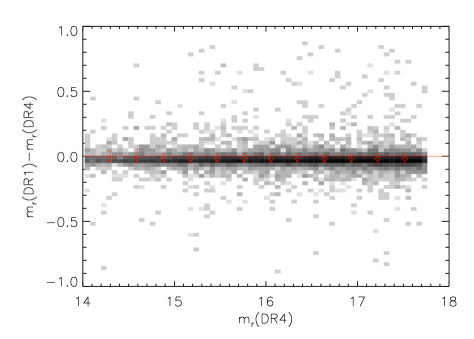
Figure 22: The difference in the Petrosian magnitude recorded in DR1 and DR4 for a matched sample of galaxies. The shading and symbols have the same meaning as in Fig. 21.

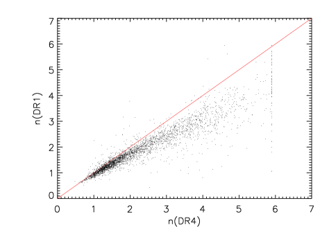
Figure 23: D The Sérsic index in DR1 plotted against that measured for the same galaxy in DR4. The shading and symbols have the same meaning as in Fig. 21.

The photometric and spectroscopic pipelines for processing SDSS data have been refined on subsequent data releases, particularly between DR1 and DR2. In DR2, all the SDSS data was re-analyzed to apply improvements to the processing of images (magnitude modelling, image deblending) and spectra (extraction of radial velocities, spectrophotometry). It is instructive to test whether any of the photometric properties used in this paper to constrain the models have changed appreciably between data releases. Uncertainty in the extraction of properties from observational data puts a limit on how well we can expect the models to reproduce the observational results. In this appendix, we compare galaxy sizes, Petrosian magnitudes and Sérsic index values between DR1 and DR4.

To perform the comparison between measurements in different data releases, we need to be sure that we are looking at the same galaxy in each version of the catalogue. This is not a trivial exercise, since revisions to the algorithm used to deblend close or merged images mean that a single object in DR1 could appear as multiple objects in DR4. The match is made by requiring that a DR4 galaxy should be closer than $1.2\arcsec$ on the sky (which is equivalent to 3 SDSS pixels, each of $0.396\arcsec$). This is close to the smallest angular size found for galaxies used in the comparison. With this criteria, we were able to find DR4 counterparts for 95% of the galaxies from DR1.

We first look at the difference in the value of angular radius enclosing 50% of the Petrosian light, which is plotted in Fig. 21 for galaxies with $z<0.05$. Here we plot the logarithm of the number density of galaxies in greyscale to expand the dynamic range of the shading. The points with error bars show the median difference in size between the two data releases, with the bars showing the 10-90 percentile range of the distribution. Although there is scatter in the sizes between data releases, there is no evidence for any systematic differences.

Next we repeat this comparison for the Petrosian magnitude, which is shown in Fig. 22 for galaxies with $z<0.05$. In this case there is a small systematic effect, with the median shift being  -0.04 mag between DR1 and DR4 i.e. a galaxy is typically brighter in DR1 and it appears in DR4.

Finally we compare the Sérsic index between DR1 and DR4. For DR1, we use the Sérsic index calculated by Blanton et al. (2003a). The analysis presented by these authors corresponds to a larger area than DR1, but relies on a pre-DR1 version of the photometric analysis software. In a subsequent publication, (Blanton et al., 2005a), the algorithm used to compute the Sérsic index was updated in order to account for a bias in the results. (Blanton et al., 2005a) demonstrated this effect by feeding a pure bulge with $n=4$ into the algorithm. With the original method, a Sérsic index of $n=2.7$ was recovered. Using the improved algorithm, the result was increased to $n=3.5$, a much smaller bias. The comparison between the Sérsic index in DR1 and DR4 is plotted in Fig. 23.The DR4 Sérsic index is generally larger than in DR1, particularly for $n>1$. The revised algorithm sometimes fails to find a suitable value for $n$, in which case $n=6$ was assigned. This comparison shows the difficulty in extracting the value of the Sérsic index for galaxies, and gives an indication of how closely we should expect the models to agree with the observational results.

Appendix B The correlation between Sérsic index and bulge to total luminosity ratio.

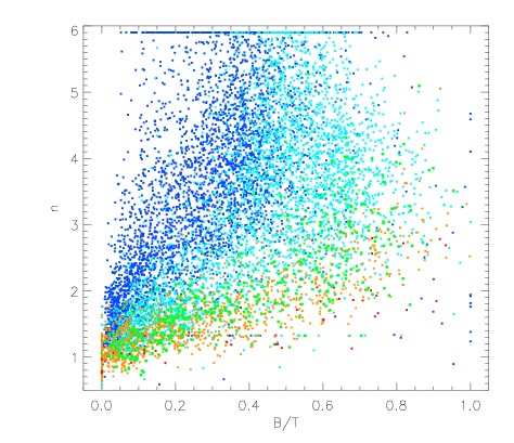
Figure 24: The Sérsic index extracted from the NYU-VAGC plotted against the bulge-to-total luminosity ratio (B/T) as determined by Benson et al. (2007). The colour coding reflects the ratio of the disk and bulge radii, which blue indicating a ratio of $r_{\rm d}/r_{\rm b}=4$ and red indicating $r_{\rm d}/r_{\rm b}=0.25$, as in Fig. 3.

In Section 3, we compared different indicators of galaxy morphology, the concentration, Sérsic index and bulge-to-total luminosity ratio using the output of GALFORM. We found considerable scatter between these quantities, particularly in the Sérsic index - bulge-to-total ratio plane. This is driven by the ratio of the disk and bulge scale-lengths; galaxies with a given ratio of scale-lengths occupy a particular locus in the plane.

We can now repeat this comparison for SDSS galaxies. Benson et al. (2007) calculated the disk and bulge radii ($r_{d}$ and $r_{b}$) and bulge-to-total luminosity ratio, $B/T$, for a sample of galaxies from the SDSS EDR. In Fig. 24 we plot the raw uncorrected values of $B/T$ found by Benson et al. (2007) against the Sérsic index $n$ for these galaxies given by the NYU-VAGC used in this paper. The galaxies are colour-coded in the same way as for the GALFORM sample plotted in Fig. 3; the largest ratio of disk to bulge radii is shown by blue points and the smallest ratio by red points. This plot looks qualitatively similar to the one obtained in Section 3 using GALFORM output, but with much more scatter. As found by Benson et al., there is a deficit of galaxies with high $B/T$.

References

- Adelman-McCarthy et al. (2008) Adelman-McCarthy J. K. et al., 2008, ApJS, 175, 297
- Almeida et al. (2007) Almeida, C., Baugh, C. M., Lacey, C. G., 2007, MNRAS, 376, 1711
- Almeida et al. (2008) Almeida C., Baugh C. M., Wake D. A., Lacey C. G., Benson A. J., Bower R. G., Pimbblet K., 2008, MNRAS, 386, 2145
- Baldry et al. (2004) Baldry I. K., Glazebrook K., Brinkmann J., Ivezic Z., Lupton R. H., Nichol R. C., Szalay A. S., 2004, ApJ, 121, 2358
- Barnes et al. (1992) Barnes J., 1992, ApJ, 393, 484
- Baugh (2006) Baugh C. M., 2006, Rep. Prog. Phys., 69, 3101
- Baugh et al. (2005) Baugh C. M., Lacey C. G., Frenk C. S., Granato G. L., Silva L., Bressan A., Benson A. J., Cole S., 2005, MNRAS, 356, 1191
- Benson et al. (2003) Benson A. J., Bower R. G., Frenk C. S., Lacey C. G., Baugh C. M., Cole S., 2003, ApJ, 599, 38
- Benson et al. (2007) Benson A. J., Dzanović D., Frenk C. S., Sharples R., 2007, MNRAS, 379, 841
- Bershady et al. (2000) Bershady, M. A., Jangren, A., & Conselice, C. J. 2000, AJ, 119, 2645
- Bett et al. (2007) Bett P., Eke V., Frenk C. S., Jenkins A., Helly J., Navarro J., 2007, MNRAS, 376, 215
- Blain et al. (2002) Blain A. W., Smail I., Ivison R. J., Kneib J.-P., Frayer D. T., 2002, Phys. Rep., 369, 111
- Blanton et al. (2001) Blanton M. R. et al., 2001, ApJ, 121, 2358
- Blanton et al. (2003a) Blanton M. R. et al., 2003, ApJ, 594, 186
- Blanton et al. (2003b) Blanton M. R., Hogg, D. W. et al., 2003, ApJ, 592, 819
- Blanton et al. (2005a) Blanton M. et al., 2005a, AJ, 129, 2562
- Blanton et al. (2005b) Blanton M. et al., 2005b, ApJ, 631, 208
- Bower et al. (2006) Bower R. G., Benson A. J., Malbon R., Helly J. C., Frenk C. S., Baugh C. M., Cole S., Lacey C. G., 2006, MNRAS, 370, 645
- Cattaneo et al. (2006) Cattaneo A., Dekel A., Devriendt J., Guiderdoni B., Blaizot J., 2006, MNRAS, 370, 165
- Colless et al. (2003) Colless M. M. et al. (the 2dFGRS Team), 2003, preprint (astro-ph/0306581)
- Cole & Lacey (1996) Cole S. & Lacey C., 1996, MNRAS, 281, 716
- Cole et al. (2000) Cole S., Lacey C. G., Baugh C. M., Frenk C. S., 2000, MNRAS, 319, 168
- Chapman et al. (2002) Chapman S. C., Scott D., Borys C., Fahlman G. G., 2002, MNRAS, 330, 92
- Croft et al. (2008) Croft R. A. C., Di Matteo T., Springel V., Hernquist L., 2008, MNRAS, submitted (arXiv:0803.4003)
- Croton et al. (2006) Croton D. J. et al., 2006, MNRAS, 367, 864
- Felten (1976) Felten, J. E., 1976, ApJ, 207, 700
- Font et al. (2008) Font, A. S., et al. 2008, MNRAS, 389, 1619
- Giavalisco (2002) Giavalisco M., 2002, ARA&A, 40, 579
- Gonzalez-Perez et al. (2008) Gonzalez-Perez, V., Baugh, C. M., Lacey, C. G., Almeida, C., 2008, MNRAS, submitted (arXiv:0811.2134)
- Governato et al. (2004) Governato F. et al., 2004, ApJ, 607, 688
- Governato et al. (2007) Governato F., Willman B., Mayer L., Brooks A., Stinson G., Valenzuela O., Wadsley J., Quinn T., 2007, MNRAS, 374, 1479
- Granato et al. (2000) Granato G. L., Lacey C. G., Silva L., Bressan A., Baugh C. M., Cole S., Frenk C. S., 2000, ApJ, 542, 710
- Harker et al. (2006) Harker G., Cole S., Helly J., Frenk C., Jenkins A., 2006, MNRAS, 367, 1039
- Heckman et al. (1990) Heckman, T. M., Armus, L., & Miley, G. K. 1990, ApJS, 74, 833
- Helly et al. (2003) Helly J. C., Cole S., Frenk C. S., Baugh C. M., Benson A. J., Lacey C. G., 2003, MNRAS, 338, 903
- Hinshaw et al. (2008) Hinshaw, G. et al., 2008, preprint (astro-ph/0803.0732)
- Hogg et al. (2004) Hogg D. W. et al., 2004, ApJ, 601, L29
- Kennicut (1983) Kennicut R. C., 1983, ApJ, 272, 54
- Komatsu et al. (2008) Komatsu, E. et al., 2008, preprint (astro-ph/0803.0547)
- Kormendy & Richstone (1995) Kormendy J., Richstone D., 1995, ARA&A, 33, 581
- Lacey & Cole (1993) Lacey C. G. & Cole S., 1993, MNRAS, 319, 627
- Lacey et al. (2008) Lacey, C. G., Baugh, C. M., Frenk, C. S., Silva, L., Granato, G. L., & Bressan, A. 2008, MNRAS, 385, 1155
- Lagos, Cora & Padilla (2008) Lagos C., Cora S., Padilla N., 2008, MNRAS, 388, 587
- Le Delliou et al. (2005) Le Delliou M., Lacey C. G., Baugh C. M., Guiderdoni B., Bacon R., Courtois H., Sousbie T., Morris S. L., 2005, MNRAS, 357, 11
- Le Delliou et al. (2006) Le Delliou M., Lacey C. G., Baugh C. M., Morris S. L., 2006, MNRAS, 365, 712
- Malbon et al. (2007) Malbon R. K., Baugh, C. M., Frenk, C. S., Lacey, C. G., 2007, MNRAS, 382, 1394
- Monaco et al. (2007) Monaco P., Fontanot F., Taffoni G., 2007, MNRAS, 375, 1189
- Morgan (1958) Morgan W. W., 1958, PASP, 70, 415
- Nagamine et al. (2004) Nagamine K., Cen R., Hernquist L., Ostriker J., Springel V., 2004, ApJ, 610, 45
- Navarro, Frenk & White (1997; NFW) Navarro J. F., Frenk C. S., White S. D. M., 1997, ApJ, 490, 493 (NFW)
- Norberg et al. (2002) Norberg P. et al., 2002, MNRAS, 336, 907
- Okamoto et al. (2005) Okamoto T., Eke V. R., Frenk C. S., Jenkins A., 2005, MNRAS, 363, 1299
- Orsi et al. (2008) Orsi, A., Lacey, C. G., Baugh, C. M., Infante, L, 2008, MNRAS, 391, 1589
- Percival et al. (2002) Percival W. J. et al., 2002, MNRAS, 337, 1068
- Perez-González et al. (2008) Perez-González P. G., Rieke G. H., Villar V. et al., 2008, ApJ, 675, 234
- Petrosian (1976) Petrosian, V., 1976, ApJ, 209, L1
- Peterson et al. (2003) Peterson J. R. et al., 2003, ApJ, 590, 207
- Pettini et al. (2001) Pettini M., Shapley A. E., Steidel C. C., Cuby J. G., Dickinson M., Moorwood A. F. M., Adelberger K. L., Giavalisco M., 2001, ApJ, 554, 981
- Sánchez et al. (2006) Sánchez A.G., Baugh C. M., Percival W. J., Peacock J. A., Padilla N. D., Cole S., Frenk C. S., Norberg P., 2006, MNRAS, 366, 189
- Scannapieco al. (2006) Scannapieco C., Tissera P. B., White S. D. M., Springel V., 2006, MNRAS, 371, 1125
- Sérsic (1968) Sérsic J. L., 1968, Atlas de Galaxias Australes, Obs. Astronómico, Córdoba
- Shen et al. (2003) Shen S., Mo H. J., White S. D. M., Blanton M. R., Kauffmann G., Voges W., Brinkmann J., Csabai I., 2003, MNRAS, 343, 978
- Smail et al. (1997) Smail I., Ivison R. J. and Blain A. W., 1997, ApJ, 490, L5
- Springel et al. (2005) Springel V., White S. D. M., Jenkins A. et al., 2005, Nat, 435, 629
- Springel, Frenk & White (2006) Springel V., Frenk C. S., White S. D. M., 2006, Nat, 440, 1137
- Springel et al. (2008) Springel. V. et al. 2008, MNRAS 391, 1685
- Steidel et al. (1996) Steidel C. C., Giavalisco M., Pettini M., Dickinson M. Adelberger K. L., 1996, ApJ, 462, 17
- Steidel et al. (1999) Steidel C., Adelberger K., Giavalisco M., Dickinson M., Pettini M., 1999, ApJ, 519, 1
- Strateva et al. (2001) Strateva V. et al., 2001, ApJ, 122, 1861
- Strauss et al. (2002) Straus M. A. et al., 2002, ApJ, 124, 1810
- Trujillo et al. (2001) Trujillo I., Graham A. W., Caon N., 2001, MNRAS, 326, 869
- Wilman et al. (2005) Wilman R. J., Gerssen J., Bower R. G., Morris S. L., Bacon R., de Zeeuw P. T., Davies R. L., 2005, Nat, 436, 227
- York et al. (2000) York D., et al, 2000, AJ, 120, 1579