A large sample study of spin relaxation and magnetometric sensitivity of paraffin-coated Cs vapor cells

Abstract

We have manufactured more than 250 nominally identical paraffin-coated Cs vapor cells (30 mm diameter bulbs) for multi-channel atomic magnetometer applications. We describe our dedicated cell characterization apparatus. For each cell we have determined the intrinsic longitudinal, $\Gamma_{\kern-1.60997pt01}$, and transverse, $\Gamma_{\kern-1.60997pt02}$, relaxation rates. Our best cell shows $\Gamma_{\kern-1.60997pt01}/2\pi\approx~{}0.5~{}\mathrm{Hz}$, and $\Gamma_{\kern-1.60997pt02}/2\pi\approx~{}2~{}\mathrm{Hz}$. We find a strong correlation of both relaxation rates which we explain in terms of reservoir and spin exchange relaxation. For each cell we have determined the optimal combination of $\mathrm{rf}$ and laser powers which yield the highest sensitivity to magnetic field changes. Out of all produced cells, 90% are found to have magnetometric sensitivities in the range of 9 to 30 $\mathrm{\mathrm{fT}}/\sqrt{\mathrm{Hz}}$. Noise analysis shows that the magnetometers operated with such cells have a sensitivity close to the fundamental photon shot noise limit.

1 Introduction

Spin polarized alkali vapors prepared by optical pumping have been used since 50 years for fundamental studies in atomic physics and applications thereof Budker:2002:RNM . The achieved sensitivities depend mainly on the (transverse) lifetime $T_{2}$ of the spin coherence in the vapor, and, to a lesser extend, on the (longitudinal) lifetime $T_{1}$ of the spin polarization. Those lifetimes are related to corresponding relaxation rates by $\Gamma_{\kern-1.60997pti}=T_{i}^{-1}$. To assure a long-lived spin polarization, the vapor cells are either filled with a buffer gas mixture or are left evacuated while applying an anti-relaxation coating on the walls. In the first case, the buffer gas in the cell confines the atoms to a diffusion-limited volume and thus reduces the rate of depolarizing wall collisions. In the second case, a thin film of paraffin or similar substance applied to the cell wall reduces the collisional sticking time with the wall and thereby the dephasing interactions with magnetic impurities embedded in the walls.

Alkali vapors in paraffin-coated cells were introduced in 1958 Robinson:1958:PSS and have since been widely applied in atomic physics spanning applications from magnetometers DiDomenico:2007:SDR ; Weis:2005:LBP ; Budker:2007:OM , over slow light studies Klein:2006:SLP , to spin-squeezing Fernholz:2008:SSA , and light-induced atomic desorption (LIAD) Alexandrov:2002:LID ; Gozzini:2008:LIS studies.

Our group develops atomic magnetometers for the accurate measurement of small changes in already weak fields (typically 10% of the earth’s field Bison:2005:OPO ), a technique that we currently apply to the measurement of the faint magnetic fields produced by the beating human heart) Bison:2003:LPM ; Weis:2006:TDR ; Hofer:2008:HSO and for magnetic field measurement and control in the search for a neutron electric dipole moment Groeger:2006:HSL ; Ban:2006:TNM . Both experiments call for a large number (50 to 100) of individual sensors to be operated simultaneously. Although buffer gas cells were used in our initial work Bison:2003:LPM , we currently focus on paraffin-coated cells that have a reduced sensitivity to magnetic field gradients because of motional narrowing and to temperature effects compared to buffer gas cells Andalkar:2002:HRM ; Vanier:1989:QPA .

In order to fulfill the requirements of the mentioned experiments we have initiated a large scale production of cells that has yielded over 250 cells in the past year. We have developed an automatic cell characterization facility for determining the quality and reproducibility of the cell coatings. In this work we describe this characterization facility in detail and report results (intrinsic relaxation times, intrinsic magnetometric sensitivity) based on significant cell statistics. A comparative study of a small sample of paraffin-coated cells produced over four decades was reported in Budker:2005:MTN . To our knowledge our present study involves the largest sample of coated cells ever compared.

2 Cell production

The paraffin-coated glass cells are manufactured in our institute. Pyrex is formed into a spherical bulb (inner diameter of $\approx 28~{}\mathrm{mm}$, wall thickness of 1 $\mathrm{mm}$) that is connected to a sidearm consisting of a Pyrex tube with 4 $\mathrm{mm}$ inner (7 $\mathrm{mm}$ outer) diameter, which acts as a reservoir to hold the droplet of solid cesium after coating, filling, and sealing the cell (Fig. 1). The metallic Cs is the source for the saturated Cs vapor filling the cell. Near the cell proper, the sidearm is constricted into a capillary with a design diameter of 0.75(25) $\mathrm{mm}$ that reduces spin depolarizing collisions with the bulk Cs in the sidearm.

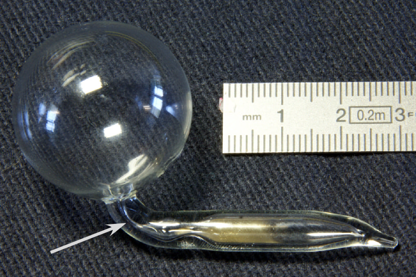
Figure 1: (Color online) Paraffin-coated Cs vapor cell. The small amount of the solid alkali metal is well visible in the sidearm. The arrow points to the capillary which reduces depolarizing collisions of vapor atoms from the cell with the solid Cs.

A typical coating and filling process takes about one week. Ten cells are mounted on a glass structure together with a paraffin containing reservoir and a Cs metal containing ampule, both isolated from the vacuum system by break-seals. The system is connected to a turbomolecular pump stand via a liquid nitrogen cold trap and all coating and filling steps are performed in a vacuum below $10^{-7}$ mbar. Prior to coating, the whole structure is baked for 5 hours at $370\,{}^{\circ}$C.

The coating process is similar to the one reported in Alexandrov:2002:LID ; Gozzini:2008:LIS . Our current choice of coating material is a commercial paraffin, Paraflint $H_{1}$, from Sasol Wax American Inc. After baking the system, the break-seal of the paraffin reservoir is broken by a piece of iron sealed in a glass bead (“hammer”) manipulated from the outside by a permanent magnet. The wax is deposited onto the cell walls by heating the paraffin reservoir. During the coating procedure the pressure rises to $9\times 10^{-7}$ mbar, and the cell is kept isolated from the cesium containing ampule. Once the cell is coated, the same hammer is used to break the seal of the Cs ampule and a thin film of metallic Cs is distilled into the cell’s sidearm by heating the Cs ampule, after which the end of the sidearm is sealed off. During Cs distillation the pressure rises to $3\times 10^{-7}$ mbar, and at the end of filling the cells are pumped down to a pressure below $10^{-7}$ mbar before being sealed. The filled cells are activated by heating them in a oven at $80\,{}^{\circ}$C for 10 hours, while assuring that the sidearm is kept at a sightly lower temperature. In this way we produce 10 coated cells in one week.

3 The cell characterization setup

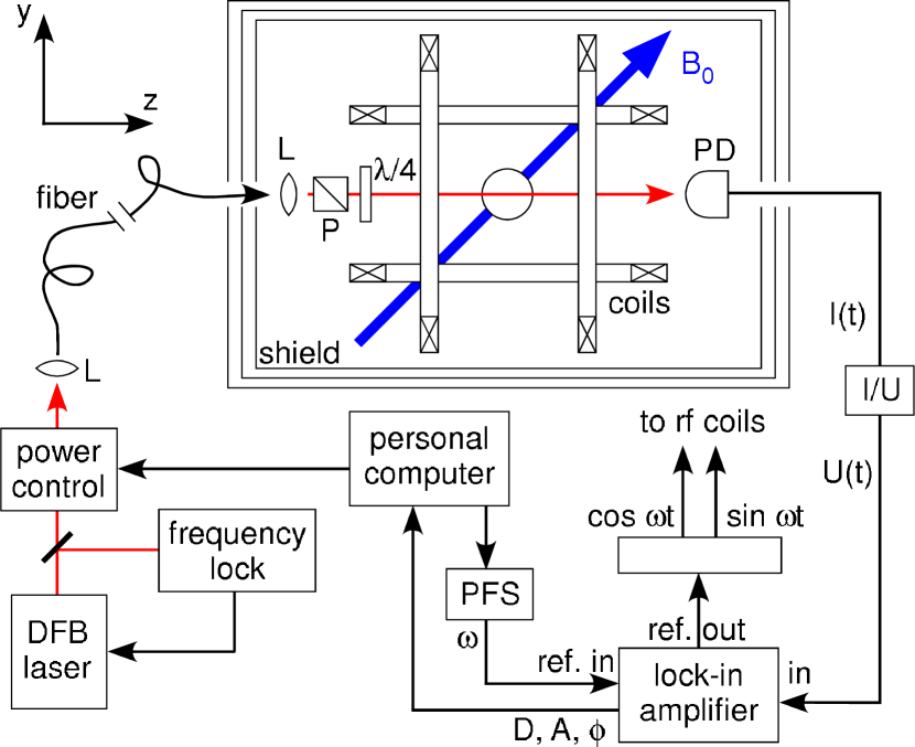
Figure 2: The cell testing apparatus. Frequency stabilized laser light is carried by a multimode fiber into a threefold magnetic shield (L: lenses). Circular polarization is created by a polarizer (P) and a quarter-wave plate ($\lambda/4$). The transmitted power is recorded by a photodiode (PD) and the modulated light power components are extracted by a lock-in amplifier. A personal computer controls the light power, performs scans of the frequency $\omega$ via a programmable frequency synthesizer (PFS, Stanford Research model SR345), and records the lock-in signals.

Following manufacture, each cell undergoes a characterization procedure in a dedicated experimental apparatus for determining the relevant parameters that indicate its magnetometric properties. Our current magnetometers use the technique of optically detected magnetic resonance in the Double Resonance Orientation Magnetometer or DROM configuration (notation introduced in Weis:2006:TDR ), also called M_x-configuration Aleksandrov:1995:LPS ; Groeger:2006:HSL . The underlying theory will be addressed below. It was thus a natural choice to use the same technique for the dedicated cell testing facility.

3.1 Experimental setup and signal recording

The experimental apparatus is shown in Fig. 2. The laser source is a DFB laser ($\lambda=894$ nm) whose frequency is actively stabilized to the $4\Rightarrow 3$ hyperfine component of the Cs $\mathrm{D}_{1}$ transition using the dichroic atomic vapor laser lock (DAVLL) technique Corwin:1998:FSD . The light is carried by a 400 $\mu\mathrm{m}$ diameter multimode fiber into a three-layer mu-metal magnetic shield that contains the actual double resonance setup. Prior to entering the fiber, the laser power, $P_{L}$, is computer-controlled via a stepper-motor driving a half-wave plate located before a linear polarizer. The light leaving the fiber is collimated and passes a linear polarizer followed by a quarter-wave plate to create circular polarization before entering the Cs cell. The fiber is wound into several loops so that the exiting light is completely depolarized, thus avoiding vibration related polarization fluctuations that translate into power fluctuations after the polarizer.

The paraffin-coated Cs cell to be characterized is placed in the center of the magnetic shields where three pairs of Helmholtz coils and three pairs of anti-Helmholtz coils compensate residual stray magnetic fields and gradients, respectively. A static magnetic field $B_{0}$ with an amplitude of a few $\mu\mathrm{T}$ is applied in the $yz$-plane at $45^{\circ}$ with respect to the laser beam direction, $\hat{k}=\hat{z}$. The transmitted light power is recorded by a nonmagnetic photodiode and then amplified. Absorbed laser light pumps the Cs atoms into the nonabsorbing (dark) $\mathinner{|{F{=}4,M_{F}{=}3,4}\rangle}$ magnetic sublevels, thereby creating a vector spin polarization (orientation) $P_{z}\propto\mathinner{\langle{F_{z}}\rangle}$. A small magnetic field $\mathrm{rf}$-field $B_{1}(t)$ of a few $\mathrm{nT}$, constant in amplitude, but rotating at frequency $\omega$, is applied in the plane perpendicular to $B_{0}$. The choice of a rotating, rather than a linearly polarized, oscillating field is used to suppress magnetic resonance transitions in the $F{=}3$ state DiDomenico:2006:ESL . $B_{1}(t)$ drives magnetic resonance transitions between adjacent sublevels in the $F{=}4$ hyperfine state, whose Zeeman degeneracy is lifted by the static magnetic field $B_{0}$. For a properly oriented magnetic field $\vec{B}_{0}$ the transmitted light power will be modulated at the rotation frequency $\omega$.

When $\omega$ is close to the Larmor frequency $\omega_{L}=\gamma_{F}B_{0}$, where $\gamma_{F}\simeq 2\pi\cdot 3.5~{}\mathrm{Hz}/\mathrm{nT}$ is the Cs ground state gyromagnetic factor, a resonance occurs in the absorption process, manifesting itself in both the amplitude and phase of the light power modulation. The corresponding in-phase, quadrature, and phase signals are extracted by means of a lock-in amplifier (LIA, Stanford Instruments, model SR830) whose output signals are read by a personal computer. The rotating field frequency is generated by a computer controlled programmable synthesizer. The computer varies this frequency, $\omega$, by a linear ramp in the range of $\pm~{}2\pi\cdot 100~{}\mathrm{Hz}$ around the Larmor frequency during a scan time of 40 s. A dedicated electronics box generates from this AC voltage two $90^{\circ}$ dephased AC currents that drive two perpendicular coil pairs (not shown in Fig. 2) producing the rotating field $B_{1}(t)$.
The characterization of each individual cell consists in the recording of resonance spectra for a set of 12 selected (and computer controlled) values of the laser power $P_{L}$ in the range of 1 to $12~{}\mu$W. It is difficult to determine the absolute laser intensity for a given laser power $P_{L}$, because of the (asymmetric) transverse beam profiles and their modification by the cell’s spherical shape. We therefore quantify the light intensity in terms of the laser power $P_{L}$, to which it is proportional. Note that $P_{L}$ used below refers to the power measured after the cell with the laser frequency resonant with the $4{\rightarrow}3$ Cs $\mathrm{D}_{1}$ transition and the $\mathrm{rf}$ power off. A typical automated characterization run, including insertion of the cell into the apparatus, takes 10 minutes. Data analysis is performed by a semi-automatic dedicated MathematicaMathematica52 code, which takes another 5 minutes. In a regular working day it is thus possible to characterize 30 to 40 cells.

3.2 DROM theory

A modulation of the transmitted power only occurs when the static magnetic field $B_{0}$ is neither parallel nor perpendicular to the direction of light propagation. In that case the transmitted light power has components that oscillate in phase, $D_{\omega}$, and in quadrature, $A_{\omega}$, with respect to the rotating field

$$B_{1}(t)=\frac{\Omega_{\mathrm{rf}}}{\gamma_{F}}\,e^{i\,\omega t}\,.$$ (1)

The in-phase and the quadrature components depend on the detuning, $\delta=\omega-\omega_{0}$, between the driving, $\omega$, and the Larmor, $\omega_{0}$, frequencies. The dependence of $D_{\omega}$ and $A_{\omega}$ on $\delta$ are dispersive and absorptive Lorentzians given by Bison:2005:OPO

$$D_{\omega}(\delta)=-\eta\mathinner{\langle{F_{z}}\rangle}\sin{(2\theta)}\frac{\Omega_{\mathrm{rf}}\delta}{\delta^{2}+\Gamma_{\kern-1.60997pt2}^{2}+\frac{\Gamma_{\kern-1.14998pt2}}{\Gamma_{\kern-1.14998pt1}}\Omega^{2}_{\mathrm{rf}}}$$

$$A_{\omega}(\delta)=-\eta\mathinner{\langle{F_{z}}\rangle}\sin{(2\theta)}\frac{\Omega_{\mathrm{rf}}\Gamma_{\kern-1.60997pt2}}{\delta^{2}+\Gamma_{\kern-1.60997pt2}^{2}+\frac{\Gamma_{\kern-1.14998pt2}}{\Gamma_{\kern-1.14998pt1}}\Omega^{2}_{\mathrm{rf}}}$$ (2)

where $A_{0}=\eta\mathinner{\langle{F_{z}}\rangle}\sin{(2\theta)}$ is a common signal amplitude that depends — via the spin polarization $\mathinner{\langle{F_{z}}\rangle}$ created by optical pumping and the detection of the polarization’s precession via light absorption — on the laser power $P_{L}$. The calibration constant $\eta$ includes all of the apparatus constants such that $D_{\omega}(\delta)$ and $A_{\omega}(\delta)$ are measured in Volts. With respect to Fig. 2, $U(t)=D_{\omega}(\delta)\cos{\omega t}+A_{\omega}(\delta)\sin{\omega t}$. The phase $\phi_{\omega}(\delta)$ between the drive and the power modulation

$$\phi_{\omega}(\delta)=+\arctan{\left(\frac{\Gamma_{\kern-1.60997pt2}}{\delta}\right)}\,,$$ (3)

depends also on the detuning $\delta$. The expressions (2) and (3) are valid for atomic media with an arbitrary ground state angular momentum, as may be shown easily by a theoretical treatment analogous to the discussion of the signals in the DRAM (double resonance alignment magnetometer) geometry presented in Weis:2006:TDR . In the above expressions, $\theta$ is the angle between the applied magnetic field $B_{0}$ and the laser beam propagation direction $\vec{k}$.

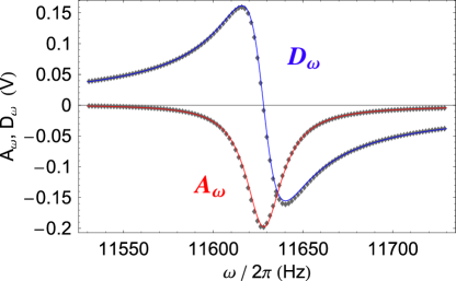
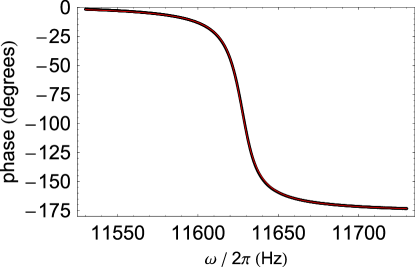
Figure 3: (color online) Lock-in demodulated magnetic resonance signals. Top: The dispersive signal (blue) represents the in-phase component $D(\omega)$ and the absorptive signal (red) the quadrature component $A(\omega)$. Bottom: Phase signal $\phi(\omega)$. Experimental points are shown together with lines fitted according to (2)–(3). All signals were recorded at $B_{0}\simeq 4~{}\mu\mathrm{T}$ ($\omega_{0}\simeq 2\pi\cdot 11640~{}\mathrm{Hz}$), with $P_{L}=6~{}\mu$W, and $B_{1}=1.3~{}\mathrm{nT}$.

3.3 Signal analysis

Since the resonance signals are extracted by a lock-in amplifier, and since it is experimentally difficult to precisely determine the phase of the rotating field (and hence the phase difference between that field and the modulation of the photocurrent), the signals produced by the lock-in amplifier are superpositions of the absorptive and dispersive lineshapes $A_{\omega}(\delta)$ and $D_{\omega}(\delta)$. Using the fitting procedure described in detail in Bison:2005:OPO it is possible to extract the pure absorptive and dispersive components. For fitting the theoretical lineshapes the combined apparatus constants $A_{0}\equiv\eta\mathinner{\langle{F_{z}}\rangle}\sin{(2\theta)}$ is taken as one fitting parameter, with $A_{0}$ measured in Volts. Other parameters are the relaxation rates $\Gamma_{\kern-1.60997pt1}$ and $\Gamma_{\kern-1.60997pt2}$, the resonance frequency $\omega_{0}$, an unknown overall phase, as well as weighting factors of the absorptive and dispersive components. The Rabi frequency $\Omega_{\mathrm{rf}}$ can be easily calibrated as described in DiDomenico:2007:SDR and a fixed numerical value is used when fitting (2) and (3).

Typical resonance lineshapes of the in-phase, quadrature, and phase signals are shown in Fig. 3, together with the fitted theoretical shapes (2) and (3). Fitting the absorptive and dispersive spectra by (2) with the relaxation rates $\Gamma_{\kern-1.60997pt1}$ and $\Gamma_{\kern-1.60997pt2}$ as free parameters yields a strong correlation between the two rates in the $\chi^{2}$-minimizing algorithm, with corresponding large uncertainties in the numerical values. We have therefore opted for the following fitting procedure. In a first step, we use the fact that the phase does not depend on $\Gamma_{\kern-1.60997pt1}$ and fit the dependence $\phi({\omega})$ given by (3) to the data. The resulting $\Gamma_{\kern-1.60997pt2}$ value is then used as a fixed parameter in the subsequent simultaneous fit of the absorptive and dispersive lineshapes to infer $\Gamma_{\kern-1.60997pt1}$. In this way we obtain $(\Gamma_{\kern-1.60997pt1},\Gamma_{\kern-1.60997pt2})$-pairs for each value of the laser power $P_{L}$. In addition, the fits yield the overall signal amplitude $A_{0}$.

Figure 4: Laser power dependence of the relaxation rates $\Gamma_{\kern-1.60997pt1}$ (boxes) and $\Gamma_{\kern-1.60997pt2}$ (diamonds). The experimental points are fitted with (4). The (statistical) error bars on the individual data points are smaller than the symbol size.

4 Results

4.1 Relaxation rates

Figure 4 shows the dependence of the longitudinal and transverse relaxation rates on the laser power $P_{L}$. There is, to our knowledge, no theoretical algebraic expression describing that dependence for ground states of arbitrary angular momentum $F$. We therefore fit, as in DiDomenico:2007:SDR , the dependence by a quadratic polynomial

$$\Gamma_{\kern-1.60997pti}(P_{L})=\Gamma_{\kern-1.60997pt0i}+\alpha_{i}\,P_{L}+\beta_{i}\,P_{L}^{2}\,,$$ (4)

which allows us to infer the intrinsic relaxation rates, $\Gamma_{\kern-1.60997pt01}$ and $\Gamma_{\kern-1.60997pt02}$, i.e., the relaxation rates extrapolated to zero light power.

Figure 5: Magnetic resonance amplitude versus laser power. The experimental points are fitted with the polynomial expression from (5), which yields, for this specific cell, the saturation parameters $P_{S1}=634$ nW and $P_{S2}=16.3~{}\mu$W. The error bars are smaller than the plotting symbol size.

4.2 Signal amplitudes

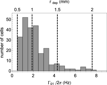
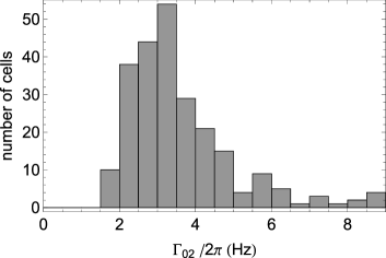
Figure 6: Histogram of intrinsic longitudinal (top) and transverse (middle) relaxation times of 241 coated cells. The upper axis in the top graph gives the radius of the effective depolarization spot that models reservoir relaxation (see text). The lower graph shows the correlation between the relaxation rates, together with a fit of the form $\Gamma_{\kern-1.60997pt02}=s\Gamma_{\kern-1.60997pt01}+a$.

Figure 5 shows the dependence of the signal amplitude $A_{0}$ on the laser power $P_{L}$. Here again, we have no theoretically derived algebraic expression describing that dependence for transitions between states with arbitrary angular momenta. We therefore, as in DiDomenico:2007:SDR , fit the experimental dependence by the empirical saturation formula

$$S_{0}(P_{L})=C\,\frac{P_{L}^{2}}{(P_{L}+P_{S1})(P_{L}+P_{S2})}$$ (5)

which accounts for an amplitude growing as $P_{L}^{2}$ at low powers, and where $P_{S1}$ and $P_{S2}$ are saturation powers.

Figures. 4 and 5 show typical dependencies of $\Gamma_{\kern-1.60997pt1}$, $\Gamma_{\kern-1.60997pt2}$, and $S_{0}$ on $P_{L}$ for a given cell, together with the fits (solid lines) by (5). We have characterized 253 paraffin-coated cells of equal diameter using the method described above. The histograms in Fig. 6 (top, middle) show the distributions of the intrinsic longitudinal and transverse relaxation rates of the 241 best cells. The scatter plot in the lower graph of Fig. 6 shows that the two rates are strongly correlated. The fitted line represents a linear relation of the form $\Gamma_{\kern-1.60997pt02}=s\,\Gamma_{\kern-1.60997pt01}+a$ with $s=1.00(1)$ and $a=1.35(3)~{}\mathrm{Hz}{}$. The longitudinal and transverse relaxation rates are thus equal, up to a constant offset that affects the $\Gamma_{\kern-1.60997pt02}$ values only. For an isotropic relaxation process, in which all Zeeman sublevels relax at the same rate, one would expect $\Gamma_{\kern-1.60997pt01}=\Gamma_{\kern-1.60997pt02}$. In section 5 below we will come back to a quantitative discussion of those contributions.

4.3 Magnetometric sensitivity

The intrinsic relaxation rates are well suited to characterize each individual cell. In particular, the transverse rate $\Gamma_{\kern-1.60997pt02}$, which determines the intrinsic width of the signals $A_{\omega}$ and $D_{\omega}$, is relevant for magnetometric applications. However, the intrinsic rates are, by definition, rates for vanishing laser and $\mathrm{rf}$ powers. Therefore, the magnetometric sensitivity of a given cell can not be inferred directly from the intrinsic rates, since magnetometers have to be operated at finite laser and $\mathrm{rf}$ power levels.

The linear zero crossing of the dispersive signal $D_{\omega}$ near resonance is convenient for magnetometric applications since any magnetic field change $\delta B$ yields a signal change

$$\delta D_{\omega}=\left|\frac{dD_{\omega}}{dB}|_{\omega{=}\omega_{L}}\right|\,\delta B$$ (6)

that is proportional to $\delta B$. The lowest magnetic field change $\delta B$ that can be detected depends on the shot noise of the DC photocurrent $I_{L}\propto P_{L}$. A feedback resistor, $R_{F}$, in the transimpedance amplifier, marked $I/U$ in Fig. 2, transforms that photocurrent into a photovoltage $U_{L}$, whose shot noise (in a bandwidth of 1 $\mathrm{Hz}$) is given by

$$\delta U_{L}=R_{F}\,\delta I_{L}=R_{F}\,\sqrt{2eI_{L}}=R_{F}\,\sqrt{\frac{2{Q}_{\kern-1.39998ptE}P_{L}e^{2}}{h\nu}}\,,$$ (7)

where ${Q}_{\kern-1.39998ptE}=70\%$ is the quantum efficiency of the photodiode, and $\nu$ the laser frequency. The experimentally measured signal noise lies $\approx 20\%$ above the shot noise level, due to laser power fluctuations and amplifier noise. With the calibration constant $\eta$ in (2), $\delta D_{\omega}$ is expressed in Volts, i.e., in the same units as $\delta U_{L}$.

For each set of the experimental parameters $P_{L}$ and $\Omega_{\mathrm{rf}}$ one can thus define the magnetometric sensitivity as the field fluctuation $\delta B_{\mathrm{NEM}}$ that induces a signal change $\delta D_{\omega}$ of equal magnitude than $\delta U_{L}$. This noise equivalent magnetic field fluctuation ($\mathrm{NEM}$) is thus given by

$$\delta B_{\mathrm{NEM}} = \frac{\delta U_{L}}{\left|\frac{dD_{\omega}}{dB}|_{\omega{=}\omega_{L}}\right|}$$ (8)

$$= \frac{1}{\gamma_{F}}\frac{\Gamma_{\kern-1.60997pt2}^{2}+\Omega_{\mathrm{rf}}^{2}\Gamma_{\kern-1.60997pt2}/\Gamma_{\kern-1.60997pt1}}{A_{0}\Omega_{rf}}\,\delta U_{L}\,.$$ (9)

$A_{0}$, $\Gamma_{\kern-1.60997pt1}$, and $\Gamma_{\kern-1.60997pt2}$ are ($P_{L}$ dependent) parameters obtained from the fits of the experimental $D_{\omega}$ spectra. $\delta U_{L}$ is assumed to be the $P_{L}$ dependent shot noise value (7). We recall that $\Omega_{\mathrm{rf}}$ is not a fit parameter, and that calibrated numerical values of $\Omega_{\mathrm{rf}}$ are inserted in (9) when evaluating $\delta B_{\mathrm{NEM}}$.

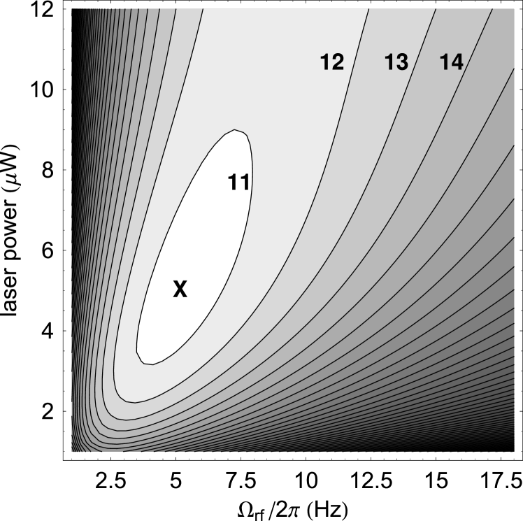
Figure 7: Plot of $\delta B_{\mathrm{NEM}}$ as a function of the amplitude $\Omega_{\mathrm{rf}}$ of the rotating field and of the laser power $P_{L}$. The contours represent the lines of constant $\mathrm{NEM}$, spaced by 1 $\mathrm{\mathrm{fT}}/\sqrt{\mathrm{Hz}}$, with selected numerical values indicated. The cross refers to the minimal $\mathrm{NEM}$ value, which, for the cell represented here has a value of 10.5 $\mathrm{\mathrm{fT}}/\sqrt{\mathrm{Hz}}$.

For each cell we have evaluated $\delta B_{\mathrm{NEM}}$ for a range of parameters $P_{L}$ and $\Omega_{\mathrm{rf}}$. Figure 7 shows a typical result in terms of a contour plot of $\delta B_{\mathrm{NEM}}$. For each cell we determine the optimal $\mathrm{NEM}$ value, $\delta B_{\mathrm{NEM}}^{\mathrm{min}}$, by a numerical minimization procedure. The minimum for the cell shown in Fig. 7 is indicated by a cross.

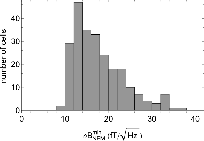
Figure 8: Histogram of the minimal $\mathrm{NEM}$ values, $\delta B_{\mathrm{NEM}}^{\mathrm{min}}$, of 241 cells, which represent 94% of the cells produced to date.

The distribution of minimal $\mathrm{NEM}$ values, $\delta B_{\mathrm{NEM}}^{\mathrm{min}}$, thus obtained is represented in form of a histogram in Fig. 8. Only cells with $\delta B_{\mathrm{NEM}}^{\mathrm{min}}<40\mathrm{\mathrm{fT}}/\sqrt{\mathrm{Hz}}$ are shown. This set represents 94% of all cells we have produced to date.

5 Discussion

The distribution of linewidths shown in Fig. 6 reveals a dependence of the form $\Gamma_{\kern-1.60997pt02}=\Gamma_{\kern-1.60997pt01}+\Delta\Gamma_{\kern-1.60997pt\mathrm{relax}}$, with a constant offset relaxation rate $\Delta\Gamma_{\kern-1.60997pt\mathrm{relax}}$, whose numerical value (fit parameter $a$ in Fig. 6) is $\Delta\Gamma_{\kern-1.60997pt\mathrm{relax}}/2\pi=1.35~{}\mathrm{Hz}$. Here we show that $\Gamma_{\kern-1.60997pt01}$ is ultimately limited by atoms escaping to the sidearm, and that $\Delta\Gamma_{\kern-1.60997pt\mathrm{relax}}$ is mainly determined by spin exchange collisions ($\Delta\Gamma_{\kern-1.60997pt\mathrm{ex}}$) with a minor contribution from magnetic field inhomogeneities ($\Delta\Gamma_{\kern-1.60997pt\Delta B}$).

5.1 Longitudinal relaxation

The intrinsic longitudinal relaxation rate $\Gamma_{\kern-1.60997pt01}$ is limited by processes which thermalize the magnetic sublevel populations, such as atoms escaping through the capillary to the sidearm where they eventually collide with the solid Cs droplet, atoms hitting an imperfectly coated surface spot of the spherical bulb, or atoms being absorbed by the coating Alexandrov:2002:LID ; Gozzini:2008:LIS . All of those processes can be parametrized in terms of an effective depolarizing surface area $\sigma_{\mathrm{dep}}\equiv\pi r_{\mathrm{dep}}^{2}$. We will refer to such processes in general as “reservoir losses”. The distribution of $\Gamma_{\kern-1.60997pt01}$ values in the top graph of Fig. 6 represents the statistical distribution of such imperfections, due to uncontrolled parameters in the cell production process. In a spherical cell of radius $R$ the rate of wall collisions is $\gamma_{\mathrm{wall}}=3\overline{v}/4R$, where $\overline{v}$ is the average thermal velocity. The intrinsic longitudinal relaxation rate can thus be expressed in terms of the effective depolarizing spot radius, $r_{\mathrm{dep}}$, via

$$\Gamma_{\kern-1.60997pt01}=\gamma_{\mathrm{wall}}\frac{\pi r_{\mathrm{dep}}^{2}}{4\pi R^{2}}=\frac{3\,\overline{v}\,r_{\mathrm{dep}}^{2}}{16\,R^{3}}\,.$$ (10)

The upper axis in the top graph of Fig. 6 shows the radius $r_{\mathrm{dep}}$ corresponding to the $\Gamma_{\kern-1.60997pt01}$ value on the lower axis. The best cell produced so far has a longitudinal relaxation rate $\Gamma_{\kern-1.60997pt01}/2\pi\approx 0.50(5)~{}\mathrm{Hz}$, which corresponds to $d_{\mathrm{dep}}=2r_{\mathrm{dep}}=1~{}\mathrm{mm}$. This value is compatible with the design diameter, $d_{\mathrm{cap}}=0.75(25)~{}\mathrm{mm}$, of the capillary, which shows that $\Gamma_{\kern-1.60997pt01}$ is ultimately limited by atoms escaping into the sidearm.

5.2 Transverse relaxation: field inhomogeneities

If the offset magnetic field $B_{0}$ varies over the cell volume it produces a distribution of resonance frequencies $\omega_{L}$, and hence a broadening of the magnetic resonance lines given by (2) and (3). The fitting analysis interprets this broadening as an increase of the transverse linewidth $\Gamma_{\kern-1.60997pt02}$ by an amount $\Delta\Gamma_{\Delta B}$. A main advantage of coated cells over buffer gas filled cells is that, because of multiple wall collisions, the atoms explore a large fraction of the cell volume during the spin coherence time, which effectively averages out field gradients. Standard line narrowing theory Watanabe:1977:MLN predicts that an inhomogeneous magnetic field gives a lowest order contribution

$$\Gamma_{\kern-1.60997pt\Delta B}=(\gamma_{F}\Delta B_{\mathrm{rms}})^{2}\tau_{c}$$ (11)

to the transverse relaxation rate, where $\Delta B_{\mathrm{rms}}$ is the rms value of the magnetic field averaged over the cell volume, and $\tau_{c}$ the correlation time of the field fluctuations seen by the cell, which can be approximated by the mean time between wall collisions. This expression is valid in the so-called good averaging regime Watanabe:1977:MLN , i.e., for $\gamma_{F}\Delta B_{\mathrm{rms}}\tau_{c}\ll 1$. From the geometry of the used coils we estimate $\Delta B_{\mathrm{rms}}$ to be on the order of 2 $\mathrm{nT}$, which yields $\Delta\nu_{\Delta B}=\Gamma_{\Delta B}/2\pi=30$ mHz. Even when allowing for a 5 times larger inhomogeneity (i.e., $\Delta B=10~{}\mathrm{nT}$) from uncompensated residual fields — recall that we actively compensate linear field gradients — one still has $\Delta\nu_{\Delta B}<0.1~{}\mathrm{Hz}$. We can thus ascertain that the contribution from field inhomogeneities to $\Gamma_{\kern-1.60997pt02}$ is negligible. We note that the good averaging conditions for $\Delta B=2~{}\mathrm{nT}$ and 10 $\mathrm{nT}$ read $\gamma_{F}\Delta B_{\mathrm{rms}}\tau_{c}=0.004$ and $0.02$, respectively.

5.3 Transverse relaxation: spin exchange

As derived by Ressler et al., Ressler:1969:MSE , the contribution from spin exchange collisions to the transverse relaxation rate is given by

$$\Delta\Gamma_{\kern-1.60997pt\mathrm{ex}}=\alpha\frac{2I}{2I+1}\,n_{\mathrm{Cs}}\sigma_{\mathrm{ex}}v_{r}\,,$$ (12)

where $I$ is the nuclear spin, $n_{\mathrm{Cs}}$ the Cs number density, $v_{r}$ the relative velocity of colliding atoms, and $\sigma_{\mathrm{ex}}=2.06\times 10^{-14}~{}\mathrm{cm}^{2}$ Ressler:1969:MSE the spin exchange cross section for Cs–Cs collisions. The parameter $\alpha$ describes the slowing down of the spin relaxation due to the hyperfine interaction. In small magnetic fields $\alpha\approx 0.63$ for the $M{=}-4\rightarrow M{=}-3$ transition (Fig. 3 of Ressler:1969:MSE ). At $T=20(1)\,{}^{\circ}$C the contribution of spin exchange collisions to $\Gamma_{\kern-1.60997pt02}$ evaluates to

$$\frac{\Delta\Gamma_{\kern-1.60997pt\mathrm{ex}}}{2\pi}=1.6(2)~{}\mathrm{Hz}\,,$$ (13)

where the error reflects the uncertainty in the number density. This value is compatible with the experimental value $\Gamma_{\kern-1.60997pt02}-\Gamma_{\kern-1.60997pt01}=(2\pi)1.35(3)~{}\mathrm{Hz}$. We are therefore confident that dephasing spin exchange collisions give the main contribution to the transverse relaxation rate, notwithstanding a certain scatter of the spin exchange cross sections in the literature.

5.4 Fundamental limits of magnetometric sensitivity

The ultimate sensitivity of the type of magnetometers described here is limited by two fundamental processes, viz., photon shot noise limit and spin projection noise. One can show (Appendix A) that the minimal $\mathrm{NEM}$ imposed by the shot noise of the detected photons is given by

$$\delta B_{\mathrm{NEM}}^{\mathrm{PSN}}=\frac{2\sqrt{2}\Gamma_{\kern-1.60997pt2}}{\gamma_{F}}\sqrt{\frac{\Gamma_{\kern-1.60997pt2}}{\Gamma_{\kern-1.60997pt1}}}\frac{1}{\kappa_{0}L}\frac{1}{A_{FF^{\prime}}\mathinner{\langle{F_{z}}\rangle}}\sqrt{\frac{h\nu}{{Q}_{\kern-1.39998ptE}P_{L}t}}\,,$$ (14)

where $P_{L}$ is the power detected after the cell, ${Q}_{\kern-1.39998ptE}$ the quantum efficiency of the photodiode for photons of energy $h\nu$, and $\kappa_{0}$ the resonant absorption coefficient of the driven hyperfine component for unpolarized atoms. For a time interval of $t=0.5$ s, the result corresponds to a measurement bandwidth of 1 $\mathrm{Hz}$. In (14) $\mathinner{\langle{F_{z}}\rangle}$ is the spin polarization

$$\mathinner{\langle{F_{z}}\rangle}=\sum_{M=-4}^{4}p_{4,M}^{\phantom{+}}M\,,$$ (15)

in the $F{=}4$ state, where the $p_{4,M}$ are the populations of the magnetic sublevels $\mathinner{|{F{=}4,M}\rangle}$. The analyzing power for the transition $F{\rightarrow}F^{\prime}$, $A_{FF^{\prime}}$, depends in general on the applied laser power and accounts for population effects such as hyperfine pumping. Its value has been determined by a numerical model based on rate equations pumping_inprep . It is a slowly varying function in the domain of laser powers considered here, with value $A_{43}=1.15(5)$.

For our apparatus, $\kappa_{0}L\approx 0.7$, ${Q}_{\kern-1.39998ptE}=0.7$, so the above can be rewritten as

$$\delta B_{\mathrm{NEM}}^{\mathrm{PSN}}(\mathrm{fT})=\frac{0.146}{A_{43}\mathinner{\langle{F_{z}}\rangle}\sqrt{P_{L}(\mu\mbox{W})}}\Gamma_{\kern-1.60997pt2}\sqrt{\frac{\Gamma_{\kern-1.60997pt2}}{\Gamma_{\kern-1.60997pt1}}}\,.$$ (16)

For our best cell, $A_{43}\mathinner{\langle{F_{z}}\rangle}=0.39(4)$, $\Gamma_{\kern-1.60997pt1}/2\pi=3.40~{}\mathrm{Hz}$, and $\Gamma_{\kern-1.60997pt2}/2\pi=4.75~{}\mathrm{Hz}$ at the optimum laser power of $3.6~{}\mu$W, which yields an expected sensitivity of $\delta B_{\mathrm{NEM}}^{\mathrm{PSN}}=7.0(7)~{}\mathrm{fT}$, to be compared with the measured minimal $\mathrm{NEM}$ of the cell of 9(1) $\mathrm{fT}$. For a more typical cell with $\Gamma_{\kern-1.60997pt2}/2\pi=10~{}\mathrm{Hz}$, $\Gamma_{\kern-1.60997pt1}/2\pi=8.65~{}\mathrm{Hz}$, and $A_{43}\mathinner{\langle{F_{z}}\rangle}=0.46(5)$ at the optimal power of $5~{}\mu$W, the expected minimal $\mathrm{NEM}$ is $\delta B_{\mathrm{NEM}}^{\mathrm{PSN}}=9.6(1.0)~{}\mathrm{fT}$, indicating that the shot noise limited $\mathrm{NEM}$ grows less than linearly in $\Gamma_{\kern-1.60997pt2}$.

Spin projection noise limits the magnetometric sensitivity to

$$\delta B_{\mathrm{NEM}}^{\mathrm{SPN}}=\frac{1}{\gamma_{F}}\sqrt{\frac{\Gamma_{\kern-1.60997pt2}}{N_{\mathrm{at}}t_{\mathrm{meas}}}}\,,$$ (17)

where $N_{\mathrm{at}}=\frac{9}{16}\rho_{\mathrm{at}}V_{\mathrm{cell}}$ is the number of atoms in the $F{=}4$ state that contribute to the signal, with $\rho_{\mathrm{at}}$ being the total Cs number density, and $V_{\mathrm{cell}}$ the cell volume. For a measurement time $t_{\mathrm{meas}}$ of 0.5 s, one finds at $T=20(1)\,{}^{\circ}$C, $\delta B_{\mathrm{NEM}}^{\mathrm{SPN}}=0.74(2)~{}\mathrm{fT}$ for $\Gamma_{\kern-1.60997pt2}/2\pi=4.75~{}\mathrm{Hz}$. In our magnetometers spin projection noise thus has a negligible contribution.

6 Summary and conclusion

We have manufactured and characterized a set of 253 paraffin-coated Cs vapor cells of identical geometry (15 mm radius spheres), 90% of which have an intrinsic transverse relaxation rate in the range of 2 to 6 $\mathrm{Hz}$. Under optimized conditions of laser and $\mathrm{rf}$ power those cells have intrinsic magnetometric sensitivities, $\delta B_{\mathrm{NEM}}^{\mathrm{min}}$, in the range of 9 to 30 $\mathrm{\mathrm{fT}}/\sqrt{\mathrm{Hz}}$ under the assumption of (light) shot-noise limited operation in a DROM-type magnetometer.

The magnetometric sensitivity is determined by the intrinsic transverse relaxation rate, which, for the best cell of our batch has a value of $2\pi\cdot 2~{}\mathrm{Hz}$, of which $\approx~{}0.5~{}\mathrm{Hz}$ are due to reservoir ($T_{1}$) relaxation, and $\approx~{}1.5~{}\mathrm{Hz}$ are due to spin exchange relaxation. Improving the relaxation properties by reducing reservoir relaxation is technologically demanding, and would only marginally improve the overall sensitivity. Spin exchange relaxation, on the other hand, cannot be suppressed in coated cells, although it was shown that spin exchange relaxation can be suppressed in high pressure buffer gas cells, yielding sub-$\mathrm{fT}$ magnetometric sensitivity Kominis:2003:SMA . We thus conclude that our cells are as good as coated cells of that diameter can be, disregarding a possible 25% reduction of $\Gamma_{\kern-1.60997pt02}/2\pi$ by a suppression of reservoir losses.

The expected photon shot noise limited $\mathrm{NEM}$ of our cells is very close to the measured $\mathrm{NEM}$. The most promising improvement in sensitivity is expected to come from maximizing $\mathinner{\langle{F_{z}}\rangle}$ via hyperfine repumping, which could win, at most, a factor of 2–3.

It is well known that in the spin exchange limited regime an increase of the atomic density by heating the cell does not increase the magnetometric sensitivity, since both $\Gamma_{\kern-1.60997pt2}$ and $\kappa_{0}$ in (14) grow proportionally to the density. The same holds for $\Gamma_{\kern-1.60997pt2}$ and $N_{\mathrm{atom}}$ in (17). However, when operating the magnetometer in a regime where spin exchange is not the limiting factor, one expects an improvement of the sensitivity by increasing the atomic number density.

We will use the cells in multi-sensor applications in fundamental and applied fields of research. Since an optimal magnetometric sensitivity is reached with a typical light power of approximately $5~{}\mu$W, a single diode laser can drive hundreds of individual sensors Hofer:2008:HSO . This scalability, together with the very good reproducibility of the coated cell quality reported here, will allow us to realize in the near future a three-dimensional array of 25 individual sensors for imaging the magnetic field of the beating human heart, a signal with a peak amplitude 100 $\mathrm{pT}$ Hofer:2008:HSO . With a reliable and inexpensive multichannel heart measurement system, magnetocardiograms can be measured in a few minutes, times which are of interest in the real world of clinical applications.

Appendix A Photon shot noise limit

Consider a light beam of power $P_{in}$ traversing a vapor of thickness $L$. The transmitted power detected by a photodiode with quantum efficiency ${Q}_{\kern-1.39998ptE}$ is given by

$$P_{det}(t)={Q}_{\kern-1.39998ptE}P_{in}e^{-\kappa(t)L}={Q}_{\kern-1.39998ptE}P_{L}\,.$$ (18)

The time dependent absorption coefficient $\kappa(t)$ considering the in-phase component of the magnetic-resonance induced modulation is

$$\kappa(t)=\kappa_{0}\left(1-A_{FF^{\prime}}\mathinner{\langle{F_{z}}\rangle}\frac{\Omega_{\mathrm{rf}}\delta}{\delta^{2}+\Gamma_{\kern-1.60997pt2}^{2}+\frac{\Gamma_{\kern-1.14998pt2}}{\Gamma_{\kern-1.14998pt1}}\Omega^{2}_{\mathrm{rf}}}\cos{\omega t}\right)\,,$$ (19)

where $\kappa_{0}$ is the resonant optical absorption coefficient for a sample of unpolarized atoms and the polarization $\mathinner{\langle{F_{z}}\rangle}$ is as defined by (15). The analyzing power for transition $F{\rightarrow}F^{\prime}$, $A_{FF^{\prime}}$, accounts for population effects such as hyperfine pumping: more details are given in the discussion in the main text following (15). Lock-in detection extracts from (18) the rms value

$$P^{LIA}_{det}=\frac{1}{\sqrt{2}}{Q}_{\kern-1.39998ptE}P_{in}e^{-\kappa_{0}L}\>\kappa_{0}LA_{FF^{\prime}}\mathinner{\langle{F_{z}}\rangle}\frac{\Omega_{\mathrm{rf}}\delta}{\delta^{2}+\Gamma_{\kern-1.60997pt2}^{2}+\frac{\Gamma_{\kern-1.14998pt2}}{\Gamma_{\kern-1.14998pt1}}\Omega^{2}_{\mathrm{rf}}}$$ (20)

of the in-phase component of the power modulation.

Light power $P$ can be converted to a photon count $N$ seen during time $t$ via $N=\frac{Pt}{h\nu}$, for $\nu$ the photon frequency. Hence $N^{LIA}_{det}$ represents the number of photons carrying magnetometric information, thus

$$\frac{dN^{LIA}_{det}}{dB}=\frac{dN^{LIA}_{det}}{dP^{LIA}_{det}}\frac{dP^{LIA}_{det}}{d\delta}\frac{d\delta}{dB}\,,$$ (21)

which evaluates to

$$\frac{dN^{LIA}_{det}}{dB}=\frac{1}{\sqrt{2}}\>\kappa_{0}Le^{-\kappa_{0}L}\>N_{in}{Q}_{\kern-1.39998ptE}A_{FF^{\prime}}\mathinner{\langle{F_{z}}\rangle}\frac{\gamma_{F}}{2\Gamma_{\kern-1.60997pt2}}\sqrt{\frac{\Gamma_{\kern-1.60997pt1}}{\Gamma_{\kern-1.60997pt2}}}\,,$$ (22)

assuming an $\mathrm{rf}$ amplitude ($\Omega_{\mathrm{rf}}=\sqrt{\Gamma_{\kern-1.60997pt2}\Gamma_{\kern-1.60997pt1}}$) which maximizes the result.

The photon shot noise limited magnetometric sensitivity is given by

$$\delta B_{\mathrm{NEM}}^{\mathrm{PSN}}=\sqrt{N^{DC}_{det}}\left(\frac{dN^{LIA}_{det}}{dB}\right)^{-1}\,,$$ (23)

where

$$N^{DC}_{det}=\left<{Q}_{\kern-1.39998ptE}N_{in}e^{-\kappa(t)L}\right>_{t}={Q}_{\kern-1.39998ptE}N_{in}e^{-\kappa_{0}L}\,.$$ (24)

Assembling the above components gives

$$\delta B_{\mathrm{NEM}}^{\mathrm{PSN}}=\frac{2\sqrt{2}\Gamma_{\kern-1.60997pt2}}{\gamma_{F}}\sqrt{\frac{\Gamma_{\kern-1.60997pt2}}{\Gamma_{\kern-1.60997pt1}}}\frac{1}{\kappa_{0}L}\frac{1}{A_{FF^{\prime}}\mathinner{\langle{F_{z}}\rangle}}\sqrt{\frac{h\nu}{{Q}_{\kern-1.39998ptE}P_{L}t}}\,,$$ (25)

which is the required result.

This work is financially supported by the Swiss National Science Foundation (#200020–111958, #200020-119820, #200020–113641) and by the Velux Foundation.

References

- (1) D. Budker, W. Gawlik, D. F. Kimball, S. M. Rochester, and V. V. Yashchuk, A. Weis, Reviews of Modern Physics 74, 1153 (2002).
- (2) H. G. Robinson, E. S. Ensberg, and H. G. Dehmelt, Bull. Am. Phys. Soc. 3 (1958).
- (3) G. Di Domenico, H. Saudan, G. Bison, P. Knowles, and A. Weis, Phys. Rev. A 76, 023407 (pages 10) (2007), URL http://link.aps.org/abstract/PRA/v76/e023407.
- (4) A. Weis and R. Wynands, Opt. Las. Engineer. 43, 387 (2005).
- (5) D. Budker and M. Romalis, Nature Physics 3, 227 (2007), URL http://dx.doi.org/10.1038/nphys566.
- (6) M. Klein, I. Novikova, D. F. Phillips, and R. L. Walsworth, Journal of Modern Optics 53, 2583 (2006).
- (7) T. Fernholz, H. Krauter, K. Jensen, J. F. Sherson, A. S. Sorensen, and E. S. Polzik, Physical Review Letters 101, 073601 (pages 4) (2008), URL http://link.aps.org/abstract/PRL/v101/e073601.
- (8) E. B. Alexandrov, M. V. Balabas, D. Budker, D. English, D. F. Kimball, C.-H. Li, and V. V. Yashchuk, Phys. Rev. A 66, 042903 (2002), URL http://prola.aps.org/abstract/PRA/v66/i4/e042903.
- (9) S. Gozzini, A. Lucchesini, L. Marmugi, and G. Postorino, The European Physical Journal D 47, 1 (2008), URL http://dx.doi.org/doi/10.1140/epjd/e2008-00015-5.
- (10) G. Bison, R. Wynands, and A. Weis, J. Opt. Soc. Am. B. 22, 77 (2005).
- (11) G. Bison, R. Wynands, and A. Weis, Appl. Phys. B 76, 325 (2003).
- (12) A. Weis, G. Bison, and A. S. Pazgalev, Phys. Rev. A 74, 033401 (pages 8) (2006), URL http://link.aps.org/abstract/PRA/v74/e033401.
- (13) A. Hofer, G. Bison, N. Castagna, P. Knowles, J. L. Schenker, and A. Weis, In Preparation (2008).
- (14) S. Groeger, G. Bison, J.-L. Schenker, R. Wynands, and A. Weis, Eur. Phys. J. D 38, 239 (2006).
- (15) G. Ban, K. Bodek, M. Daum, R. Henneck, S. Heule, M. Kasprzak, N. Khomytov, K. Kirch, A. Knecht, S. Kistryn, et al., Hyperfine Interactions 172, 41 (2006).
- (16) A. Andalkar and R. B. Warrington, Phys. Rev. A 65, 032708 (2002).
- (17) J. Vanier and C. Audoin, The Quantum Physics of Atomic Frequency Standards (Adam Hilger, Bristol and Philadelphia, 1989).
- (18) D. Budker, L. Hollberg, D. F. Kimball, J. Kitching, S. Pustelny, and V. V. Yashchuk, Phys. Rev. A 71, 012903 (pages 9) (2005), URL http://link.aps.org/abstract/PRA/v71/e012903.
- (19) E. B. Aleksandrov, M. V. Balabas, A. K. Vershovskii, A. E. Ivanov, N. N. Yakobson, V. L. Velichanskii, and N. V. Senkov, Opt. Spectrosc. 78, 325 (1995).
- (20) K. L. Corwin, Z. T. Lu, C. F. Hand, R. J. Epstain, and C. E. Wieman, Appl. Opt. 37, 3295 (1998).
- (21) G. Di Domenico, G. Bison, S. Groeger, P. Knowles, A. S. Pazgalev, M. Rebetez, H. Saudan, and A. Weis, Phys. Rev. A 74, 063415 (pages 8) (2006), URL http://link.aps.org/abstract/PRA/v74/e063415.
- (22) Wolfram Research, Inc., Mathematica, V5.2 (Wolfram Research, Inc., Champaign, Illinois, 2008).
- (23) S. F. Watanabe and H. G. Robinson, J. Phys. B–At. Mol. Opt. Phys. 10, 931 (1977).
- (24) N. W. Ressler, R. H. Sands, and T. E. Stark, Phys. Rev. 184, 102 (1969).
- (25) A. Weis et al. (2009), article in preparation.
- (26) I. K. Kominis, T. W. Kornack, J. C. Allred, and M. V. Romalis, Nature 422, 596 (2003).