A Chebychev propagator for inhomogeneous Schrödinger equations

Abstract

A propagation scheme for time-dependent inhomogeneous Schrödinger equations is presented. Such equations occur in time dependent optimal control theory and in reactive scattering. A formal solution based on a polynomial expansion of the inhomogeneous term is derived. It is subjected to an approximation in terms of Chebychev polynomials. Different variants for the inhomogeneous propagator are demonstrated and applied to two examples from optimal control theory. Convergence behavior and numerical efficiency are analyzed.

I Introduction

Inhomogeneous time-dependent Schrödinger equations,

$$i\hbar\frac{\partial}{\partial t}|\psi(t)\rangle=\boldsymbol{\mathsf{\hat{H}}}|\psi(t)\rangle+\boldsymbol{\mathsf{\hat{G}}}(t)|\varphi(t)\rangle\,,$$ (1)

arise in many formal solutions of quantum dynamics. In particular they have been employed in a time dependent treatment of reactive scattering NeuhauserCPC91 ; NeuhauserCPL92 and in optimal control theory using time-dependent targets KaiserJCP04 ; SerbanPRA05 ; KaiserCP06 ; WerschnikJPB07 or state-dependent constraints JoseMyPRA08 . In reactive scattering, the inhomogeneity results from the application of a projection operator NeuhauserJCP89 . This projector divides the Hilbert space of the reactive system into subspaces corresponding, respectively, to the reactants and to the products. A reduced description for only the products can be derived where the time-dependent Schrödinger equation contains an inhomogeneity, i.e. a source term that corresponds to the creation of the products NeuhauserCPL92 .

In optimal control theory (OCT), the inhomogeneity may be caused by a projection operator as well. For example, a partitioning of the Hilbert space is implemented by a projection operator in order to suppress population in a forbidden subspace JoseMyPRA08 . This leads to a formulation of OCT with a state-dependent constraint containing the projection operator. As a result the backward propagation of the OCT equations includes an inhomogeneity in the Schrödinger equation. This term corresponds to the suppression of probability amplitude in the forbidden subspace.

Generally, an inhomogeneous Schrödinger equation arises in OCT if a time-dependent target or a state-dependent constraint are utilized. In the common versions of OCT, see e.g. Refs. ZhuJCP98 ; JosePRA03 , the target is not explicitly time-dependent, it depends only on some final time $T$. The constraints enforce the Schrödinger equation and a minimization of the field energy. But for explicitly time-dependent targets KaiserJCP04 ; SerbanPRA05 ; KaiserCP06 ; WerschnikJPB07 or for a state-dependent constraint JoseMyPRA08 ; OhtsukiJCP04 the optimization functional contains a contribution of the form

$$\lambda\int_{0}^{T}g\left[\psi(t),\psi^{*}(t)\right]dt\,,$$

where the state $|\psi\rangle$ of the system enters at each time $t$.

For the solution of the standard homogeneous time-dependent Schrödinger equation, a number of numerical propagation schemes exist RonnieReview88 ; RonnieReview94 . The Chebychev propagator RonnieCheby84 offers the advantage of a numerically exact solution. The accuracy of the calculation is then determined by the machine precision of the computer and the error is uniformly distributed. The propagator is based on approximating the formal solution of the homogeneous time-dependent Schrödinger equation,

$$|\psi(t+dt)\rangle=e^{-\frac{i}{\hbar}\boldsymbol{\mathsf{\hat{H}}}dt}|\psi(t)\rangle\,,$$ (2)

by a series of Chebychev polynomials. Time-dependent inhomogeneous Schrödinger equations have been solved to date with split-propagator schemes SerbanPRA05 or via a full diagonalization of the Hamiltonian JoseMyPRA08 . While the latter method is numerically expensive and quickly becomes unfeasible with increasing system size, the first is of only limited accuracy.

Here, we derive a formal solution of the time-dependent inhomogeneous Schrödinger equation and we adapt it to the Chebychev propagation scheme. We apply this new propagator to the optimal control with a state-dependent constraint and with a time-dependent target. The paper is organized as follows: Section II presents the formal solution of Eq. (1). Propagation schemes for the formal solution are derived in Section III. The Chebychev propagation scheme is applied to OCT with a state-dependent constraint where the system is forced to remain in a subspace of the total Hilbert space in Section IV. In this case the operator $\boldsymbol{\mathsf{\hat{G}}}$ in Eq. (1) is independent of time, $\boldsymbol{\mathsf{\hat{G}}}(t)=\boldsymbol{\mathsf{\hat{G}}}$. In Section V, a second application, OCT with a time-dependent target, is studied keeping the full time-dependence, $\boldsymbol{\mathsf{\hat{G}}}(t)$. In both applications, the convergence of the new Chebychev propagator is analyzed in detail. Section VI concludes.

II Formal solution

The inhomogeneous Schrödinger equation, Eq. (1), is treated as an ordinary differential equation. It can be rewritten (setting $\hbar=1$)

$$i\frac{\partial}{\partial t}|\psi(t)\rangle=\boldsymbol{\mathsf{\hat{H}}}|\psi(t)\rangle+|\Phi(t)\rangle\,,$$ (3)

where $|\Phi(t)\rangle=\boldsymbol{\mathsf{\hat{G}}}(t)|\varphi(t)\rangle$. Eq. (3) is solved subject to the boundary conditions

$$|\psi(0)\rangle=|\psi_{0}\rangle\,,\quad\quad|\Phi(0)\rangle=|\Phi_{0}\rangle\,.$$ (4)

$|\Phi(t)\rangle$ is known globally in the propagation time interval, $[0,T]$, for example by a numerical representation on $N_{t}$ sampling points. $|\Phi(t)\rangle$ is assumed to be analytic, so that it can be interpolated to any arbitrary point within $[0,T]$. The representation of $|\Phi(t)\rangle$ on $N_{t}$ sampling points corresponds to an expansion in $N_{t}$ basis functions. Choosing equidistant sampling points yields a Fourier representation. A high-order (usually $N_{t}\gg 1$) polynomial expansion is obtained when the sampling points are chosen as roots of polynomials, implying non-equidistant time steps. The optimal representation treating correctly the boundaries is obtained by choosing Chebychev polynomials.

The basic idea consists in devising a short-time integration scheme for the interval $[0,t]$ (or, more generally $[t_{n},t_{n+1}]$ with $n,n+1\leq N_{t}$) by taking the following polynomial expansion of the inhomogeneous term,

$$|\Phi(t)\rangle\approx\sum_{j=0}^{m-1}P_{j}(\bar{\tau})|\bar{\Phi}_{j}\rangle\equiv\sum_{j=0}^{m-1}\frac{t^{j}}{j!}|\Phi^{(j)}\rangle\,.$$ (5)

Here, $P_{j}$ denotes the Chebychev polynomial of order $j$ with expansion coefficient $|\bar{\Phi}_{j}\rangle$, and $\bar{\tau}$ is a rescaled time, $\bar{\tau}=\frac{2\tau}{t}-1$, for $\tau\in[0,t]$. Note that the sum on the right-hand side of Eq. (5) is only of the form of a Taylor expansion for later manipulations but the approach itself is not based on a Taylor expansion. The Chebychev expansion coefficients $|\bar{\Phi}_{j}\rangle$ can be obtained e.g. by a cosine transformation (cf. Ref. RoiPRA00 and Section III.2 below). Once the coefficients $|\bar{\Phi}_{j}\rangle$ are known they are used to generate the coefficients $|\Phi^{(j)}\rangle$ in the second sum of Eq. (5), cf. Appendix A. This procedure has the advantage of employing a uniform approximation of $|\Phi^{(j)}\rangle$ in the interval $[0,t]$. However, if the function $|\Phi(t)\rangle$ is not known analytically, it needs to be interpolated at sampling points $\tau\in[0,t]$ in order to calculate the expansion coefficients $|\bar{\Phi}_{j}\rangle$. As a simpler alternative, the function $|\Phi^{(j)}\rangle$ is expanded in a Taylor series in the time interval $[0,t]$. Then the coefficients $|\Phi^{(j)}\rangle$ become the $j$th derivative of $|\Phi(t)\rangle$, at the beginning of the interval. At this point the properties of the global $N_{t}$ interpolation function of $|\Phi(t)\rangle$ are used to calculate $|\Phi^{(j)}\rangle$ as numerical derivatives at the beginning of each interval.

Based on Eq. (5), the solution of Eq. (3) can be written as

$$|\psi(t)\rangle_{(m)}=\sum_{j=0}^{m-1}\frac{t^{j}}{j!}|\lambda^{(j)}\rangle+\boldsymbol{\mathsf{\hat{F}}}_{m}|\lambda^{(m)}\rangle\,.$$ (6)

In Eq. (6), the subscript $m$ denotes the order of the solution. The $|\lambda^{(j)}\rangle$ are obtained iteratively,

$$|\lambda^{(0)}\rangle = |\psi_{0}\rangle\,,$$ (7)

$$|\lambda^{(j)}\rangle = -i\boldsymbol{\mathsf{\hat{H}}}|\lambda^{(j-1)}\rangle+|\Phi^{(j-1)}\rangle,$$

$$\quad\quad 1\leq j\leq m\,,$$

and $\boldsymbol{\mathsf{\hat{F}}}_{m}$ is a function of $\boldsymbol{\mathsf{\hat{H}}}$ given by

$$\boldsymbol{\mathsf{\hat{F}}}_{m}=f_{m}(\boldsymbol{\mathsf{\hat{H}}})=(-i\boldsymbol{\mathsf{\hat{H}}})^{-m}\left(e^{-i\boldsymbol{\mathsf{\hat{H}}}t}-\sum_{j=0}^{m-1}\frac{(-i\boldsymbol{\mathsf{\hat{H}}}t)^{j}}{j!}\right)\,.$$ (8)

Equations (6)-(8) represent the formal solution to the inhomogeneous Schrödinger equation.

In order to verify that Eq. (6) is indeed a solution to Eq. (3), let’s take the derivative of Eq. (6),

$$\frac{\partial}{\partial t}|\psi(t)\rangle_{(m)} = \sum_{j=0}^{m-1}j\frac{t^{j-1}}{j!}|\lambda^{(j)}\rangle+(-i\boldsymbol{\mathsf{\hat{H}}})^{-m}\left((-i\boldsymbol{\mathsf{\hat{H}}})e^{-i\boldsymbol{\mathsf{\hat{H}}}t}-\sum_{j=1}^{m-1}j(-i\boldsymbol{\mathsf{\hat{H}}})\frac{(-i\boldsymbol{\mathsf{\hat{H}}}t)^{j-1}}{j(j-1)!}\right)|\lambda^{(m)}\rangle$$

$$= \sum_{j=0}^{m-2}\frac{t^{j}}{j!}|\lambda^{(j+1)}\rangle+(-i\boldsymbol{\mathsf{\hat{H}}})(-i\boldsymbol{\mathsf{\hat{H}}})^{-m}\left(e^{-i\boldsymbol{\mathsf{\hat{H}}}t}-\sum_{j=0}^{m-2}\frac{(-i\boldsymbol{\mathsf{\hat{H}}}t)^{j}}{j!}\right)|\lambda^{(m)}\rangle\,.$$

Inserting Eq. (7) in the first term and resumming with an upper limit $m-1$, one obtains

$$\frac{\partial}{\partial t}|\psi(t)\rangle_{(m)} = \sum_{j=0}^{m-1}\frac{t^{j}}{j!}\left(-i\boldsymbol{\mathsf{\hat{H}}}|\lambda^{(j)}\rangle+|\Phi^{(j)}\rangle\right)-\frac{t^{m-1}}{(m-1)!}\left(-i\boldsymbol{\mathsf{\hat{H}}}|\lambda^{(m-1)}\rangle+|\Phi^{(m-1)}\rangle\right)$$

$$\quad\quad\quad-i\boldsymbol{\mathsf{\hat{H}}}(-i\boldsymbol{\mathsf{\hat{H}}})^{-m}\left(e^{-i\boldsymbol{\mathsf{\hat{H}}}t}-\sum_{j=0}^{m-1}\frac{(-i\boldsymbol{\mathsf{\hat{H}}}t)^{j}}{j!}+\frac{(-i\boldsymbol{\mathsf{\hat{H}}}t)^{m-1}}{(m-1)!}\right)|\lambda^{(m)}\rangle\,.$$

Recognizing $\boldsymbol{\mathsf{\hat{F}}}_{m}$, cf. Eq. (8), as part of the last term and inserting $|\lambda^{(j)}\rangle$, cf. Eq. (7), in the second term, which then cancels with the second summand of the last term, this can be rewritten

$$\frac{\partial}{\partial t}|\psi(t)\rangle_{(m)} = -i\boldsymbol{\mathsf{\hat{H}}}\left(\sum_{j=0}^{m-1}\frac{t^{j}}{j!}|\lambda^{(j)}\rangle+\boldsymbol{\mathsf{\hat{F}}}_{m}|\lambda^{(m)}\rangle\right)$$

$$+\sum_{j=0}^{m-1}\frac{t^{j}}{j!}|\Phi^{(j)}\rangle\,.$$

The expression in parenthesis corresponds to $|\psi(t)\rangle$, cf. Eq. (6). Finally, replacing the second term by $|\Phi(t)\rangle$, cf. Eq. (5), the inhomogeneous Schrödinger equation, Eq. (3), is obtained. Therefore Eq. (6) presents indeed a solution to Eq. (3).

III Propagation schemes

The formal solution, Eq. (6), is subjected to a spectral approximation,

$$|\psi(t)\rangle_{(m)N}=\sum_{j=0}^{m-1}\frac{t^{j}}{j!}|\lambda^{(j)}\rangle+P_{N(m)}(\boldsymbol{\mathsf{\hat{H}}})|\lambda^{(m)}\rangle\,,$$ (9)

where $P_{N}$ is a polynomial of order $N$ approximating $\boldsymbol{\mathsf{\hat{F}}}_{m}=f_{m}(\boldsymbol{\mathsf{\hat{H}}})$. For example, to first order, $m=1$, the formal solution is given by

$$|\psi(t)\rangle_{(1)}=e^{-i\boldsymbol{\mathsf{\hat{H}}}t}|\psi_{0}\rangle+(-i\boldsymbol{\mathsf{\hat{H}}})^{-1}(e^{-i\boldsymbol{\mathsf{\hat{H}}}t}-\leavevmode\hbox{\small 1\kern-3.3pt\normalsize 1})|\Phi_{0}\rangle\,.$$ (10)

In principle one might seek a spectral approximation for each of the terms. However, it is numerically more efficient to rewrite the first order solution,

$$|\psi(t)\rangle_{(1)}=|\psi_{0}\rangle+f_{1}(\boldsymbol{\mathsf{\hat{H}}})\left(-i\boldsymbol{\mathsf{\hat{H}}}|\psi_{0}\rangle+|\Phi_{0}\rangle\right)\,,$$ (11)

with $f_{1}(\boldsymbol{\mathsf{\hat{H}}})=(-i\boldsymbol{\mathsf{\hat{H}}})^{-1}(e^{-i\boldsymbol{\mathsf{\hat{H}}}t}-\leavevmode\hbox{\small 1\kern-3.3pt\normalsize 1})$, such that only a single Chebychev expansion plus one extra application of the Hamiltonian are required. Similarly, to second and third order the formal solutions can be written

$$|\psi(t)\rangle_{(2)} = |\psi_{0}\rangle+t|\lambda^{(1)}\rangle+f_{2}(\boldsymbol{\mathsf{\hat{H}}})|\lambda^{(2)}\rangle\,,$$ (12)

$$|\psi(t)\rangle_{(3)} = |\psi_{0}\rangle+t|\lambda^{(1)}\rangle+\frac{t^{2}}{2}|\lambda^{(2)}\rangle$$ (13)

$$+f_{3}(\boldsymbol{\mathsf{\hat{H}}})|\lambda^{(3)}\rangle$$

with $f_{2}(\boldsymbol{\mathsf{\hat{H}}})$ and $f_{3}(\boldsymbol{\mathsf{\hat{H}}})$ given by Eq. (8) and $|\lambda^{(j)}\rangle$ by Eq. (7). The strategy is then to seek a polynomial approximation for the functions $f_{j}(\boldsymbol{\mathsf{\hat{H}}})$. For $f_{0}(\boldsymbol{\mathsf{\hat{H}}})=e^{-i\boldsymbol{\mathsf{\hat{H}}}t}$, this corresponds to the standard Chebychev propagator for the homogeneous Schrödinger equation RonnieCheby84 . It will be briefly reviewed for clarity, followed by a discussion of the polynomial approximation of the new functions.

III.1 General idea of the Chebychev propagator

The Chebychev propagator is based on treating the formal solution as a function of an operator which is applied to some state vector,

$$|\phi\rangle=f(\boldsymbol{\mathsf{\hat{H}}})|\psi\rangle\,,$$

and to approximate this function by an expansion in Chebychev polynomials $P_{n}$,

$$f(\boldsymbol{\mathsf{\hat{H}}})|\psi\rangle=\sum_{n}a_{n}P_{n}(\boldsymbol{\mathsf{\hat{H}}})|\psi\rangle\,.$$

Since the Chebychev polynomials are defined within the range $[-1,1]$, the Hamiltonian has to be renormalized,

$$\boldsymbol{\mathsf{\hat{H}}}_{norm}=2\frac{\boldsymbol{\mathsf{\hat{H}}}-E_{min}\leavevmode\hbox{\small 1\kern-3.3pt\normalsize 1}}{\Delta E}-\leavevmode\hbox{\small 1\kern-3.3pt\normalsize 1}\,,$$

where $E_{min}$ denotes the smallest eigenvalue of $\boldsymbol{\mathsf{\hat{H}}}$ and $\Delta E=E_{max}-E_{min}$ the spectral range of $\boldsymbol{\mathsf{\hat{H}}}$. The wavefunction propagated from time zero to $t$ is then obtained by

$$|\psi(t)\rangle\approxeq e^{-i(\frac{1}{2}\Delta E+E_{min})t}\sum_{n=0}^{N}a_{n}P_{n}(-i\boldsymbol{\mathsf{\hat{H}}}_{norm})|\psi_{0}\rangle\,,$$

where the phase factor in front of the sum is due to the renormalization.

The algorithm to estimate $|\phi\rangle=f(\boldsymbol{\mathsf{\hat{H}}})|\psi\rangle$ proceeds as follows:

1. Calculate the expansion coefficients $a_{n}$,

   $$a_{n}=\frac{2-\delta_{n}}{\pi}\int_{-1}^{1}\frac{f(x)P_{n}(x)}{\sqrt{1-x^{2}}}dx\,.$$ (14)

   For the function $f(x)=f_{0}(x)=e^{-ixt}$, the integrals can be solved analytically resulting in the Bessel functions RonnieCheby84 .

2. Calculate $P_{n}(-i\boldsymbol{\mathsf{\hat{H}}}_{norm})|\psi_{0}\rangle$ using the recursion relation of the Chebychev polynomials,

   $$|\phi_{0}\rangle = |\psi_{0}\rangle\,,$$

   $$|\phi_{1}\rangle = -i\boldsymbol{\mathsf{\hat{H}}}_{norm}|\psi_{0}\rangle\,,$$ (15)

   $$|\phi_{n}\rangle = -2i\boldsymbol{\mathsf{\hat{H}}}_{norm}|\phi_{n-1}\rangle+|\phi_{n-2}\rangle\,.$$

3. Accumulate the result, taking into account the phase factor due to renormalization,

   $$|\psi(t)\rangle=e^{-i(\frac{1}{2}\Delta E+E_{min})t}\sum_{n=0}^{N}a_{n}|\phi_{n}\rangle\,.$$

Task 1 has to be performed only once, while 2 and 3 are repeated for each propagation step. The number $N$ of Chebychev polynomials is chosen such that the coefficient $a_{N+1}$ becomes smaller than some specified error $\varepsilon$. Since the coefficients can be determined analytically, $\varepsilon$ may correspond to the machine precision of the computer.

III.2 Chebychev propagator for inhomogeneous equations

According to Eqs. (10-13) a single Chebychev expansion plus a few applications of the Hamiltonian are required to solve the inhomogeneous Schrödinger equation. In particular, the application of a function $f_{m}(\boldsymbol{\mathsf{\hat{H}}})$ to a state vector $|\lambda^{(m)}\rangle$ has to be considered,

$$|\phi\rangle=f_{m}(\boldsymbol{\mathsf{\hat{H}}})|\lambda^{(m)}\rangle\,,$$ (16)

where $|\lambda^{(m)}\rangle$ is obtained recursively by Eq. (7). The Chebychev propagation scheme now consists in calculating $|\lambda^{(m)}\rangle$ and performing tasks 1–3 for $f_{m}(\boldsymbol{\mathsf{\hat{H}}})|\lambda^{(m)}\rangle$ instead of $f_{0}(\boldsymbol{\mathsf{\hat{H}}})|\lambda^{(m)}\rangle$. There are two differences with respect to the standard Chebychev propagator, i.e. between the approximation of $f_{0}(\boldsymbol{\mathsf{\hat{H}}})$ and the approximation of $f_{m>0}(\boldsymbol{\mathsf{\hat{H}}})$.

(i) For $m>0$, the integrals required to calculate the expansion coefficients $a_{n}$, Eq. (14), cannot be solved analytically anymore. They can, however, be obtained numerically with sufficient efficiency and accuracy RoiPRA00 . The approach of Ref. RoiPRA00 is repeated here for completeness: Applying a Gaussian quadrature to the Chebychev polynomials, the integral in Eq. (14) is rewritten,

$$a_{n}=\frac{2-\delta_{n0}}{N}\sum_{k=0}^{N-1}f_{m}(x_{k})P_{n}(x_{k})\,,$$ (17)

where the sampling points $x_{k}$ correspond to the $N$ roots of the Polynomial $P_{N}$,

$$x_{k}=\cos\left(\frac{\pi(k+\frac{1}{2})}{N}\right)\,,k=0,\,\ldots\,N-1\,.$$ (18)

Since the Chebychev polynomials can be expressed in terms of cosines, $P_{n}(x)=\cos(n\theta)$ with $\theta=\arccos(x)$, Eq. (17) corresponds to a cosine transformation,

$$a_{n}=\frac{2-\delta_{n0}}{N}\sum_{k=0}^{N-1}f_{m}(\theta_{k})\cos(n\theta_{k})\,.$$ (19)

The expansion coefficients are thus most easily evaluated by Fast Cosine Transformations.

Special care is, however, required for small values of the argument of $f_{m}(\boldsymbol{\mathsf{\hat{H}}})$ since $f_{m}(\boldsymbol{\mathsf{\hat{H}}})$ involves division by the $m$th power of $\boldsymbol{\mathsf{\hat{H}}}$. It is recommended to employ the definition of $f_{m}(\boldsymbol{\mathsf{\hat{H}}})$, Eq. (8), only if the argument is larger than some small value $\epsilon$ and to use a Taylor expansion of $f_{m}(\boldsymbol{\mathsf{\hat{H}}})$,

$$f_{m>0}(\boldsymbol{\mathsf{\hat{H}}})=t^{m}\sum_{j=0}^{\infty}\frac{(-i\boldsymbol{\mathsf{\hat{H}}}t)^{j}}{(j+m)!}$$ (20)

for arguments smaller than $\epsilon$.

(ii) As explained in Section II, a Taylor expansion of $|\Phi(t)\rangle$ for each integration interval $[0,t]$ is most easily used if the inhomogeneous term is represented numerically at sampling points. Recursive calculation of $|\lambda^{(m)}\rangle$ then requires numerical evaluation of the time derivatives of the ’inhomogeneous state vector’, $|\Phi(t)\rangle$. Second order $m=2$ requires the first derivative which can be obtained with sufficient accuracy by Fast Fourier Transformation (FFT) and multiplication in frequency domain. However, an error is introduced due to finite values of $|\Phi(t)\rangle$ at the boundaries of the grid, i.e. $t=0$ and $t=T$. This error is increased and propagated throughout the time interval in the calculation of higher order derivatives by FFT and multiplication in frequency domain.

Higher order schemes require therefore a different method for the evaluation of the derivatives. A suitable choice represents $|\Phi(t)\rangle$ by an expansion into Chebychev polynomials. The derivatives are then calculated recursively based on the analytical properties of the Chebychev polynomials Dunn96 . Note that this implies a non-equidistant time grid since the roots of the Chebychev polynomials need to be taken as sampling points,

$$t^{\prime}_{n}=\cos\left(\frac{n\pi}{N_{t}-1}\right)\,,\,t_{n} = \frac{T}{2}\left(1+\cos\left(\frac{n\pi}{N_{t}-1}\right)\right)\,,$$

$$n = 0,\ldots,N_{t}-1\,,$$

where the time interval $t\in[0,T]$ is scaled to $t^{\prime}\in[-1,1]$ and $N_{t}$ denotes the number of sampling points. A non-equidistant time grid requires calculation and storage of the Chebychev expansion coefficients of the propagator for each $\Delta t_{n}$. This additional effort is well paid off since a higher order scheme allows for larger time steps, i.e. smaller $N_{t}$.

III.3 Summary of the Algorithm

The algorithm to solve the inhomogeneous time-dependent Schrödinger equation is summarized in order to outline the flow chart of the numerical implementation:

1. Set the time grid $\{t_{n}\}$ and determine the inhomogeneous term $|\Phi(t_{n})\rangle$.

2. Calculate the Chebychev expansion coefficients of $\boldsymbol{\mathsf{\hat{F}}}_{m}=f_{m}(\boldsymbol{\mathsf{\hat{H}}})$, cf. Eq. (8). This needs to be done for each time step size that occurs in a time grid with non-equidistant steps or only once if an equidistant time grid is employed.

3. Determine all $|\Phi^{(j)}\rangle$ required in Eqs. (6) and (7). This is done differently whether the uniform approximation or the Taylor expansion over the short-time interval $[0,t]$ is employed.

   Uniform approximation (Chebychev expansion):

   1. Determine Chebychev sampling points $\{\tau_{k}\}$ within each short-time interval $[0,t]$ (or, generally, $[t_{n},t_{n+1}]$), cf. Eq. (18), and determine the value of $|\Phi(\tau_{k})\rangle$ analytically or by numerical interpolation.

   2. Calculate the Chebychev expansion coefficients $|\bar{\Phi}_{j}\rangle$ of $|\Phi(\tau_{k})\rangle$ by cosine transformation analogously to Eq. (19) with $f_{m}$ replaced by $|\Phi\rangle$.

   3. Derive $|\Phi^{(j)}\rangle$ for all $\{t_{n}\}$ from $|\bar{\Phi}_{j}\rangle$ using the transformation between a Chebychev and a Taylor expansion given in Appendix A, i.e. employing the recursive relations given in Eqs. (44) and (A).

   Taylor expansion:
   Calculate $|\Phi^{(j)}\rangle$ as time derivatives of $|\Phi(t_{n})\rangle$ either by FFT for equidistant time grid or by numerical differentiation based on the analytical properties of Chebychev polynomials Dunn96 for non equidistant time steps.

4. Perform the time propagation, i.e. for each time step from 0 to $t$ (or, generally, $t_{n}$ to $t_{n+1}$),

   1. determine $|\lambda^{(j)}\rangle$ according to Eq. (7),

   2. obtain $\boldsymbol{\mathsf{\hat{F}}}_{m}|\lambda^{(j)}\rangle$ by Chebychev recursion, cf. Eq. (2),

   3. evaluate $|\Psi(t)\rangle$ (or, generally, $|\Psi(t_{n+1})\rangle$) according to Eq. (6).

In order to avoid storage of the Chebychev expansion coefficients, step 2 in the case of a non-equidistant time grid and step 3 in the case of the uniform approximation may also be performed during the time propagation in step 4.

The algorithm to solve the inhomogeneous time-dependent Schrödinger equation requires adjustment of two parameters – the order of the algorithm, $m$, and the propagation time step, i.e. the size of the short-time interval. The latter can also be specified in terms of the overall number of time steps, $N_{t}$, which is particularly useful for non-equidistant time steps. The two parameters are linked to each other: Employing a higher order $m$ allows for taking larger time steps, or, equivalently, reducing $N_{t}$. A detailed discussion how the two parameters should be chosen is presented for the applications in Sections IV and V below.

III.4 Approximation of the formal solution by a Taylor expansion

A simplified version of the algorithm is devised by approximating the formal solution explicitly by a Taylor expansion. This yields a standard Chebychev propagator plus additional terms involving derivatives of $|\Phi(t)\rangle$. An existing Chebychev propagation code then needs little modification to be adapted to an inhomogeneous Schrödinger equation. The accuracy of the simplified algorithm is, however, limited by the Taylor expansion.

As shown in Appendix B, the formal solution, Eq. (6), can be written as

$$|\psi(t)\rangle_{(m)}=e^{-i\boldsymbol{\mathsf{\hat{H}}}t}|\psi_{0}\rangle+\sum_{j=0}^{m-1}\boldsymbol{\mathsf{\hat{F}}}_{j+1}|\Phi^{(j)}\rangle\,,$$ (21)

with

$$\boldsymbol{\mathsf{\hat{F}}}_{j+1}=(-i\boldsymbol{\mathsf{\hat{H}}})^{-(j+1)}\left(e^{-i\boldsymbol{\mathsf{\hat{H}}}t}-\sum_{k=0}^{j}\frac{(-i\boldsymbol{\mathsf{\hat{H}}}t)^{k}}{k!}\right).$$

Taking the Taylor expansion of the exponential in $\boldsymbol{\mathsf{\hat{F}}}_{j+1}$ up to order $j+1$,

$$e^{-i\boldsymbol{\mathsf{\hat{H}}}t}=\sum_{k=0}^{j+1}\frac{(-i\boldsymbol{\mathsf{\hat{H}}}t)^{k}}{k!}=\sum_{k=0}^{j}\frac{(-i\boldsymbol{\mathsf{\hat{H}}}t)^{k}}{k!}+\frac{(-i\boldsymbol{\mathsf{\hat{H}}}t)^{j+1}}{(j+1)!}\,,$$

one obtains an approximation of Eq. (21),

$$|\psi(t)\rangle_{(m)}\approx e^{-i\boldsymbol{\mathsf{\hat{H}}}t}|\psi_{0}\rangle+\sum_{j=0}^{m-1}\frac{t^{j+1}}{(j+1)!}|\Phi^{(j)}\rangle\,.$$ (22)

To all orders, only the standard Chebychev propagation scheme plus calculation and storage of the derivatives of the inhomogeneous term, $|\Phi^{(j)}\rangle$, are required. For example, the approximate solution to second order reads

$$|\psi(t)\rangle_{(2)}\approx f_{0}(\boldsymbol{\mathsf{\hat{H}}})|\psi_{0}\rangle+t|\Phi^{(0)}\rangle+\frac{t^{2}}{2}|\Phi^{(1)}\rangle\,.$$ (23)

Unlike the propagator described in Sections III.2 and III.3, this scheme is explicitly based on a Taylor expansion. It is therefore expected to be valid only for small time steps. In that case, a low order scheme (e.g. $m=2$) is sufficient. The necessary derivatives can then be calculated by FFT and multiplication in frequency domain. The validity of this approximation is discussed in detail in Section IV.2.

IV Application I: Control with a state-dependent constraint

In our first example, the operator occuring in the inhomogeneous term is not time-dependent, $\boldsymbol{\mathsf{\hat{G}}}(t)=\boldsymbol{\mathsf{\hat{G}}}$.

IV.1 Model

A simplified model of the vibrations in a Rb₂ molecule is considered taking into account three electronic states JoseMyPRA08 . The corresponding Hamiltonian reads

$$\boldsymbol{\mathsf{\hat{H}}} \,=\, \sum_{i=1}^{3}\boldsymbol{\mathsf{\hat{H}}}_{i}\otimes|e_{i}\rangle\langle e_{i}|+\boldsymbol{\mathsf{\hat{\mu}}}\,\epsilon(t)\cdot\,\bigg{(}|e_{1}\rangle\langle e_{2}|+$$

$$|e_{2}\rangle\langle e_{1}|+|e_{2}\rangle\langle e_{3}|+|e_{3}\rangle\langle e_{2}|\bigg{)}\,,$$

where $\boldsymbol{\mathsf{\hat{H}}}_{i}$ denotes the vibrational Hamiltonians, $\boldsymbol{\mathsf{\hat{H}}}_{i}=\boldsymbol{\mathsf{\hat{T}}}+V_{i}(\boldsymbol{\mathsf{\hat{R}}})$, $\boldsymbol{\mathsf{\hat{\mu}}}$ the transition dipole operator, assumed to be independent of $\boldsymbol{\mathsf{\hat{R}}}$, and $\epsilon(t)$ the electric field. The electronic states are associated to $X^{1}\Sigma_{g}^{+}(5s+5s)$, ${}^{1}\Sigma_{u}^{+}(5s+5p)$ and ${}^{1}\Pi_{g}(5s+4d)$, with the potentials found in Ref. ParkJMS01 .

OCT is tested for the objective of population transfer from the vibrational ground state of the electronic ground surface to a particular vibrationally excited state via Raman transitions between the ground and the second electronic surface. For strong laser fields $\epsilon(t)$, such as those found by OCT algorithms, population at intermediate times will be excited not only to the second but also to the third electronic surface. This is particularly the case for the electronic states of our example, where transition frequencies and Franck-Condon factors for transitions between $|e_{1}\rangle$ and $|e_{2}\rangle$ are very similar to those for transitions between $|e_{2}\rangle$ and $|e_{3}\rangle$. Assuming that the third electronic state corresponds to a loss channel, e.g. an intermediate state in resonantly enhanced multi-photon ionization or an autoionizing state, population transfer into this state should be avoided at all times. This can be communicated to the OCT algorithm by formulating a state-dependent constraint which maximizes the projection onto the allowed subspace JoseMyPRA08 , i.e. onto electronic states 1 and 2. The complete functional for optimization is then given by JoseMyPRA08

$$J[\varphi,\varphi^{*},\epsilon]=J_{0}[\varphi_{T},\varphi_{T}^{*}]\,+\,J_{a}[\epsilon]\,+\,J_{b}[\varphi,\varphi^{*}]$$ (25)

with

$$J_{0}[\varphi_{T},\varphi_{T}^{*}] = \lambda_{0}\,\langle\varphi(T)|\boldsymbol{\mathsf{\hat{D}}}|\varphi(T)\rangle\,,$$ (26)

$$J_{a}[\epsilon] = \int_{0}^{T}\lambda_{a}(t)\,[\epsilon(t)-\epsilon_{r}(t)]^{2}\,dt\,,$$ (27)

$$J_{b}[\varphi,\varphi^{\dagger}] = \int_{0}^{T}\lambda_{b}\langle\varphi(t)|\boldsymbol{\mathsf{\hat{P}}}_{\mathrm{allow}}|\varphi(t)\rangle\,dt\,.$$ (28)

The operator $\boldsymbol{\mathsf{\hat{D}}}$ in $J_{0}$ is given by the projector onto the target level in the electronic ground state. The state-dependent constraint contains the projector onto the allowed subspace, $\boldsymbol{\mathsf{\hat{P}}}_{\mathrm{allow}}$. In Ref. JoseMyPRA08 , propagation via full diagonalization of the Hamiltonian was employed and only 11 vibrational levels in each electronic state were considered. Representing the vibrational Hamiltonians on a Fourier grid RonnieReview88 and utilizing the inhomogeneous Chebychev propagator, the full potentials can be taken into account ($N_{\mathrm{grid}}=128$).

IV.2 Test of the propagator

In order to test the new Chebychev propagator, our numerical results are compared to those obtained by the symmetrical method for the Hamiltonian comprising of 11 levels in each electronic state JoseMyPRA08 . The details of the symmetrical method are reviewed in Appendix C. The inhomogeneous Schrödinger equation reads JoseMyPRA08

$$\frac{d}{dt}|\psi(t)\rangle\,=\,-\frac{i}{\hbar}\,\boldsymbol{\mathsf{\hat{H}}}[\epsilon(t)]\,|\psi(t)\rangle\,+\,\lambda_{b}\boldsymbol{\mathsf{\hat{P}}}_{\mathrm{allow}}|\varphi(t)\rangle\,,$$ (29)

with the “initial” condition

$$|\psi(t=T)\rangle\,=\,-\lambda_{0}\,\boldsymbol{\mathsf{\hat{D}}}\,|\varphi(T)\rangle\,.$$ (30)

In OCT, $|\psi(t)\rangle$ is the backward propagated wavefunction which is coupled to $|\varphi(t)\rangle$ obtained by forward propagation,

$$\frac{d}{dt}|\varphi(t)\rangle\,=\,-\frac{i}{\hbar}\boldsymbol{\mathsf{\hat{H}}}[\epsilon(t)]|\varphi(t)\rangle$$ (31)

with $|\varphi(t=0)\rangle\,=\,|\varphi_{0}\rangle$. The convergence with respect to the time step $\Delta t$ and the order $m$ of the Chebychev method will be discussed in Section  IV.3.

We start by propagating the initial state, $v=0$ of the electronic ground state, forward with a Gaussian pulse given by Eq. (33) of Ref. JoseMyPRA08 . The inhomogeneous Schrödinger equation is then propagated backward with the same field. All parameters are taken to be equal to those of Ref. JoseMyPRA08 .

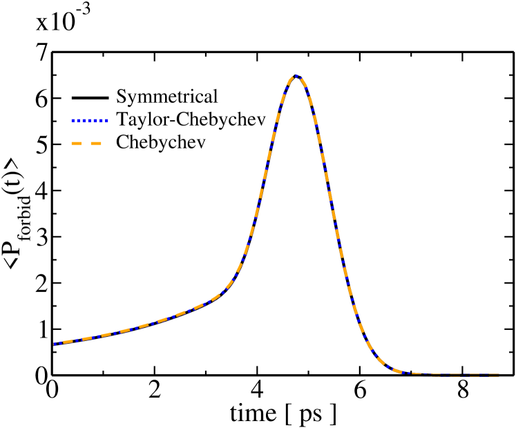
Figure 1: (color online) Normalized expectation value of the projector onto the forbidden subspace for a single backward propagation with a Gaussian pulse. Comparison between the symmetrical scheme of Ref. JoseMyPRA08 with $\Delta t=1\,$a.u. (black solid line), the Chebychev propagator in first order with $\Delta t=1\,$a.u. (orange dashed line) and the Chebychev propagator in first order based on the Taylor approximation, Eq.(22), with $\Delta t=0.1\,$a.u. (blue dotted line).

Figure 1 shows the expectation value of the projector onto the forbidden subspace, $\langle\boldsymbol{\mathsf{\hat{P}}}_{forbid}\rangle(t)$, for normalized $|\psi(t)\rangle$. Results for the symmetrical method and the first order Chebychev propagators based on Eq. (6) and on Eq. (22) (Taylor) are compared. A good agreement between the Chebychev propagators and the symmetrical scheme is found. The time step needed to obtain converged results with the approximate solution is, however, smaller by a factor of ten. This is not surprising since the approximate solution is based on a Taylor expansion which requires a very small $\Delta t$.

Our main motivation for the development of the modified Chebychev propagator lies in its application in OCT with a state-dependent constraint or a time-dependent target. Therefore the new propagator is also tested in an iterative solution of the control equations. The control problem is that of Ref. JoseMyPRA08 . However, in the present work the full vibrational Hamiltonians are employed.

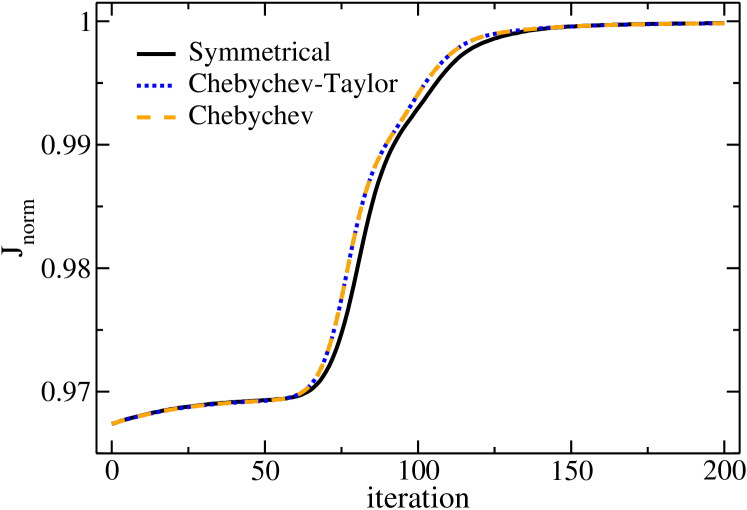
Figure 2: (color online) $J_{\mathrm{norm}}$ as a function of the number of iterations. Solution obtained by the symmetrical scheme of Ref. JoseMyPRA08 with a time step $\Delta t=1\,$a.u. (black solid line), the Chebychev propagator for first order with a time step $\Delta t=1\,$a.u. (orange dashed line) and the second order approximate solution of Eq.(22) with a time step $\Delta t=0.1\,$a.u. (blue dotted line).

Convergence of the OCT algorithm is measured by the normalized functional, $J_{\mathrm{norm}}=J/(\lambda_{0}+\lambda_{b}T)$, approaching one as the control equations are iteratively solved, cf. Fig. 2. The symmetrical scheme ($\Delta t=1\,$a.u., black solid line) is compared to the Chebychev propagator in first order (orange dashed line) and to the Chebychev propagator based on the Taylor approximation, Eq. (22), (blue dotted line) in second order. An overall good agreement is found. The difference between the results at intermediate iterations is attributed to the different models, the full vibrational Hamiltonian in the case of the Chebychev propagators and the Hamiltonian consisting of 33 levels in the case of the symmetrical method.

Application of the Chebychev propagator based on the Taylor approximation, Eq. (22), in first order failed: The inhomogeneous Schrödinger equation is solved with insufficient accuracy and the property of monotonic convergence of the Krotov method JosePRA03 is lost during the iterative solution of the control equations. This is easily rationalized in terms of the very fast oscillations occuring in the optimized field. They require either a very small time step or a higher order in the approximation of the exponential, $e^{-i\boldsymbol{\mathsf{\hat{H}}}\Delta t}$, by a Taylor expansion. The complexity of the pulse and hence the time variation of the inhomogeneous term determine the required order of the Taylor approximation.

IV.3 Convergence behavior

The convergence and the efficiency of the inhomogeneous Chebychev propagator are analyzed with respect to the number of time steps $N_{t}$ and the order $m$ of the solution. The main numerical effort is required for the application of the Hamiltonian and the calculation of the derivatives. For a given propagation time $T$ one would like to identify optimum values of $N_{t}$ and $m$ that yield a mininum computation time for a specified accuracy. In general, decreasing the number of time steps $N_{t}$ or, respectively, increasing $\Delta t$ will require a larger number of Chebychev polynomials in the expansion of the function $f_{m}(\boldsymbol{\mathsf{\hat{H}}})$, but also a higher order $m$ of the solution. The recursive calculation of the Chebychev polynomials in the expansion of $f_{m}(\boldsymbol{\mathsf{\hat{H}}})$ implies continued application of the Hamiltonian. Moreover, higher order solutions require additional applications of the Hamiltonian, cf. Eqs. (10-13), and determination of derivatives of the inhomogeneous term up to degree $m-1$.

We consider first equidistant time steps and evaluate the time derivatives by FFT. Figure 3 traces the population in the forbidden subspace to illustrate the convergence behavior for dynamics under a Gaussian pulse.

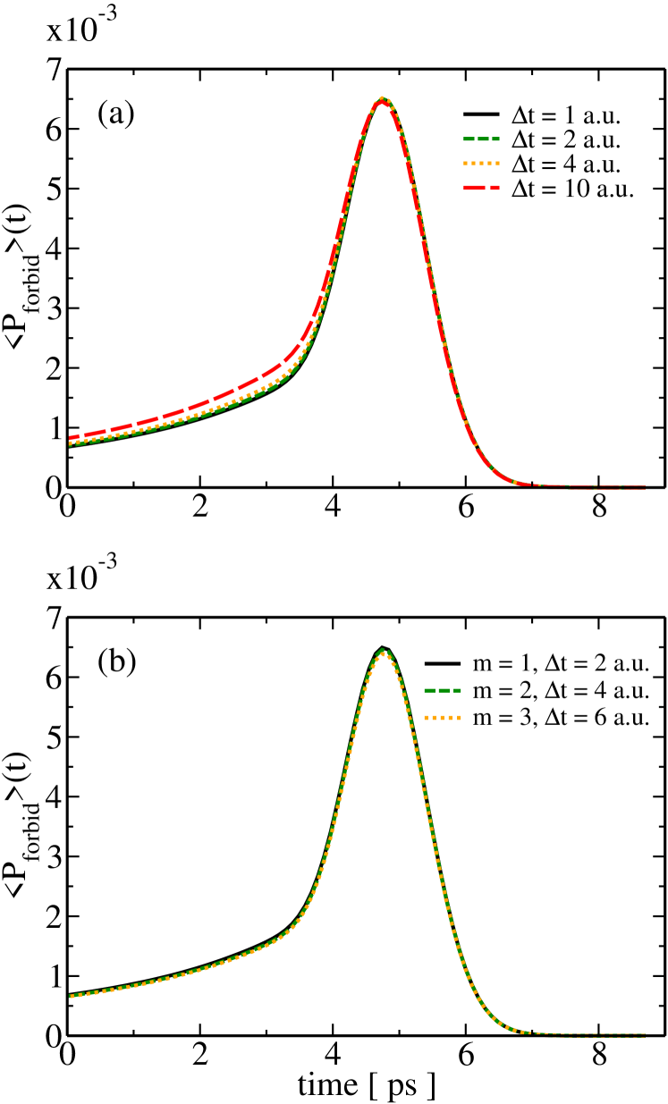
Figure 3: (color online) Normalized expectation value for the projector onto the forbidden subspace demonstrating the convergence of the inhomogeneous Chebychev propagator: (a) for first order solutions ($m=1$), convergence is lost by increasing $\Delta t$, (b) converged results for the largest possible time step at a given order $m$.

In first order, cf. Fig. 3a, the dynamics are found to be converged for time steps $\Delta t\leq 2\,$a.u. At larger time steps, deviations are observed, in particular at short times (occuring late for backward propagation). Dynamics with the largest possible time step at each order are shown in Fig. 3b.

order $m$	$\Delta t$	$N_{t}$	$N_{\mathrm{Cheby}}$	applications of $\boldsymbol{\mathsf{\hat{H}}}$	CPU time
1	$2\,$a.u.	180.000	6	$1.260.000$	$12\,$s
2	$4\,$a.u.	90.000	8	$900.000$	$11\,$s
3	$6\,$a.u.	60.000	10	$780.000$	$9\,$s

Table 1: CPU time required for one backward propagation to obtain converged solutions in first, second and third order for a total propagation time of $8\,$ps with equidistant time steps $\Delta t$. Also listed are the number of time steps, $N_{t}$, the number of times the Hamiltonian is applied and the number of terms in the Chebychev expansion, $N_{\mathrm{Cheby}}$.

In order to decide whether it is numerically more efficient to keep a low order demanding a small time step or to employ a higher order allowing for a larger time step, Table 1 compares the CPU time required to obtain converged solutions in first, second and third order. The number of applications of $\boldsymbol{\mathsf{\hat{H}}}$ includes both those occuring in the Chebychev recursion and those due to the additional terms in Eqs. (10-13). For example, for third order and $\Delta t=6\,$a.u., 10 Chebychev polynomials are sufficient to approximate $f_{3}(\boldsymbol{\mathsf{\hat{H}}})$ Eq. (13). Each time step then implies thirteen applications of $\boldsymbol{\mathsf{\hat{H}}}$, ten for the Chebychev recursion plus three for the additional terms (one for $|\lambda^{(1)}\rangle$ and two for $|\lambda^{(2)}\rangle$), cf. Eqs. (13) and (7). As can be seen in Table 1, in terms of CPU time, it is more efficient to employ a higher order solution. In the context of OCT calculations, in addition to saving computation time, a higher order propagator also allows for saving memory since the backward propagated wavefunction needs to be stored for each time step. An inherit limit to increasing the time step is, however, posed by the time-dependence of the Hamiltonian. Expressing the formal solution of the homogeneous time-dependent Schrödinger equation by the exponential, $e^{-i\boldsymbol{\mathsf{\hat{H}}}\Delta t}$, assumes $\boldsymbol{\mathsf{\hat{H}}}$ to be constant within the time interval $\Delta t$. In our example the upper limit at third order, $\Delta t=6\,$a.u., is due to the breakdown of this assumption for the forward propagated wavefunction, $|\varphi(t)\rangle$, entering the inhomogeneous term, $\lambda_{b}\boldsymbol{\mathsf{\hat{P}}}_{\mathrm{allow}}|\varphi(t)\rangle$.

In order to demonstrate that a higher-order solution for the inhomogeneous Schrödinger equation allows indeed for a large time step, we modify our example by invoking the rotating-wave approximation (RWA). This eliminates highly oscillatory terms from the field, $\epsilon(t)$, keeping only the time-dependence of the envelope which is several orders of magnitude slower. However, when increasing the time step and the order, numerical determination of the derivatives by FFT and multiplication in frequency domain breaks down, cf. Section III.2. Accurate numerical calculation of the time derivatives of the inhomogeneous term, $|\Phi(t)\rangle=\lambda_{b}\boldsymbol{\mathsf{\hat{P}}}_{\mathrm{allow}}|\varphi(t)\rangle$, is afforded by expanding $|\Phi(t)\rangle$ in Chebychev polynomials. The sampling points of the time grid then need to be chosen as the roots of the Chebychev polynomials, leading to non-equidistant time steps (dividing the time interval into equidistant time steps corresponds to a Fourier representation). Figure 4 and Table 2 illustrate the convergence behavior for a Hamiltonian with slow time-dependence.

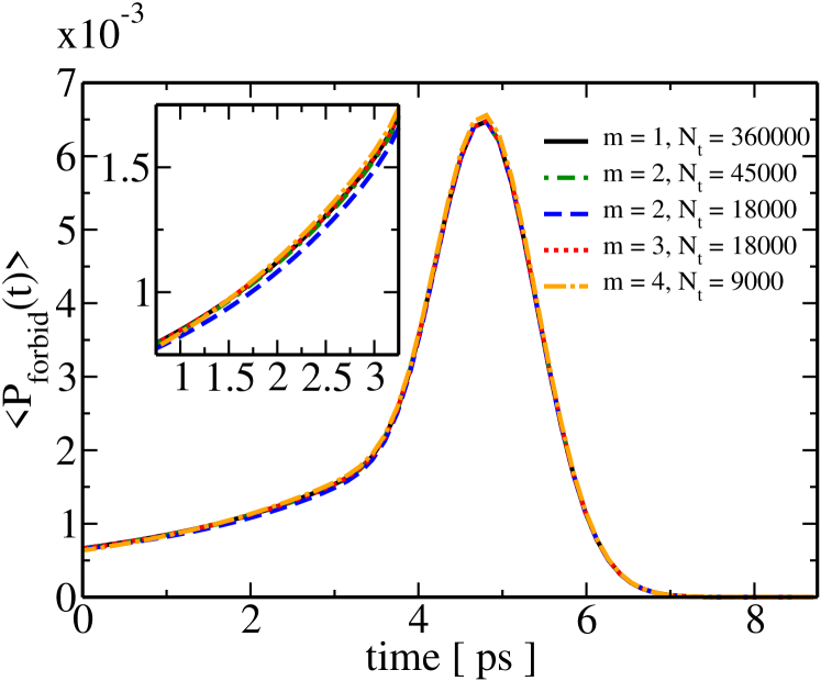
Figure 4: (color online) Normalized expectation value of the projector onto the forbidden subspace for a Hamiltonian with slow time-dependence (RWA) employing a non-equidistant time grid and calculating time derivatives in terms of Chebychev expansions for different orders $m$. Results are shown for the smallest possible number of time steps, $N_{t}$, at given order $m$ except for $m=2$, $N_{t}=18000$ (blue dashed line) which illustrates a non-converged case.

order $m$	$N_{t}$	$\Delta t_{\mathrm{max}}$	CPU time
2	$45.000$	$12.6\,$a.u.	$170\,$s
3	$18.000$	$31.4\,$a.u.	$69\,$s
4	$9.000$	$62.8\,$a.u.	$35\,$s

Table 2: CPU time required to obtain converged solutions in second, third and fourth order for a total propagation time of $8\,$ps with non-equidistant time steps. Also listed are the smallest possible number of sampling points for the time grid, $N_{t}$, and the corresponding maximum time step, $\Delta t_{\mathrm{max}}$.

All results in Fig. 4 are shown for the smallest possible number of time steps except the blue dashed line ($m=2$, $N_{t}=18.000$) which illustrates a non-converged case, cf. the deviation from the converged results at short times. The number of time steps can be significantly reduced by employing higher-order schemes. The evaluation of the derivatives by Chebychev expansion is, however, more costly, leading to overall larger computation times than in Table 1. It is obvious from Table 2 that this variant of the inhomogeneous Chebychev propagator will unfold its full power for a time-independent Hamiltonian that occurs e.g. in reactive scattering calculations where a very large time step together with a high-order scheme will be numerically most efficient. The fact that the permissible time step can be increased by employing a higher-order solution illustrates that inhomogeneous Chebychev propagator is based on a global representation.

V Application II: Control with a time-dependent target

In our second application, the operator occuring in the inhomogeneous term, $\boldsymbol{\mathsf{\hat{G}}}(t)$, is explicitly time-dependent.

V.1 Model

In principle it should be possible to prescribe by a laser pulse an arbitrary pathway that the quantum system should follow. To this end, OCT with a time-dependent target has to be employed SerbanPRA05 ; WerschnikJPB07 . In the total functional, Eq. (25), the final-time term then disappears, $J_{0}[\varphi_{T},\varphi_{T}^{*}]=0$, and the state- and time-dependent term becomes JoseMyPRA08

$$J_{b}[\varphi,\varphi^{\dagger}]=\int_{0}^{T}\lambda_{b}\langle\varphi(t)|\boldsymbol{\mathsf{\hat{G}}}(t)|\varphi(t)\rangle\,dt\,.$$ (32)

Maximization of $J_{b}$ corresponds to $\lambda_{b}\geq 0$ and fulfills the conditions for monotonic convergence JoseMyPRA08 .

A simple model comprising of five of the 33 levels of Section IV are taken to mimic a double $\Lambda$-system, cf. Fig. 5.

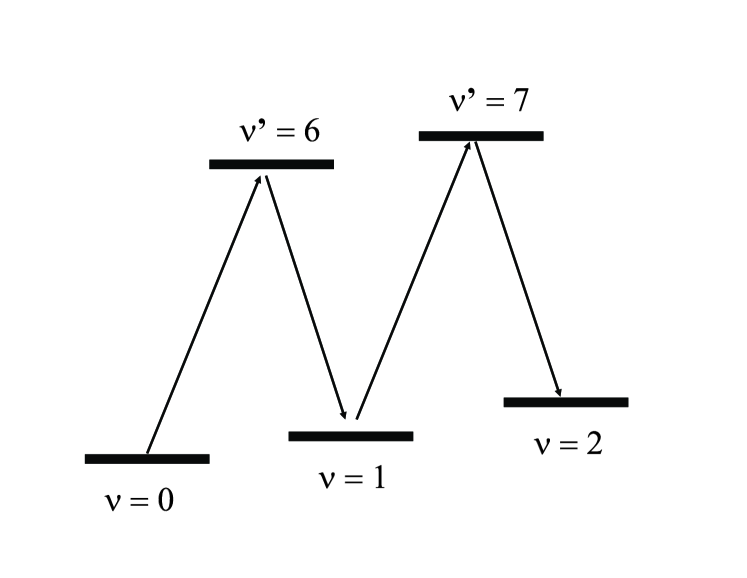
Figure 5: Prescribed ’trajectory’ for a time-dependent target: climbing up the ladder of a double $\Lambda$-system.

Initially all population is assumed to be in $v=0$, and at the final time the population in $v=2$ is to be maximal. Additionally, the time interval $[0,T]$ is divided into subintervals where the population of the intermediate levels $v^{\prime}=6$, $v=1$, and $v^{\prime}=7$, is maximized, i.e. we prescribe a ’trajectory’ where the ladder of the double $\Lambda$-system is sequentially climbed up. While this represents a simple toy model, it serves the purpose of illustrating the case where the operator of the inhomogeneous term of the Schrödinger equation, $\boldsymbol{\mathsf{\hat{G}}}(t)$, is explicitly time-dependent. The inhomogeneous equation for backward propagation reads,

$$\frac{d}{dt}|\psi(t)\rangle\,=\,-\frac{i}{\hbar}\,\boldsymbol{\mathsf{\hat{H}}}[\epsilon(t)]\,|\psi(t)\rangle\,+\,\lambda_{b}\boldsymbol{\mathsf{\hat{G}}}(t)|\varphi(t)\rangle\,,$$ (33)

with the “initial” condition

$$|\psi(t=T)\rangle\,=\,0\,.$$ (34)

Dividing the time interval $[0,T]$ into four subintervals, $0<T_{1}<T_{2}<T_{3}<T$, the target is defined as the projector onto $v^{\prime}=6$ in $[0,T_{1}]$, onto $v=1$ in $[T_{1},T_{2}]$, onto $v^{\prime}=7$ in $[T_{2},T_{3}]$ and onto $v=2$ in the subinterval $[T_{3},T]$,

$$\boldsymbol{\mathsf{\hat{G}}}(t) = |6\rangle\langle 6|\Theta(T_{1}-t)+\,$$ (35)

$$|1\rangle\langle 1|\Theta(t-T_{1})\Theta(T_{2}-t)+\,$$

$$|7\rangle\langle 7|\Theta(t-T_{2})\Theta(T_{3}-t)\,$$

$$|2\rangle\langle 2|\Theta(t-T_{3})\Theta(T-t)$$

with $\Theta(t)$ the Heaviside function. In order to avoid numerical problems due to discontinuities, $\Theta(t)$ is approximated by

$$\Gamma(t)=\frac{1}{1+e^{-kt}}\,,$$ (36)

where the parameter $k$ determines the steepness with which the target level changes. While for large values of $k$, the step function is recovered, small values of $k$ imply overlap in time of two different targets near the $T_{i}$, $i=1-3$. In the following $k$ is varied between $k=10^{-4}\,$a.u. and $k=10^{4}\,$a.u. The final time is set to $T=5.4\,$ps. The subintervals are taken to be of the same length, $T_{1}=1.35\,$ps, $T_{1}=2T_{1}$ and $T_{3}=3T_{1}$.

V.2 Results

The new propagator is tested for the iterative solution of the control equations with the time-dependent target. The guess field consists of a sequence of four $\pi$-pulses, one in each time interval. Figure 6 shows the evolution of the level populations using the optimized field for $k=10^{4}$.

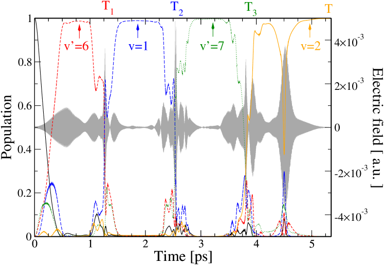
Figure 6: (color online) Time-dependent target: Time evolution of the level populations with an optimal field (shown in grey).

8

They follow by and large indeed the prescribed ’trajectory’. Population of levels other than the target one and fast oscillations in the populations are observed only when switching from one target to the next. The spectrum of the optimized field is shown in Fig. 7.

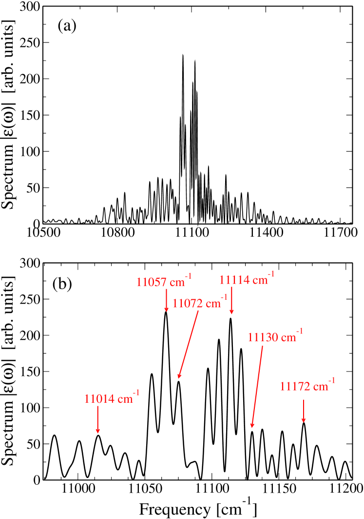
Figure 7: (color online) (a) Spectrum of the optimized field. (b) Detail of the spectrum ($\omega\in[10975\,\mathrm{cm}^{-1},11205\,\mathrm{cm}^{-1}]$). The numbers and arrows indicate the six main transition frequencies of the model, cf. Table 3.

The transition frequencies of our model, listed in Table 3 and indicated in Fig. 7b, are contained within the spectrum. Additional frequencies which do not correspond to the main transition frequencies are observed. They are attributed to the complexity of the optimal solution which may include beatings between levels, Stark shifts etc.

		0	1	2
6		$11130\,$	$11072\,$	$11014\,$
7		$11172\,$	$11114\,$	$11057\,$

Table 3: Transition frequencies in cm^-1 for the five levels employed as time-dependent target.

The improvement of the time-dependent target functional with the number of iterations is demonstrated in Fig. 8 for different values of the steepness parameter $k$.

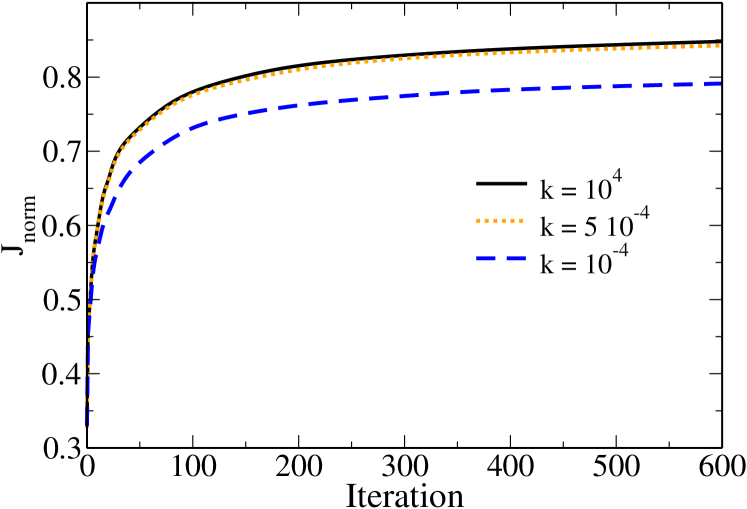
Figure 8: (color online) The renormalized functional $J_{b}$, cf. Eq. (32), as a function of the number of iterations for parameters $k$ corresponding to different overlaps in time of two targets.

Monotonic convergence is observed. However, the algorithm cannot reach 100%. We attribute this to the way the target is switched and overlap in time of different targets is created around the $T_{i}$, $i=1-3$. For large $k$ the changes in the target functional are almost instantaneous and cannot be followed by the dynamics, cf. the oscillations in the level populations in Fig. 6. However, at the same time, the targets do almost not overlap. This yields the highest value of the target functional, about 85%. For smaller values of $k$ the dynamics can follow more smoothly. However, the overlap between different targets is increased, i.e. contradictory objectives are asked at the same time. This decreases the value of the target functional to about 79%.

V.3 Convergence behavior

The convergence of the inhomogeneous Chebychev propagator is again analyzed with respect to the time step $\Delta t$ and to the order $m$. We restrict ourselves here to the case of equidistant time steps and calculation of the derivatives by FFT and multiplication in frequency domain. The convergence behavior is illustrated in Fig. 9 by the time evolution of the final target level ($v=2$) population.

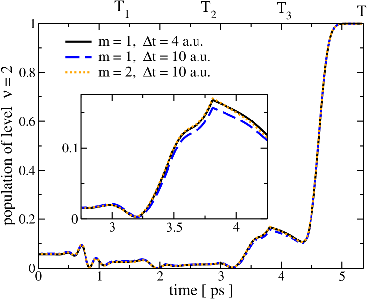
Figure 9: (color online) (a) Time-dependent population of the final target level $\nu\,=\,2$: Converged results in first and second orders for the largest possible time step (black solid and orange dotted lines). Also shown is a non-converged result in first order (blue dashed line) - the deviations from the converged solutions are evident in the insert.

Converged results are obtained for $\Delta t\leq 4\,$a.u. ($\Delta t\leq 10\,$a.u.) in first (second) order, i.e. a larger time step than in Section IV can be used. We attribute this to the much simpler model.

Table 4 compares the CPU time required to obtain converged solutions in first and second order.

order $m$	time step $\Delta t$	$N_{\mathrm{Cheby}}$	applications of $\boldsymbol{\mathsf{\hat{H}}}$	CPU time
1	$4\,$a.u.	8	$495.000$	$0.72\,$s
2	$10\,$a.u.	10	$264.000$	$0.62\,$s

Table 4: CPU time required to obtain converged solutions in first and second order for a total propagation time of $5.4\,$ps

The same conclusion is obtained as in Section IV, i.e it is more efficient to employ a higher order scheme.

Overall, no difference in the convergence behavior for time-dependent and time-independent operators in the inhomogeneous term, $\boldsymbol{\mathsf{\hat{G}}}(t)$ is found. This can be rationalized as follows: the convergence is determined by the fastest timescale of the dynamics, i.e. by the rapid oscillations of the field. The time-dependence of the projection operator introduces a time-dependence which is much slower and hence does not affect convergence.

VI Conclusions

A formal solution to the time-dependent inhomogeneous Schrödinger equation was derived based on an expansion of the inhomogeneous term. Three levels of Chebychev approximations are involved.

• The first one yields the Chebychev propagator where the argument of the Chebychev polynomials is the Hamiltonian. Truncating the expansion at the desired order $m$, the formal solution is subjected to a spectral representation with Chebychev polynomials. A propagation scheme similar to the standard Chebychev propagator for homogeneous Schrödinger equations is then obtained: Instead of $e^{-i\boldsymbol{\mathsf{\hat{H}}}\Delta t}$ a function $f_{m}(\boldsymbol{\mathsf{\hat{H}}})$ is expanded in Chebychev polynomials. For the exponential function, the expansion coefficients can be calculated analytically, for the function $f_{m}$they need to be obtained numerically. This is achieved by Fast Cosine Transformations, utilizing the definition of Chebychev polynomials in term of cosines.

• The second level expands the inhomogeneous state vector $|\Phi(t)\rangle$ in Chebychev polynomials within each short-time integration interval $[0,t]$. The argument of this expansion is the rescaled time $\bar{t}$ covering the interval. This Chebychev approximation is easily applied only if $|\Phi(t)\rangle$ is known analytically. If $|\Phi(t)\rangle$ is determined numerically on sampling points covering the global propagation time interval $[0,T]$, there are two choices. $|\Phi(t)\rangle$ needs to be interpolated to sampling points within $[0,t]$. In a simpler alternative, the Chebychev expansion is replaced by a Taylor expansion based on numerical derivatives at the beginning of each time step. This has been done for the present applications.

• The numerical calculation of the derivatives requires a third level of Chebychev approximation where the argument is the time $t$ covering the global propagation time interval $[0,T]$. This implies a non-equidistant time grid where the derivatives are evaluated according to the procedure described in Ref. Dunn96 . This expansion overcomes the numerical error introduced by non-zero boundary values of the inhomogeneous state vector $|\Phi(t)\rangle$ at $t=0$ and $t=T$. An alternative based on equidistant time steps employs Fast Fourier Transforms and multiplication in frequency domain. However, in that case the errors introduced at the boundary of the time grid build up. Therefore this scheme is limited to low order where only first or second derivatives are required.

An even more approximate solution to the time-dependent inhomogeneous Schrödinger equation is obtained by rewriting the formal solution explicitly in terms of a Taylor expansion. The propagator then consists of the standard exponential term plus time derivatives of the inhomogeneous terms. This approximation is numerically less efficient than the propagator for the full formal solution. Moreover, it may become instable in optimal control applications where the inhomogeneous term often is highly oscillatory and the numerical evaluation of derivatives by FFT becomes difficult. The main advantage of this propagation scheme lies in the fact that it requires very little modification of existing standard Chebychev propagation codes.

Both Chebychev propagation schemes were tested in two optimal control applications. OCT with a state-dependent constraint JoseMyPRA08 , e.g. maximizing population in an allowed subspace of the Hilbert space, yields a time-independent operator in the inhomogeneous term while an explicitly time-dependent operator is obtained in OCT with a time-dependent target KaiserJCP04 ; SerbanPRA05 ; KaiserCP06 ; WerschnikJPB07 . Convergence of the propagation schemes was demonstrated for both applications. The convergence behavior was studied in detail as a function of the order of the solution and the required number of time steps for a given overall propagation time. For applications with a fast time-dependence such as OCT, a low order scheme with a small time step and evaluation of the time derivatives by FFT was found to be the best choice. For applications with a slow time-dependence or time-independent Hamiltonians such as reactive scattering calculations where large time steps are permissible, a high-order scheme is numerically most efficient. This reflects that the propagation scheme is based on a global representation of the inhomogeneous term. It is this regime where the new propagator can best unfold its power.

The new Chebychev propagator provides a stable and accurate numerical solution to the time-dependent inhomogeneous Schrödinger equation. It is most efficient for high order and large time steps. Ideally an inherent time-dependence of the Hamiltonian should also be incorporated into the Chebychev scheme. This is the subject of a further study.

Appendix A Transformation to obtain $|\Phi^{(j)}\rangle$ from $|\bar{\Phi}_{j}\rangle$

When the solution of the inhomogeneous Schrödinger equation is based on the uniform approximation, a transformation linking the Chebychev expansion coefficients, $|\bar{\Phi}_{j}\rangle$, to the coefficients of the Taylor expansion, $|\Phi^{(j)}\rangle$, cf. Eq. (5), is required. In other words, given a vector $[A_{0},\ldots A_{m}]^{T}$ we want to compute the vector $[B_{0},\ldots B_{m}]^{T}$ such that

$$\sum_{k=0}^{m}A_{m,k}P_{k}(x)=\sum_{j=0}^{m}B_{m,j}\frac{x^{j}}{j!}\,,$$ (37)

i.e. we identify $|\bar{\Phi}_{k}\rangle$ and $|\Phi^{(j)}\rangle$ to $A_{m,k}$ and $B_{m,j}$ respectively. Let

$$P_{k}(x)=\sum_{j=0}^{k}C_{k,j}\frac{x^{j}}{j!}\,.$$ (38)

Since Chebychev polynomials obey the recursion relation,

$$P_{k+1}(x)=2xP_{k}(x)-P_{k-1}(x)\,,$$ (39)

we obtain

$$\sum_{j=0}^{k+1}C_{k+1,j}\frac{x^{j}}{j!}=2\sum_{j=0}^{k}C_{k,j}\frac{x^{j+1}}{j!}-\sum_{j=0}^{k-1}C_{k-1,j}\frac{x^{j}}{j!}\,,$$ (40)

or

$$\sum_{j=0}^{k+1}C_{k+1,j}\frac{x^{j}}{j!}=2\sum_{j=1}^{k+1}C_{k,j-1}\frac{x^{j}}{(j-1)!}-\sum_{j=0}^{k-1}C_{k-1,j}\frac{x^{j}}{j!}\,.$$ (41)

Hence, the $C$ coefficients satisfy

$$C_{k+1,0} = -C_{k-1,0}\,,$$

$$C_{k+1,j} = 2jC_{k,j-1}-C_{k-1,j}\quad,\quad 1\leq j\leq k-1$$

$$C_{k+1,k} = 2kC_{k,k-1}\,,$$

$$C_{k+1,k+1} = 2(k+1)C_{k,k}\,.$$ (42)

Based on this result we can compute the $B$ coefficients recursively,

$$B_{i+1,j} = B_{i,j}+A_{i+1,i+1}C_{i+1,j}\quad,\quad 1\leq j\leq i$$

$$B_{i+1,i+1} = A_{i,i}C_{i,i}\,,$$ (43)

for $1\leq i\leq m-1$ with

$$B_{0,0}=A_{0,0}\quad,\quad B_{1,0}=A_{1,0}\quad,\quad B_{1,1}=A_{1,1}\;.$$ (44)

Appendix B Proof of the equivalence of Eqs. (6) and (21)

It is shown by induction that the formal solution, Eq. (6), and Eq. (21) are equivalent. Writing Eqs. (6) and (21) for $m=1$, one obviously obtains in both cases the equation of the first order, Eq. (10). We assume that Eqs. (6) and (21) are equivalent in order $m-1$, i.e,

$$|\psi(t)\rangle_{(m-1)}=\sum_{j=0}^{m-2}\frac{t^{j}}{j!}|\lambda^{(j)}\rangle+\boldsymbol{\mathsf{\hat{F}}}_{m-1}|\lambda^{(m-1)}\rangle\,=e^{-i\boldsymbol{\mathsf{\hat{H}}}t}|\psi_{0}\rangle+\sum_{j=0}^{m-2}\boldsymbol{\mathsf{\hat{F}}}_{j+1}|\Phi^{(j)}\rangle\,,$$ (45)

let us now prove that they are equivalent in order $m$.

$$|\psi(t)\rangle_{(m)} = \sum_{j=0}^{m-1}\frac{t^{j}}{j!}|\lambda^{(j)}\rangle+\boldsymbol{\mathsf{\hat{F}}}_{m}|\lambda^{(m)}\rangle\,$$ (46)

$$= \sum_{j=0}^{m-2}\frac{t^{j}}{j!}|\lambda^{(j)}\rangle+\frac{t^{m-1}}{(m-1)!}|\lambda^{(m-1)}\rangle+\boldsymbol{\mathsf{\hat{F}}}_{m}\left((-i\boldsymbol{\mathsf{\hat{H}}})|\lambda^{(m-1)}\rangle+|\Phi^{(m-1)}\rangle\right)\,$$

$$= \sum_{j=0}^{m-2}\frac{t^{j}}{j!}|\lambda^{(j)}\rangle+\boldsymbol{\mathsf{\hat{F}}}_{m}|\Phi^{(m-1)}\rangle+\left(\boldsymbol{\mathsf{\hat{F}}}_{m}(-i\boldsymbol{\mathsf{\hat{H}}})+\leavevmode\hbox{\small 1\kern-3.3pt\normalsize 1}\frac{t^{m-1}}{(m-1)!}\right)|\lambda^{(m-1)}\rangle$$

We continue by showing that $\boldsymbol{\mathsf{\hat{F}}}_{m-1}=\boldsymbol{\mathsf{\hat{F}}}_{m}(-i\boldsymbol{\mathsf{\hat{H}}})+\leavevmode\hbox{\small 1\kern-3.3pt\normalsize 1}\frac{t^{m-1}}{(m-1)!}$,

$$\boldsymbol{\mathsf{\hat{F}}}_{m}(-i\boldsymbol{\mathsf{\hat{H}}})+\leavevmode\hbox{\small 1\kern-3.3pt\normalsize 1}\frac{t^{m-1}}{(m-1)!} = (-i\boldsymbol{\mathsf{\hat{H}}})^{-(m-1)}\left(e^{-i\boldsymbol{\mathsf{\hat{H}}}t}-\sum_{j=0}^{m-2}\frac{(-i\boldsymbol{\mathsf{\hat{H}}}t)^{j}}{j!}-\frac{(-i\boldsymbol{\mathsf{\hat{H}}}t)^{m-1}}{(m-1)!}\right)+\leavevmode\hbox{\small 1\kern-3.3pt\normalsize 1}\frac{t^{m-1}}{(m-1)!}\,$$

$$= (-i\boldsymbol{\mathsf{\hat{H}}})^{-(m-1)}\left(e^{-i\boldsymbol{\mathsf{\hat{H}}}t}-\sum_{j=0}^{m-2}\frac{(-i\boldsymbol{\mathsf{\hat{H}}}t)^{j}}{j!}\right)-(-i\boldsymbol{\mathsf{\hat{H}}})^{-(m-1)}\frac{(-i\boldsymbol{\mathsf{\hat{H}}}t)^{m-1}}{(m-1)!}+\leavevmode\hbox{\small 1\kern-3.3pt\normalsize 1}\frac{t^{m-1}}{(m-1)!}\,$$

$$= (-i\boldsymbol{\mathsf{\hat{H}}})^{-(m-1)}\left(e^{-i\boldsymbol{\mathsf{\hat{H}}}t}-\sum_{j=0}^{m-2}\frac{(-i\boldsymbol{\mathsf{\hat{H}}}t)^{j}}{j!}\right)-\leavevmode\hbox{\small 1\kern-3.3pt\normalsize 1}(\frac{t^{m-1}}{(m-1)!}-\frac{t^{m-1}}{(m-1)!})\,$$

$$= (-i\boldsymbol{\mathsf{\hat{H}}})^{-(m-1)}\left(e^{-i\boldsymbol{\mathsf{\hat{H}}}t}-\sum_{j=0}^{m-2}\frac{(-i\boldsymbol{\mathsf{\hat{H}}}t)^{j}}{j!}\right)=\boldsymbol{\mathsf{\hat{F}}}_{m-1}\,.$$

Equation (46) thus becomes

$$|\psi(t)\rangle_{(m)}=\sum_{j=0}^{m-2}\frac{t^{j}}{j!}|\lambda^{(j)}\rangle+\boldsymbol{\mathsf{\hat{F}}}_{m-1}|\lambda^{(m-1)}\rangle+\boldsymbol{\mathsf{\hat{F}}}_{m}|\Phi^{(m-1)}\rangle\,.$$

Making use of our assumption, Eq. (45), we obtain

$$|\psi(t)\rangle_{(m)} = e^{-i\boldsymbol{\mathsf{\hat{H}}}t}|\psi_{0}\rangle+\sum_{j=0}^{m-2}\boldsymbol{\mathsf{\hat{F}}}_{j+1}|\Phi^{(j)}\rangle\ +\boldsymbol{\mathsf{\hat{F}}}_{m}|\Phi^{(m-1)}\rangle$$

$$= e^{-i\boldsymbol{\mathsf{\hat{H}}}t}|\psi_{0}\rangle+\sum_{j=0}^{m-1}\boldsymbol{\mathsf{\hat{F}}}_{j+1}|\Phi^{(j)}\rangle\,.$$

This concludes the proof.

Appendix C Algorithm of the symmetrical method

The symmetrical method of Ref. JoseMyPRA08 is based on the formal integration of the inhomogeneous time-dependent Schrödinger equation, Eq. (3),

$$|\psi(t)\rangle=e^{-i\boldsymbol{\mathsf{\hat{H}}}t}|\psi(0)\rangle+e^{-i\boldsymbol{\mathsf{\hat{H}}}t}\int_{0}^{t}e^{i\boldsymbol{\mathsf{\hat{H}}}\tau}|\bar{\Phi}(\tau)\rangle d\tau\,.$$ (47)

Assuming $|\bar{\Phi}(\tau)\rangle$ to be constant in $[0,t]$ and taking its value to be

$$|\bar{\Phi}(\tau)\rangle=\frac{|\Phi(0)\rangle+|\Phi(t)\rangle}{2}\qquad\forall\tau\in[0,t]\,,$$ (48)

the integral in Eq. (47) can easily be computed and we obtain

$$|\psi(t)\rangle\approx e^{-i\boldsymbol{\mathsf{\hat{H}}}t}|\psi(0)\rangle+(-i\boldsymbol{\mathsf{\hat{H}}})^{-1}\left(e^{-i\boldsymbol{\mathsf{\hat{H}}}t}-\leavevmode\hbox{\small 1\kern-3.3pt\normalsize 1}\right)|\bar{\Phi}(0)\rangle\,.$$ (49)

This solution is formally equivalent to the first order of the Chebychev propagator, cf. Eq (10). However, the evaluation of $|\psi(t)\rangle$ proceeds differently in the symmetrical method and the first order Chebychev propagator. The latter subjects Eq. (49) to a spectral approximation. It only requires a representation of the Hamiltonian such that its action on a state vector can be evaluated. A numerically very efficient representation is based on the Fourier grid where evaluation of $\boldsymbol{\mathsf{\hat{H}}}|\psi\rangle$ scales as $O(N\log N)$ with $N$ the number of grid points. The symmetrical method diagonalizes $\boldsymbol{\mathsf{\hat{H}}}(t)$ at each time step in order to directly employ Eq. (49). Since diagonalization scales as $O(N^{3})$, where $N$ is the dimension of the Hilbert space, this is feasible only for sufficiently small $N$.

References

- (1) D. Neuhauser, M. Baer, R. S. Judson, and D. J. Kouri, Comput. Phys. Comm. 63, 460 (1991).
- (2) D. Neuhauser, Chem. Phys. Lett. 200, 173 (1992).
- (3) A. Kaiser and V. May, J. Chem. Phys. 121, 2528 (2004).
- (4) I. Şerban, J. Werschnik, and E. K. U. Gross, Phys. Rev. A 71, 053810 (2005).
- (5) A. Kaiser and V. May, Chem. Phys. 320, 95 (2006).
- (6) J. Werschnik and E. K. U. Gross, J. Phys. B 40, R175 (2007).
- (7) J. P. Palao, R. Kosloff, and C. P. Koch, Phys. Rev. A 77, 063412 (2008).
- (8) D. Neuhauser and M. Baer, J. Chem. Phys. 91, 4651 (1989).
- (9) W. Zhu, J. Botina, and H. Rabitz, J. Chem. Phys. 108, 1953 (1998).
- (10) J. P. Palao and R. Kosloff, Phys. Rev. A 68, 062308 (2003).
- (11) Y. Ohtsuki, G. Turinici, and H. Rabitz, J. Chem. Phys. 120, 5509 (2004).
- (12) R. Kosloff, J. Phys. Chem. 92, 2087 (1988).
- (13) R. Kosloff, Annu. Rev. Phys. Chem. 45, 145 (1994).
- (14) H. Tal-Ezer and R. Kosloff, J. Chem. Phys. 81, 3967 (1984).
- (15) R. Baer, Phys. Rev. A 62, 063810 (2000).
- (16) D. Dunn, Comput. Phys. Comm. 96, 10 (1996).
- (17) S. J. Park, S. W. Suh, Y. S. Lee, and G. H. Jeung, J. Molec. Spec. 207, 129 (2001).