On analyticity with respect to the replica number in random energy models I: an exact expression of the moment of the partition function

Abstract

We provide an exact expression of the moment of the partition function for random energy models of finite system size, generalizing an earlier expression for a grand canonical version of the discrete random energy model presented by the authors in Prog. Theor. Phys. 111, 661 (2004). The expression can be handled both analytically and numerically, which is useful for examining how the analyticity of the moment with respect to the replica numbers, which play the role of powers of the moment, can be broken in the thermodynamic limit. A comparison with a replica method analysis indicates that the analyticity breaking can be regarded as the origin of the one-step replica symmetry breaking. The validity of the expression is also confirmed by numerical methods for finite systems.

1 Introduction

The replica method (RM) is one of the few analytical techniques available for dealing with disordered systems [1, 2]. In general, RM can be regarded as a scheme for evaluating the generating function

$$\phi_{N}(n)=\frac{1}{N}\log\left\langle Z^{n}\right\rangle,$$ (1)

for real number $n\in\mathbb{R}\ (\mbox{or complex}\ \mathbb{C})$, where $Z$ and $\left\langle\cdots\right\rangle$ represent the partition function and the average over the quenched randomness that governs the objective system, respectively. Unfortunately, direct evaluation of eq. (1) is difficult in general. In statistical mechanics, the system size $N$ is in most cases assumed to be infinitely large, which often makes the analysis possible for $n=1,2,\ldots\in\mathbb{N}$. Therefore, RM in statistical mechanics usually first evaluates eq. (1) for $n\in\mathbb{N}$ in the limit $N\to\infty$ as

$$\phi(n)=\lim_{N\to\infty}\phi_{N}(n),$$ (2)

and then analytically continue the expression from $n\in\mathbb{N}$ to $n\in\mathbb{R}$.

This procedure generally includes at least two mathematical problems, although it was recently proved for several examples that the solutions obtained by RM are mathematically correct [3, 4]. The first problem concerns the uniqueness of the analytic continuation from $n\in\mathbb{N}$ to $n\in\mathbb{R}$. Even if all values of $\phi_{N}(n)$ are provided for $n=1,2,\ldots$, in general, it is not possible to determine the analytical continuation from $n\in\mathbb{N}$ to $n\in\mathbb{R}\ ({\rm or}\ \mathbb{C})$ uniquely. Carlson’s theorem guarantees that the continuation in the right half complex plane is unique if the growth rate of $\left|\left\langle Z^{n}\right\rangle^{1/N}\right|$ is upper-bounded by $O(e^{\pi|n|})$ [5]. However, this sufficient condition is not satisfied even in the case of the famous Sherrington–Kirkpatrick (SK) model that describes a fully connected Ising spin glass system [6], for which $\left|\left\langle Z^{n}\right\rangle^{1/N}\right|$ scales as $O(e^{C|n|^{2}})$, where $C$ is a certain constant. van Hemmen and Palmer conjectured that this might be related to the failure of the replica symmetric (RS) solution of the SK model at low temperatures, although further exploration in this direction is difficult [7].

The second issue is the possible breaking of the analyticity of $\phi(n)$. Even if the uniqueness of the analytic continuation from $n\in\mathbb{N}$ to $n\in\mathbb{R}\ ({\rm or}\ \mathbb{C})$ is guaranteed for $\phi_{N}(n)$ of finite $N$, the analyticity of $\phi(n)=\lim_{N\to\infty}\phi_{N}(n)$ can be broken. This implies that if the analyticity breaking occurs at a certain point $n=n_{c}<1$, the analytically continued expression based on $\phi(n)$ will lead to an incorrect solution for $n<n_{c}$. In an earlier study, the authors developed an exact expression of $\left\langle Z^{n}\right\rangle$ for a grand canonical version of the discrete random energy model (GCDREM) [8, 9] of finite system size [10]. The expression indicates that the speculated scenario does occur in this model as $N\to\infty$. In addition, the model satisfies the sufficient condition of Carlson’s theorem, guaranteeing the uniqueness of the analytical continuation for finite $N$. These points imply that the analyticity breaking with respect to the replica number $n$ is the origin of the one-step replica symmetry breaking (1RSB) observed in GCDREM. However, as GCDREM is a relatively unfamiliar model, the obtained result may be regarded as anomalistic and therefore might be taken as being less significant.

The purpose of this paper is to address this view. More precisely, we develop an exact expression of $\left\langle Z^{n}\right\rangle$ that is applicable to generic random energy models (REMs) [11] of finite system size. The expression, which is a generalization of that developed for GCDREM, indicates that analyticity breaking with respect to the replica number occurs in standard REMs as well and is the origin of 1RSB.

This paper is organized as follows. In the next section, we introduce the model. In order to guarantee the uniqueness of analytical continuation, we will mainly consider the canonical version of the discrete random energy model (CDREM). However, a similar approach is also applicable for standard continuous REM, although the uniqueness of the analytical continuation from $n\in\mathbb{N}$ to $n\in\mathbb{C}$ is not guaranteed by Carlson’s theorem. This is shown in A. In section 3, the main part of the paper, an exact expression of $\left\langle Z^{n}\right\rangle$ is developed. In section 4, the developed expression is used to examine how the analyticity of $\left\langle Z^{n}\right\rangle$ can be broken as $N\to\infty$. The utility of the expression for assessing the moment of REMs of finite size is also shown. The final section is devoted to a summary.

2 Model definition

The canonical discrete random energy model (CDREM), which we will focus on here, is defined as follows. Suppose that $N$ and $M$ are natural numbers where $\alpha=M/N$. The energy for each of $2^{N}$ states $A=1,2,\ldots,2^{N}$ is determined as an independent sample from an identical distribution

$$P(E)=2^{-M}\left(\begin{array}[]{c}M\\ \frac{1}{2}M+E\end{array}\right),$$ (5)

where $E$ is limited to $-M/2,-M/2+1,\ldots,M/2$. We denote a set of sampled energy values as $\{\epsilon_{A}\}$. For each realization of $\{\epsilon_{A}\}$, the partition function is defined as

$$Z = \sum_{A=1}^{2^{N}}\exp(-\beta\epsilon_{A}),$$ (6)

where $\beta=T^{-1}>0$ denotes the inverse temperature. Our main objective is to develop an expression of $\left\langle Z^{n}\right\rangle$, the evaluation of which is computationally feasible for $\forall{N},\forall{M}$ and $\forall{n}\in\mathbb{C}$, where $\left\langle\cdots\right\rangle$, in this case, represents the average with respect to $\{\epsilon_{A}\}$.

Before proceeding further, it is worth explaining why this model has been selected. A distinctive property of this model is that the possible energy values are lower-bounded by $-M/2$, which makes it possible to upper-bound the absolute value of a modified moment as

$$\left|\left\langle\left(e^{-\beta M/2}Z\right)^{n}\right\rangle^{1/N}\right|\leq\left\langle\left(e^{-\beta M/2}Z\right)^{{\rm Re}(n)}\right\rangle^{1/N}=\left\langle\left(\sum_{A=1}^{2^{N}}e^{-\beta(M/2+\epsilon_{A})}\right)^{{\rm Re}(n)}\right\rangle^{1/N}$$ (7)

$$\leq\left\langle\left(\sum_{A=1}^{2^{N}}1\right)^{{\rm Re}(n)}\right\rangle^{1/N}=2^{{\rm Re}(n)}<O(e^{\pi|n|}),$$ (8)

for any finite $N$. Consider an analytic function $\Psi(n;N)$ which satisfies the condition $|\Psi(n;N)|<O(e^{\pi|n|})$. Carlson’s theorem ensures that if $\left|\Psi(n;N)-\left\langle\left(e^{-\beta M/2}Z\right)^{n}\right\rangle^{1/N}\right|=0$ holds for $n=0,1,2\ldots$, $\Psi(n;N)$ is identical to $\left\langle\left(e^{-\beta M/2}Z\right)^{n}\right\rangle^{1/N}$ over the right half complex plane of $n$. The identity for $n=0$ trivially holds if $\Psi(0;N)=1$. Since $e^{-\beta M/2}$ is a non-vanishing constant and $\left\langle\left(e^{-\beta M/2}Z\right)^{n}\right\rangle^{1/N}$ is a single-valued function, this implies that the analytical continuation of $\left\langle Z^{n}\right\rangle^{1/N}$ from $n=1,2,\ldots$ to $n\in\mathbb{C}$ is uniquely determined in this model as long as $N$ is finite. This property is useful for examining intrinsic mathematical problems of RM because we can exclude the possibility of multiple analytical continuations when certain anomalous behavior is observed for $\left\langle Z^{n}\right\rangle$. This is the main reason why we have selected CDREM as the objective system in the current paper.

The technique developed in the next section is also applicable to generic REMs, as shown in A. Unfortunately, we cannot use Carlson’s theorem for guaranteeing the uniqueness of the analytical continuation for the original continuous REM [11], since $\left|\left\langle Z^{n}\right\rangle^{1/N}\right|$ is not upper-bounded by $e^{\pi|n|}$. However, the analysis in A indicates that the behavior of the continuous REM in the thermodynamic limit is qualitatively the same as that of CDREM; in both systems, $\phi(n)$ for $n=1,2,\ldots$ is described by either of two replica symmetric solutions one of which is proportional to $n$ while the other is nonlinear with respect to $n$, and the replica symmetry breaking solution bifurcates from the nonlinear solution at a certain critical number $0<n_{c}<1$ for $n<n_{c}$ when the temperature is sufficiently low. This implies that, for a wide class of random energy models, the origin of replica symmetry breaking is not the multiple possibilities of analytical continuation but the analyticity breaking with respect to the replica number that occurs in the thermodynamic limit.

3 Exact expression of $\left\langle Z^{n}\right\rangle$

The expression of the partition function

$$Z=\sum_{A=1}^{2^{N}}\exp(-\beta\epsilon_{A})=\sum_{i=0}^{M}n_{i}\exp(-\beta E_{i})=\omega^{-\frac{M}{2}}\sum_{i=0}^{M}n_{i}\omega^{i}\ \ (\omega\equiv e^{-\beta}),$$ (9)

is the basis of our analysis, where $n_{i}$ $(i=0,1,\ldots,M)$ represents the number of states with energy $E=i-M/2$. A remarkable property of DREM is that the probability distribution of $\{n_{i}\}$ has a feasible form as a multinomial distribution

$$P(\{n_{i}\})=\delta_{\sum_{i=0}^{M}n_{i},2^{N}}\frac{2^{N}!}{n_{0}!\cdots n_{M}!}\prod_{i=0}^{M}\{P(E_{i})\}^{n_{i}},$$ (10)

where $\delta_{m,n}=1$ if $m=n$ and $0$ otherwise. This makes it possible to assess the moments $\left\langle Z^{n}\right\rangle$ directly from $\{n_{i}\}$ without referring to the full energy configuration $\{\epsilon_{A}\}$, yielding

$$\left\langle Z^{n}\right\rangle = \sum_{n_{0}=0}^{\infty}\sum_{n_{1}=0}^{\infty}\cdots\sum_{n_{M}=0}^{\infty}P(\{n_{i}\})Z^{n}$$ (12)

$$= \sum_{n_{0}=0}^{\infty}\sum_{n_{1}=0}^{\infty}\cdots\sum_{n_{M}=0}^{\infty}\{P(E_{0})\}^{n_{0}}\{P(E_{1})\}^{n_{1}}\cdots\{P(E_{M})\}^{n_{2}}\$$

$$\times\delta_{\sum_{i=0}n_{i},2^{N}}\frac{2^{N}!}{n_{0}!\cdots n_{M}!}\ Z^{n}.$$

Two identities are useful for evaluating eq. (12):

$$c^{n}=\frac{\int_{H}(-\rho)^{-n-1}e^{-c\rho}d\rho}{\tilde{\Gamma}(-n)},\ \ (c>0,\tilde{\Gamma}(n)\equiv-2{\rm i}\sin n\pi\Gamma(n)),$$ (13)

and

$$\delta_{m,n}=\frac{1}{2\pi{\rm i}}\oint z^{m-n-1}dz,$$ (14)

where ${\rm i}=\sqrt{-1}$. In eq. (13), $\Gamma(z)={\rm i}/(2\sin z\pi)\int_{H}(-\rho)^{z-1}e^{-\rho}d\rho$ represents the Gamma function and the integration contour $H$ is provided as shown in figure 1. The integration contour of eq. (14) is a single closed loop surrounding the origin. Inserting eqs. (13) and (14) into eq. (12) yields

$$\left\langle Z^{n}\right\rangle = \sum_{n_{0}=0}^{\infty}\sum_{n_{1}=0}^{\infty}\cdots\sum_{n_{M}=0}^{\infty}\{P(E_{0})\}^{n_{0}}\{P(E_{1})\}^{n_{1}}\cdots\{P(E_{M})\}^{n_{2}}\ \frac{2^{N}!}{n_{0}!\cdots n_{M}!}\$$

$$\frac{\omega^{-\frac{nM}{2}}}{\tilde{\Gamma}(-n)}\int_{H}d\rho(-\rho)^{-n-1}e^{-(\sum_{i=0}^{M}n_{i}\omega^{i})\rho}\frac{1}{2\pi{\rm i}}\oint dzz^{\sum_{i=0}^{M}n_{i}-2^{N}-1}$$

$$= \frac{\omega^{-\frac{nM}{2}}}{\tilde{\Gamma}(-n)}\int_{H}d\rho(-\rho)^{-n-1}\frac{(2^{N})!}{2\pi{\rm i}}\oint dzz^{-2^{N}-1}\left(\sum_{n_{0}=0}^{\infty}\frac{1}{n_{0}!}\{zP(E_{0})e^{-\rho}\}^{n_{0}}\right)$$

$$\left(\sum_{n_{1}=0}^{\infty}\frac{1}{n_{1}!}\{zP(E_{1})e^{-\omega\rho}\}^{n_{1}}\right)\cdots\left(\sum_{n_{M}=0}^{\infty}\frac{1}{n_{M}!}\{zP(E_{M})e^{-\omega^{M}\rho}\}^{n_{M}}\right)$$

$$= \frac{\omega^{-\frac{nM}{2}}}{\tilde{\Gamma}(-n)}\int_{H}d\rho(-\rho)^{-n-1}\frac{(2^{N})!}{2\pi{\rm i}}\oint dzz^{-2^{N}-1}e^{z\sum_{i=0}^{M}P(E_{i})e^{-\omega^{i}\rho}}.$$ (16)

Finally, applying the residue theorem to the integration with respect to $z$, we obtain

$$\left\langle Z^{n}\right\rangle = \frac{\omega^{-\frac{nM}{2}}}{\tilde{\Gamma}(-n)}\int_{H}d\rho(-\rho)^{-n-1}\left(\sum_{i=0}^{M}P(E_{i})e^{-\omega^{i}\rho}\right)^{2^{N}},$$ (17)

which exactly holds for any complex value of $n$. This is the main result of this paper.

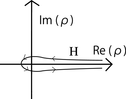
Figure 1: Integration contour.

Several points are noteworthy here. The first issue is a relation to an earlier study. In ref. [12], Gardner and Derrida provided an expression somewhat similar to eq. (17) for non-integer moments of the partition function of the continuous REM. Actually, the present expression of eq. (17) can be regarded as a generalization of eq. (7) of ref. [12], for which, however, tractability for finite $N$ is not emphasized. The link of the two expressions is shown in A. The second is the computational cost for evaluating eq. (17). For each $\rho\in\mathbb{C}$, the integrand of eq. (17) can be evaluated with $O(N)$ computations provided $\alpha=M/N\sim O(1)$. On the other hand, the length of the integration contour $H$ is infinite, which may seem an obstacle for the numerical evaluation. However, for relatively large $N$, the integrand rapidly vanishes on the contour $H$ as $|\rho|\to\infty$, guaranteeing that numerical deviation is practically negligible even if we approximate $H$ by a path of a finite length. Therefore, eq. (17) can be evaluated with a feasible computational cost. The third point is the similarity to an approach in information theory sometimes termed the method of types [13]. In this method, the performance of various codes consisting of exponentially many codewords is evaluated by classifying possible events when the codes are randomly generated by varieties of empirical distributions, termed types. The key to this method is accounting for the fact that the number of types grows only polynomially with respect to the code length while the number of the codewords increases exponentially. As a consequence, the relative weight of the types concentrates at a certain typical value at an exponentially fast rate, which considerably simplifies the performance analysis. In the current case, the set of occupation numbers $\{n_{i}\}$ is analogous to the types in information theory. However, in spite of this analogy, objective quantities are usually evaluated by upper- and lower-bounding schemes in information theory. Therefore, the technique developed in the present paper may serve as a novel scheme for analyzing various codes in information theory. The final issue relates to the relationship to a model examined in an earlier study. In ref. [10], the authors offered a formula similar to eq. (17) for a grand canonical version of the discrete random energy model (GCDREM). Unlike CDREM, GCDREM is defined by independently generating the occupation number $n_{i}$ of each energy level from the beginning. In the present framework, this can be characterized by a factorizable distribution of $\{n_{i}\}$,

$$P(\{n_{i}\})=e^{-2^{N}}\prod_{i=0}^{M}\frac{\left(-P(E_{i})2^{N}\right)^{n_{i}}}{n_{i}!},$$ (18)

which offers a feasible expression

$$\left\langle Z^{n}\right\rangle=\frac{\omega^{-\frac{nM}{2}}}{\tilde{\Gamma}(-n)}\int_{H}d\rho(-\rho)^{-n-1}\exp{[-\sum_{i=0}^{M}(1-e^{-\omega^{i}\rho})P(E_{i})2^{N}]}.$$ (19)

This is the counterpart of eq. (17). Since the distributions of $n_{i}$ are independent, the derivation of eq. (19) is easier than that of eq. (17). In GCDREM, the total number of states ${\cal N}=\sum_{i=0}^{M}n_{i}$ fluctuates from sample to sample as $n_{i}$ is independently generated at each energy level. The ratio between its standard deviation and expectation vanishes as $2^{-N/2}$ and therefore the effect of the statistical fluctuation is practically negligible when $N$ is reasonably large. Nevertheless, eq. (18) implies that an ill-posed sample $n_{i}=0$ $(i=0,1,\ldots,M)$ can be generated with a probability $2^{-N}$, which is not adequate for representing REMs of small system size. Therefore, the development of eq. (17) beyond eq. (19) is important for REMs of finite size.

4 Applications

In this section, we demonstrate the utility of the developed expression (17) by considering two applications.

4.1 Thermodynamic limit and breaking of analyticity

RM indicates that CDREM exhibits the following behavior in the thermodynamic limit $N,M\to\infty$ keeping $\alpha=M/N$ finite. For details, see B.

Under the RS ansatz, RM yields two solutions

$$\phi_{\rm RS1}(n)=n\left(\log 2+\alpha\log\left(\cosh\left(\frac{\beta}{2}\right)\right)\right),$$ (20)

and

$$\phi_{\rm RS2}(n)=\log 2+\alpha\log\left(\cosh\left(\frac{n\beta}{2}\right)\right).$$ (21)

For $\forall{\alpha}$ and $\forall{\beta}$, these solutions agree at $n=1$. Let us denote a critical inverse temperature as

$$\beta_{c}=\left\{\begin{array}[]{ll}\infty,&\alpha\leq 1\cr\log\left(1-h_{2}^{-1}(1-\alpha^{-1})\right)-\log\left(h_{2}^{-1}(1-\alpha^{-1})\right),&\alpha>1\end{array}\right.,$$ (24)

where $h_{2}^{-1}(y)$ is the inverse function of the binary entropy $h_{2}(x)=-x\log_{2}(1-x)-(1-x)\log_{2}(1-x)$ for $0<x<1/2$. For $\beta<\beta_{c}$, $\phi(n)$ can be described by $\phi_{\rm RS1}(n)$ and $\phi_{\rm RS2}(n)$. More precisely, there exists $\exists{n_{\rm RS}}>1$ such that $\phi(n)=\phi_{\rm RS2}(n)$ for $n>n_{\rm RS}$ and $\phi(n)=\phi_{\rm RS1}(n)$ for $n<n_{\rm RS}$. On the other hand, for $\beta>\beta_{c}$, $\phi(n)$ cannot be entirely covered by the RS solutions. In this “low temperature” phase, $\phi(n)=\phi_{\rm RS2}(n)$ holds for $n>n_{c}=\beta_{c}/\beta$. However, this solution becomes inadequate for $n<n_{c}$ since the convexity condition $\left(\partial/\partial n\right)\left(n^{-1}\phi_{\rm RS2}(n)\right)\geq 0$ is not satisfied. Therefore, we have to construct a novel solution for $n<n_{c}$ taking the breaking of replica symmetry into account, which provides the 1RSB solution

$$\phi_{\rm 1RSB}(n)=\frac{n\alpha\beta}{2}\tanh\frac{\beta_{c}}{2}.$$ (25)

The behavior of $\phi(n)$ is shown in figure 2.

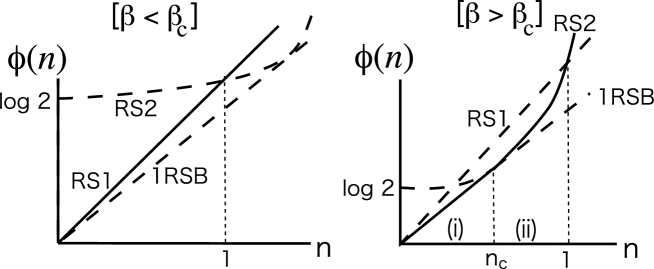
Figure 2: Behavior of $\phi(n)$ predicted by RM.

As long as $N$ is finite, $\phi_{N}(n)$ is generally analytic with respect to $n$ and Carlson’s theorem guarantees the uniqueness of the analytical continuation from $n\in\mathbb{N}$ to $n\in\mathbb{C}$ for $\phi_{N}(n)$ of CDREM. This implies that the transitions between multiple solutions mentioned above are highly likely to be due to the breaking of analyticity that possibly occurs in the limit $\phi(n)=\lim_{N\to\infty}\phi_{N}(n)$. The expression of eq. (17) can be used to examine the origin of such potential analyticity breaking.

We here focus on the breaking for the transition between $\phi_{\rm RS2}(n)$ and $\phi_{\rm 1RSB}(n)$, which can be regarded as the origin of 1RSB. For this purpose, we assume $\alpha>1$ and $\beta>\beta_{c}$, and consider only the region $n<1$ in which $n_{c}=\beta_{c}/\beta<1$ is included. Under such conditions, integration by parts transforms eq. (17) to

$$\left\langle Z^{n}\right\rangle = \frac{2^{N}\omega^{-\frac{nM}{2}}}{n\tilde{\Gamma}(-n)}\int_{H}d\rho(-\rho)^{-n}g(\rho)f(\rho),$$ (26)

where

$$f(\rho)=\left(\sum_{i=0}^{M}P(E_{i})e^{-\omega^{i}\rho}\right)^{2^{N}-1}$$ (27)

and

$$g(\rho)=\sum_{i=0}^{M}P(E_{i})\omega^{i}e^{-\omega^{i}\rho}.$$ (28)

Next, we deform the contour $H$ to a set of straight lines along the real half axis as $\widetilde{H}:\infty+{\rm i}\epsilon\to+{\rm i}\epsilon\to-{\rm i}\epsilon\to\infty-{\rm i}\epsilon$, where $\epsilon$ is an infinitesimal number. Since the contribution around the origin vanishes for ${\rm Re}(n)<1$, only the contribution due to the difference between the branches of $\rho^{-n}$ remains as

$$\left\langle Z^{n}\right\rangle = \frac{2^{N}\omega^{-\frac{nM}{2}}}{\Gamma(1-n)}\int_{0}^{\infty}d\rho\rho^{-n}g(\rho)f(\rho).$$ (29)

Note that the function $\tilde{\Gamma}(z)$ is replaced with the ordinary gamma function $\Gamma(z)$ in this expression due to the difference between the two branches. We now evaluate eq. (29), converting the relevant variables as

$$x=\frac{i}{N\alpha},\ \ y=\frac{1}{N\alpha}\log\rho,$$ (30)

which is useful for taking the thermodynamic limit $N,M\to\infty$ keeping $\alpha=M/N$ finite. This yields an expression of the moment

$$\left\langle Z^{n}\right\rangle = \frac{2^{N}\omega^{-\frac{nN\alpha}{2}}N\alpha\beta}{\Gamma(1-n)}\int_{-\infty}^{\infty}dye^{(1-n)N\alpha\beta y}g(e^{N\alpha\beta y})f(e^{N\alpha\beta y}).$$ (31)

The analysis shown below indicates that $\alpha(x-1/2)$ and $\alpha(y-1/2)$ can be interpreted as possible values of energy density $N^{-1}E_{i}$ and free energy density $-(N\beta)^{-1}\log Z$, respectively.

An asymptotic form of the double exponential function for $N\gg 1$

$$e^{-e^{-Nu}}\sim\left(1-e^{-Nu}\right)\Theta(u),$$ (32)

where $\Theta(u)=1$ for $u>0$ and $0$ otherwise, plays a key role for assessing eq. (31) in the thermodynamic limit. We first evaluate the asymptotic expression of $f(e^{N\alpha\beta y})$ using this formula. Eq. (32), in conjunction with an assessment by the saddle point method, yields

$$\sum_{i=0}^{M}P(E_{i})e^{-\omega^{i}\rho}\sim M\int_{0}^{1}dx\ e^{N\alpha\left(h(x)-\log{2}\right)}\ e^{-e^{-N\alpha\beta(x-y)}}$$

$$\sim M\int_{0}^{1}dx\ e^{N\alpha\left(h(x)-\log{2}\right)}\ (1-e^{-N\alpha\beta(x-y)})\Theta\left(x-y\right)$$ (33)

$$\sim\left\{\begin{array}[]{ll}1-e^{N\alpha\left(\log(1+\omega)+\beta y-\log{2}\right)},&y<x_{c},\cr 1-e^{N\alpha\left(h(x)-\log{2}\right)},&x_{c}<y<1/2,\cr 0,&1/2<y,\end{array}\right.$$ (37)

where $x_{c}=e^{-\beta}/(1+e^{-\beta})<1/2$ and $h(x)\equiv-x\log{x}-(1-x)\log{(1-x)}$. Therefore, $f(e^{N\alpha\beta y})$ can be evaluated as

$$f(e^{N\alpha\beta y}) = e^{(2^{N}-1)\log{\left(\sum_{i=0}^{M}P(E_{i})e^{-\omega^{i}e^{N\alpha\beta y}}\right)}}\sim e^{-e^{N{\cal F}(y)}}\Theta\left(\frac{1}{2}-y\right),$$ (38)

where

$${\cal F}(y)=\left\{\begin{array}[]{ll}(1-\alpha)\log{2}+\alpha{\widetilde{h}}(\beta)+\alpha\beta y,&y<x_{c},\cr(1-\alpha)\log{2}+\alpha h(y),&x_{c}<y<1.\end{array}\right.$$ (41)

Here, ${\widetilde{h}}(\beta)$ represents the Legendre transformation of the function ${h}(x)$ as ${\widetilde{h}}(\beta)=\log\left(2\cosh\left(\beta/2\right)\right)-\beta/2=\log{(1+\omega)}$. These indicate that in the limit $N\rightarrow\infty$ eq. (38) can be reduced to the expression

$$f(e^{N\alpha\beta y}) \sim \left(1-e^{N{\cal F}(y)}\right)\Theta(x^{*}-y)\sim\Theta(x^{*}-y),$$ (42)

where $x^{*}=h_{2}^{-1}\left(1-\alpha^{-1}\right)=e^{-\beta_{c}}/(1+e^{-\beta_{c}})$. Similarly, $g(e^{N\alpha\beta y})$ can be evaluated as

$$g(e^{N\alpha\beta y})\sim 2^{-N}e^{N\left(-\alpha\beta y+{\cal F}(y)\right)}\Theta(1-y).$$ (43)

From these, the moment can be asymptotically expressed as

$$\left\langle Z^{n}\right\rangle \sim \frac{2^{N}\omega^{-\frac{nM}{2}}N\alpha\beta}{\Gamma(1-n)}\int_{-\infty}^{x^{*}}dy\ e^{(1-n)N\alpha\beta y}\ g(e^{N\alpha\beta y})$$ (44)

$$\sim \frac{\omega^{-\frac{nM}{2}}N\alpha\beta}{\Gamma(1-n)}\int_{-\infty}^{x^{*}}dy\ e^{N{\cal G}(y)}$$ (45)

where

$${\cal G}(y)=-n\alpha\beta y+{\cal F}(y).$$ (46)

Based on eq. (45), the thermodynamic limit $\phi(n)=\lim_{N\to\infty}N^{-1}\log\left\langle Z^{n}\right\rangle$ can be assessed by examining the profile of ${\cal G}(y)$. For the case of $\beta>\beta_{c}$ and $\alpha>1$, which we currently focus on, $x^{*}=e^{-\beta_{c}}/(1+e^{-\beta_{c}})>x_{c}=e^{-\beta}/(1+e^{-\beta})$ is guaranteed. This implies that the asymptotic behavior can be classified into two cases depending on whether or not $y_{c}=e^{-n\beta}/(1+e^{-n\beta})$, which maximizes ${\cal G}(y)$, is included in the integration range $y<x^{*}$:

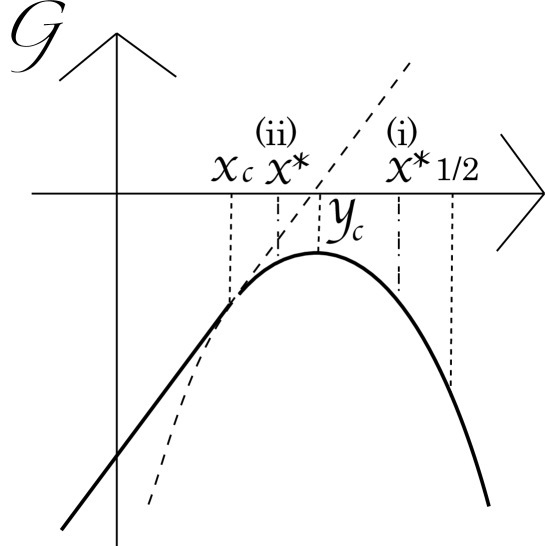
Figure 3: Schematic figure of ${\cal G}(y)$ for $\beta>\beta_{c}$ and $\alpha>1$. The maximum value in the integration range $y<x^{*}$ determines the asymptotic behavior $\phi(n)=\lim_{N\to\infty}N^{-1}\log\left\langle Z^{n}\right\rangle$.

1. $y_{c}<x^{*}$
   As $y_{c}$ and $x^{*}$ are parameterized as $y_{c}=e^{-n\beta}/(1+e^{-n\beta})$ and $x^{*}=e^{-\beta_{c}}/(1+e^{-\beta_{c}})$, respectively, this holds for $n>n_{c}\equiv\beta_{c}/\beta$. In this case, ${\cal G}(y)$ is maximized at $y=y_{c}$, as shown in figure 3, which means eq. (45) can be assessed as $\left\langle Z^{n}\right\rangle\sim\exp\left[N\left({\cal G}(y_{c})+n\alpha\beta/2\right)\right]$. This yields the thermodynamic limit

   $$\phi(n)=\lim_{N\rightarrow\infty}\frac{1}{N}\log{\left\langle Z^{n}\right\rangle}=\log{2}+\alpha\log\left(\cosh\left(\frac{n\beta}{2}\right)\right),$$ (47)

   which coincides with $\phi_{\rm RS2}(n)$.

2. $y_{c}>x^{*}$
   This holds for $n<n_{c}$. Figure 3 indicates that ${\cal G}(y)$ is maximized at $y=x^{*}$, which is the right-end point of the integration range. In this case, the asymptotic behavior is given as

   $$\phi(n)=\lim_{N\rightarrow\infty}\frac{1}{N}\log{\left\langle Z^{n}\right\rangle}=n\alpha\beta\left(\frac{1}{2}-x^{*}\right)=\frac{n\alpha\beta}{2}\tanh{\frac{\beta_{c}}{2}}.$$ (48)

   This is identical to $\phi_{\rm 1RSB}(n)$.

The analyticity breaking at $n=n_{c}$ for $\phi(n)=\lim_{N\to\infty}\phi_{N}(n)=\lim_{N\to\infty}N^{-1}\log\left\langle Z^{n}\right\rangle$ can be interpreted as follows [14, 10]. In the low temperature phase of $\beta>\beta_{c}$, it is considered that REM of each sample is dominated by a few states of minimum energy. This means that the free energy density in this phase can be roughly expressed as $-(N\beta)^{-1}\log Z\simeq N^{-1}\epsilon_{\rm min}$, where $\epsilon_{\rm min}$ denotes the minimum value of the $2^{N}$ energy states $\epsilon_{1},\epsilon_{2},\ldots,\epsilon_{2^{N}}$. The theory of extreme value statistics [15] indicates that $y=M^{-1}\epsilon_{\rm min}+1/2$, obeys a Gumbel-type distribution, $P(y)$, which in the current system is characterized as

$$\frac{1}{N}\log P(y)=\left\{\begin{array}[]{ll}-\infty,&y>x^{*},\cr(1-\alpha)\log{2}+\alpha h(y),&0<y<x^{*},\end{array}\right.$$ (51)

as $N$ tends to infinity, where $x^{*}=h_{2}^{-1}(1-\alpha^{-1})$ represents the typical value of $y$. The physical implication of this behavior is that it is very rare for $y$ to fluctuate in the right direction because $y$ is given by the minimum of exponentially many energy values, while the fluctuation in the left direction obeys normal-type large deviation statistics described by a finite rate function. Eq. (51) indicates that if $y_{c}<x^{*}$ holds, which is the case for $n>n_{c}$, then $y=y_{c}=e^{-n\beta}/(1+e^{-n\beta})$, which corresponds to a rare low minimum energy, dominates $\left\langle Z^{n}\right\rangle=N\alpha\beta\omega^{-\frac{nM}{2}}\int dye^{-Nn\alpha\beta y}P(y)$, yielding $\phi(n)=\phi_{\rm RS2}(n)$. On the other hand, for $n<n_{c}$, $\left\langle Z^{n}\right\rangle$ is dominated by $y=x^{*}$, which corresponds to the typical value of the minimum energy, and the thermodynamic limit is provided as $\phi(n)=\phi_{\rm 1RSB}(n)$. These indicate that the origin of the 1RSB solution is a singularity of the distribution of the minimum energy, which arises in the thermodynamic limit and is characterized as eq. (51). The formula (17) makes it possible to more precisely describe the analyticity breaking of $\phi(n)$ brought about by this singularity.

4.2 Numerical assessment of the moment

The utility of eq. (17) is not limited to analysis in the thermodynamic limit; this formula is also useful for the numerical assessment of the moment for systems of finite size.

A representative approach to evaluate $\left\langle Z^{n}\right\rangle$ is to numerically average $Z^{n}$ by sampling $n_{0},n_{1},\ldots,n_{M}$ from eq. (10). This can be efficiently performed as follows (also shown in Appendix C of ref. [10]).

To generate $n_{0},n_{1},\ldots,n_{M}$ following eq. (10), we first sample $n_{0}$ from a binomial distribution

$$P(n_{0})=\frac{2^{N}!}{\left(2^{N}-n_{0}\right)!n_{0}!}p_{0}^{n_{0}}\left(1-p_{0}\right)^{2^{N}-n_{0}},$$ (52)

where $p_{0}=P(E_{0})$. For a generated $n_{0}$, we next sample $n_{1}$ from a conditional binomial distribution

$$P(n_{1}|n_{0})=\frac{\left(2^{N}-n_{0}\right)!}{\left(2^{N}-n_{0}-n_{1}\right)!n_{1}!}p_{1}^{n_{1}}\left(1-p_{1}\right)^{2^{N}-n_{0}-n_{1}},$$ (53)

where $p_{1}=P(E_{1})/(1-P(E_{0}))$. We repeat this process up to $n_{M-1}$; namely, for a generated set of $n_{0},n_{1},\ldots,n_{i-1}$, $n_{i}$ is sampled from a conditional binomial distribution

$$P(n_{i}|n_{0},n_{1},\ldots,n_{i-1})=\frac{\left(2^{N}-\sum_{k=0}^{i-1}n_{k}\right)!}{\left(2^{N}-\sum_{k=0}^{i}n_{k}\right)!n_{i}!}p_{i}^{n_{i}}\left(1-p_{i}\right)^{2^{N}-\sum_{k=0}^{i-1}n_{k}},$$ (54)

where $p_{i}=P(E_{i})/(1-\sum_{k=0}^{i-1}P(E_{k}))$. After generating $n_{0},n_{1},\ldots,n_{M-1}$ in this manner, $n_{M}$ is given as $n_{M}=2^{N}-\sum_{i=0}^{M-1}n_{i}$, which guarantees satisfaction of the strict constraint $\sum_{i=0}^{M}n_{i}=2^{N}$.

Since each step can be performed by an $O(1)$ computation, the necessary computational cost for this generation is $O(N)$ per sample, which is feasible. However, a problem remains in the evaluation of $\left\langle Z^{n}\right\rangle$ by this approach based on naive sampling.

The analysis shown in the preceding subsection indicates that in the low temperature phase $\beta>\beta_{c}$, $\left\langle Z^{n}\right\rangle$ of $n>n_{c}$ is dominated by samples of a rare low minimum energy value in the limit $N\to\infty$. This implies that accurate assessment of such moments requires an exponentially large number of samples since the probability of generating the dominant samples decreases exponentially with respect to $N$. On the other hand, the analysis also means that eq. (17) can be accurately evaluated by numerical integration. This is because the integrand of eq. (29) is practically localized in a finite interval due to the properties of large deviation statistics and therefore truncating the integration range to a finite interval yields little numerical error.

Figure 4 shows a comparison of the numerical evaluation of $\left\langle Z^{n}\right\rangle$ between the sampling and numerical integration approaches for the low temperature phase of $\alpha=2,\beta=3\beta_{c}$. In both approaches the system size was set to $N=10$ while the number of samples was varied as ${\cal N}_{\rm samples}=10,10^{3}$ and $10^{6}$. The figure shows that as $n$ increases, more samples are necessary to accurately evaluate $\left\langle Z^{n}\right\rangle$. This is consistent with the analysis in the preceding subsection indicating that $\left\langle Z^{n}\right\rangle$ for $n\raisebox{-2.15277pt}{$\>\stackrel{{\scriptstyle\textstyle>}}{{\sim}}\>$}n_{c}$ is dominated by samples of a rare low minimum energy. In the sampling approach, ${\cal N}_{\rm samples}=10^{6}$ achieves an accuracy similar to that of the numerical integration. However, more samples are necessary as $N$ increases because the probability of generating samples that dominate $\left\langle Z^{n}\right\rangle$ decreases exponentially with $N$. On the other hand, the necessary computational cost for evaluating $\left\langle Z^{n}\right\rangle$ is not greatly dependent on $N$ in the numerical integration, demonstrating a point of superiority of eq. (17).

Notice that eq. (17) holds not only for $n\in\mathbb{R}$ but also for $n\in\mathbb{C}$. This can be used for characterizing the breaking of the analyticity of $\left\langle Z^{n}\right\rangle$ by the convergence of the zeros of $\left\langle Z^{n}\right\rangle$ to the real axis on the complex $n$ plane as $N$ tends to infinity, which is analogous to a description of phase transitions by Lee and Yang [16] and Fisher [17]. As far as the authors know, the complex zeros with respect to $n$ have little been examined except for a few examples [18, 19] although zeros of the complex temperature or external field for typical samples of REMs were studied in preceding literature [8, 20]. A detailed analysis along this direction will be reported in a subsequent paper [21].

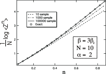
Figure 4: $\left\langle Z^{n}\right\rangle$ assessed by numerical integration of eq.(17) and a naive sampling scheme for $N=10$. The relevant parameters are $\alpha=2$ and $\beta=3\beta_{c}$, which corresponds to the low temperature phase.

5 Summary

In summary, we have developed an exact expression for the moment of the partition function of CDREM. The expression is valid not only in the thermodynamic limit but also for systems of finite size. This is useful for investigating the breaking of analyticity with respect to the replica number, which plays the role of the power of the moment, in the thermodynamic limit. Our approach demonstrates that the analyticity breaking due to a singularity in the distribution of the minimum energy is the origin of 1RSB observed in the low temperature phase of CDREM. We have also shown that the developed expression is useful for numerically evaluating the moment of finite size systems.

Although the uniqueness of analytical continuation from $n\in\mathbb{N}$ to $n\in\mathbb{C}$ is not guaranteed by Carlson’s theorem for generic REMs, the behavior predicted by our approach is qualitatively the same as that of CDREM. This implies that 1RSB observed in a wide class of REMs originates from the analyticity breaking with respect to the replica number $n$, which takes place in the thermodynamic limit $N\to\infty$ after analytical continuation from $n\in\mathbb{N}$ to $n\in\mathbb{C}$ is performed for finite $N$.

Appendix A Exact expression of $\left\langle Z^{n}\right\rangle$ for continuous random energy model

We here provide an exact expression of $\left\langle Z^{n}\right\rangle$ for the continuous random energy model, which was originally introduced by Derrida in [11]. In this model, $2^{N}$ states are distributed in energy $E$ with the following probability,

$$P(E)=\frac{1}{\sqrt{\pi NJ^{2}}}\exp{\left(-\frac{E^{2}}{NJ^{2}}\right)}.$$ (55)

The moment of the partition function $Z(\{E_{i}\})=\sum_{i=1}^{2^{N}}\exp{\left(-\beta E_{i}\right)}$ is expressed as

$$\left\langle Z^{n}\right\rangle=\int_{-\infty}^{\infty}\left(\prod_{i=1}^{2^{N}}dE_{i}P(E_{i})\right)Z^{n}\left(\{E_{i}\}\right).$$ (56)

Applying eq. (13) to $Z^{n}\left(\{E_{i}\}\right)$ yields

$$\left\langle Z^{n}\right\rangle = \frac{1}{\tilde{\Gamma}(-n)}\int_{H}d\rho(-\rho)^{-n-1}\prod_{i=1}^{2^{N}}\left(\int_{-\infty}^{\infty}dE_{i}P(E_{i})e^{-\rho\exp{\left(-\beta{E_{i}}\right)}}\right)$$ (57)

$$= \frac{1}{\tilde{\Gamma}(-n)}\int_{H}d\rho(-\rho)^{-n-1}\left(\int_{-\infty}^{\infty}dEP(E)e^{-\rho\exp{\left(-\beta{E}\right)}}\right)^{2^{N}}$$ (58)

$$= \frac{1}{\tilde{\Gamma}(-n)}\int_{H}d\rho(-\rho)^{-n-1}\left(\int_{-\infty}^{\infty}\frac{dE}{\sqrt{\pi NJ^{2}}}e^{-\frac{E^{2}}{NJ^{2}}-\rho\exp{\left(-\beta{E}\right)}}\right)^{2^{N}}.$$ (59)

Numerically evaluating this is computationally feasible for $\forall{N}$.

Deforming the contour $H$ to $\widetilde{H}:\infty+{\rm i}\epsilon\to+{\rm i}\epsilon\to-{\rm i}\epsilon\to\infty-{\rm i}\epsilon$ with an infinitesimal number $\epsilon$ (putting $\rho=re^{i(\theta-\pi)},\ \theta=-\pi,\pi$), in conjunction with $p>{\rm Re}(n)$ times employment of the integration by parts for removing the singularity at $\rho=0$, yields

$$\left\langle Z^{n}\right\rangle = \frac{1}{\Gamma(p-n)}\int_{0}^{\infty}dr\ r^{p-n-1}$$ (60)

$$\phantom{\frac{1}{\Gamma(p-n)}}\times\left(-\frac{\partial}{\partial r}\right)^{p}\left(\int_{-\infty}^{\infty}\frac{dE}{\sqrt{\pi NJ^{2}}}e^{-\frac{E^{2}}{NJ^{2}}-r\exp{\left(-\beta{E}\right)}}\right)^{2^{N}},$$ (61)

which is equivalent to eq. (7) of ref. [12].

From eq. (56), the behavior of the moment in the thermodynamic limit can be investigated in a manner similar to the analysis of CDREM. This investigation indicates that the moment behaves as

$$\phi(n)=\lim_{N\rightarrow\infty}\frac{1}{N}\log{\left\langle Z^{n}\right\rangle}=\left\{\begin{array}[]{ll}\log{2}+n^{2}\beta^{2}J^{2}/4,&n>n_{\rm RS},\cr n\left(\log{2}+{\beta^{2}J^{2}}/{4}\right),&n<n_{\rm RS},\end{array}\right.$$ (64)

for $\beta<\beta_{c}=2\sqrt{\log 2}/J$ in the thermodynamic limit, where $n_{\rm RS}=\beta_{c}^{2}/\beta^{2}>1$. On the other hand,

$$\phi(n)=\lim_{N\rightarrow\infty}\frac{1}{N}\log{\left\langle Z^{n}\right\rangle}=\left\{\begin{array}[]{ll}\log{2}+n^{2}\beta^{2}J^{2}/4,&n>n_{c},\cr{n\beta J\sqrt{\log{2}}},&n<n_{c},\end{array}\right.$$ (67)

holds for $\beta>\beta_{c}$, where $n_{c}=\beta_{c}/\beta<1$.

The inequality $Z\left(\{E_{i}\}\right)=\sum_{i=1}^{2^{N}}\exp\left(-\beta E_{i}\right)>\exp\left(-\beta E_{1}\right)$ gives

$$\left\langle Z^{n}\right\rangle^{1/N}>\left\langle e^{-n\beta E_{1}}\right\rangle^{1/N}=\exp\left(n^{2}\beta^{2}J^{2}/4\right),$$ (68)

for $n>0$, implying that $\left\langle Z^{n}\right\rangle^{1/N}$ is not upper-bounded by $e^{\pi|n|}$. This means that the uniqueness of the analytical continuation from $n\in\mathbb{N}$ to $n\in\mathbb{C}$ (${\rm Re}(n)\geq 0$) is not guaranteed by Carlson’s theorem for $\phi_{N}(n)=N^{-1}\log\left\langle Z^{n}\right\rangle$ in the continuous random energy model. However, RM successfully reproduces the behavior of eqs. (64) and (67). This implies that the transitions $\phi(n)=\lim_{N\to\infty}\phi_{N}(n)$ between the multiple solutions that arise in RM, including the 1RSB transition, are not due to multiple varieties of analytical continuation, but are brought about by the breaking of analyticity with respect to the replica number $n$ in a family of REMs.

Appendix B Replica analysis of CDREM

We here show how $\phi_{\rm RS1}(n)$, $\phi_{\rm RS2}(n)$ and $\phi_{\rm 1RSB}(n)$ are derived for CDREM by the replica method (RM). In order to evaluate $\left\langle Z^{n}\right\rangle$ for $n\in\mathbb{R}$ (or $n\in\mathbb{C}$), in RM the moment is first evaluated for $n\in\mathbb{N}$, for which the power series expansion can be used. This yields the expression

$$\left\langle Z^{n}\right\rangle = \left\langle\left(\sum_{A=1}^{2^{N}}e^{-\beta\epsilon_{A}}\right)^{n}\right\rangle=\sum_{A_{1},A_{2},\ldots,A_{n}}\left\langle e^{-\beta\sum_{a=1}^{n}\epsilon_{A_{a}}}\right\rangle$$ (69)

$$= \sum_{\left(p_{1},p_{2},\ldots,p_{n}\right)}{\cal W}\left(p_{1},p_{2},\ldots,p_{n}\right)\prod_{k=1}^{n}\left(I(k\beta)\right)^{p_{k}},$$ (70)

where

$$I(\beta)=\sum_{E}P(E)e^{-\beta E}\sim\exp\left[N\alpha\left(\log\left(\cosh\left(\frac{\beta}{2}\right)\right)\right)\right],$$ (71)

and ${\cal W}\left(p_{1},p_{2},\ldots,p_{n}\right)$ represents the number of ways of partitioning $n$ replicas $A_{1},A_{2},\ldots,A_{n}$ to $p_{1}$ states (out of $A=1,2,\ldots,2^{N}$) by one, to $p_{2}$ states by two, $\ldots$, and to $p_{n}$ states by $n$. Clearly, ${\cal W}\left(p_{1},p_{2},\ldots,p_{n}\right)=0$ unless $\sum_{k=1}^{n}kp_{k}=n$.

Eq. (71) indicates that each term in eq. (70) scales exponentially with respect to $N$ since ${\cal W}\left(p_{1},p_{2},\ldots,p_{n}\right)$ depends exponentially on $N$ as well. On the other hand, the number of varieties of partition $\left(p_{1},p_{2},\ldots,p_{n}\right)$ does not depend on $N$. This implies that the summation of eq. (70) is dominated by a single term labeled by a certain partition $\left(p_{1}^{*},p_{2}^{*},\ldots,p_{n}^{*}\right)$ and the exponent $\phi(n)=\lim_{N\to\infty}N^{-1}\log\left\langle Z^{n}\right\rangle$ can be accurately evaluated by only the single dominant term. Namely, $\left(p_{1},p_{2},\ldots,p_{n}\right)$ plays the role of a replica order parameter. It is noteworthy that this role is similar to that of the types in information theory. However, there is a distinct difference between the two notions because $\left(p_{1},p_{2},\ldots,p_{n}\right)$ represents relative positions of replicas in the replicated system while the types are defined for a single system.

The remaining problem is how to find the dominant partition. Replica symmetry, which implies that eq. (69) is invariant under any permutation of replica indices $a=1,2,\ldots,n$, offers a useful guideline for solving this problem. This leads to a physically natural assumption that the dominant partition is characterized by this symmetry as well, which yields the following two RS solutions:

• RS1: Dominated by $\left(p_{1}^{*},p_{2}^{*},\ldots,p_{n}^{*}\right)=(n,0,\ldots,0)$, giving

  $$\left\langle Z^{n}\right\rangle \sim 2^{Nn}\times\left(I(\beta)\right)^{n}$$ (72)

  $$\sim \exp\left[Nn\left(\log 2+\alpha\left(\log\left(\cosh\left(\frac{\beta}{2}\right)\right)\right)\right)\right].$$ (73)

  This gives $\lim_{N\to\infty}N^{-1}\log\left\langle Z^{n}\right\rangle=\phi_{\rm RS1}(n)$.

• RS2: Dominated by $\left(p_{1}^{*},p_{2}^{*},\ldots,p_{n}^{*}\right)=(0,0,\ldots,1)$, giving

  $$\left\langle Z^{n}\right\rangle \sim 2^{N}\times I(n\beta)$$ (74)

  $$\sim \exp\left[N\left(\log 2+\alpha\left(\log\left(\cosh\left(\frac{n\beta}{2}\right)\right)\right)\right)\right].$$ (75)

  This gives $\lim_{N\to\infty}N^{-1}\log\left\langle Z^{n}\right\rangle=\phi_{\rm RS2}(n)$.

Eqs. (73) and (75) indicate that $\phi_{\rm RS1}(n)$ and $\phi_{\rm RS2}(n)$ can be analytically continued from $n\in\mathbb{N}$ to $n\in\mathbb{R}$ (or $n\in\mathbb{C}$), respectively. The above equations also mean that $\phi_{\rm RS1}(n)$ and $\phi_{\rm RS2}(n)$ agree at $n=1$ in general, which makes it difficult to choose the relevant solution for $n<1$. As a practical solution, we select, as the relevant solution in this region, the solution with the larger first derivative, following an empirical criterion given in ref. [10]. This gives $\phi(n)=\phi_{\rm RS1}(n)$ for $\beta<\beta_{c}$, while $\phi(n)=\phi_{\rm RS2}(n)$ is chosen for $\beta>\beta_{c}$. However, in the latter case, $\phi_{\rm RS2}(n)$ is inadequate for $n<n_{c}=\beta_{c}/\beta<1$ because the convexity condition $\left(\partial/\partial n\right)\left(n^{-1}\phi_{\rm RS2}(n)\right)\geq 0$ is not satisfied. Therefore, we have to construct another solution taking the breaking of replica symmetry into account, which yields the 1RSB solution:

• 1RSB: Dominated by $p_{m}^{*}=n/m$ for a certain $m$ and $p_{k}^{*}=0$ for $k\neq m$, giving

  $$\left\langle Z^{n}\right\rangle \sim 2^{Nn/m}\times\left(I(m\beta)\right)^{n/m}$$ (76)

  $$\sim \exp\left[N\frac{n}{m}\left(\log 2+\alpha\left(\log\left(\cosh\left(\frac{m\beta}{2}\right)\right)\right)\right)\right].$$ (77)

  After analytical continuation, $m$ is determined so as to extremize the right hand side, which leads to $m=n_{c}=\beta_{c}/\beta$. It may be noteworthy that the extremum means not maximum but minimum. This gives $\lim_{N\to\infty}N^{-1}\log\left\langle Z^{n}\right\rangle=\phi_{\rm 1RSB}(n)$.

Figure 2 schematically shows the profiles of the three solutions.

References

References

- [1] Mézard M, Parisi G and Virasoro M A 1987 Spin Glass Theory and Beyond (Singapore: World Scientific)
- [2] Dotzenko V S 2001 Introduction to the Replica Theory of Disordered Statistical Systems (Cambridge: Cambridge University Press)
- [3] Talagrand M 2003 Spin Glasses: A Challenge for Mathematicians. Mean Field Models and Cavity Method (Berlin: Springer Verlag)
- [4] Talagrand M 2006 Ann. Math. 163 221
- [5] Titchmarsh E C 1932 The Theory of Functions (Oxford: Oxford University Press)
- [6] Sherrington D and Kirkpatrick S 1975 Phys. Rev. Lett. 35 1972
- [7] van Hemmen J L and Palmer R G 1979 J. Phys. A: Math. Gen.12 563
- [8] Moukarzel C and Parga N 1991 Physica A177 24
- [9] Moukarzel C and Parga N 1992 Physica A185 305
- [10] Ogure K and Kabashima Y 2004 Prog. Theor. Phys. 111 661
- [11] Derrida B 1981 Phys. Rev. B 24 2613
- [12] Gardner E and Derrida B 1989 J. Phys. A: Math. Gen.22 1975
- [13] Csiszár I and Körner J 1982 Information Theory: Coding Theorems for Discrete Memoryless Systems (Orlando: Academic Press)
- [14] Bouchaud J-P and Mézard M 1997 J. Phys. A: Math. Gen.30 7997
- [15] Gumbel E J 1958 Statistics of Extremes (New York: Columbia University Press)
- [16] Lee L D and Yang C N 1952 Phys. Rev. 87 410
- [17] Fisher M E 1965 Lectures in Theoretical Physics vol. 7 (Boulder: University of Colorado Press)
- [18] Ogure K and Kabashima Y 2005 Prog. Theor. Phys. Suppl. 157 103
- [19] Obuchi Y, Kabashima Y and Nishimori H 2009 J. Phys. A: Math. Theor. 42 075004 (27pp)
- [20] Derrida B 1991 Physica A177 31
- [21] Ogure K and Kabashima Y On analyticity with respect to the replica number in random energy models II: zeros on the complex plane Preprint arXiv:0812.4655