Realistic analytic model for the prompt and high latitude emission in GRBs

Abstract

Most gamma-ray bursts (GRBs) observed by the Swift satellite show an early steep decay phase (SDP) in their X-ray lightcurve, which is usually a smooth continuation of the prompt gamma-ray emission, strongly suggesting that it is its tail. However, the mechanism behind it is still not clear. The most popular model for this SDP is High Latitude Emission (HLE), in which after the prompt emission from a (quasi-) spherical shell stops photons from increasingly large angles relative to the line of sight still reach the observer, with a smaller Doppler factor. This results in a simple relation between the temporal and spectral indexes, $\alpha=2+\beta$ where $F_{\nu}\propto t^{-\alpha}\nu^{-\beta}$. While HLE is expected in many models for the prompt GRB emission, such as the popular internal shocks model, there are models in which it is not expected, such as sporadic magnetic reconnection events. Therefore, testing whether the SDP is consistent with HLE can help distinguish between different prompt emission models. In order to adequately address this question in a careful quantitative manner we develop a realistic self-consistent model for the prompt emission and its HLE tail, which can be used for combined temporal and spectral fits to GRB data that would provide strict tests for the HLE model. We model the prompt emission as the sum of its individual pulses with their HLE tails, where each pulse arises from an ultra-relativistic uniform thin spherical shell that emits isotropically in its own rest frame over a finite range of radii. Analytic expressions for the observed flux density are obtained for the internal shock case with a Band function emission spectrum. We find that the observed instantaneous spectrum is also a Band function. Our model naturally produces, at least qualitatively, the observed spectral softening and steepening of the flux decay as the peak photon energy sweeps across the observed energy range. The observed flux during the SDP is initially dominated by the tail of the last pulse, but the tails of one or more earlier pulses can become dominant later on. A simple criterion is given for the dominant pulse at late times. The relation $\alpha=2+\beta$ holds also as $\beta$ and $\alpha$ change in time. Modeling several overlapping pulses as a single wider pulse would over-predict the emission tail.

1 Introduction

Before the launch of the Swift satellite (Gehrels et al. 2004), Gamma Ray burst (GRB) X-ray afterglows were detected at least several hours after the burst (Soffitta et al. 2004 and references therein). They typically displayed a power law decay $\sim t^{-1}-t^{-1.5}$ around their detection time (De Pasquale et al. 2006). Swift’s ability to rapidly and autonomously slew when the Burst Alert Telescope (BAT, observing in the energy range $15-350\;$keV; Barthelmy et al. 2005) instrument detects a GRB enables it to point its other instruments - the X-Ray Telescope (XRT, observing in the energy range $0.2-10\;$keV; Burrows et al. 2005a) and UV/Optical Telescope (UVOT, observing at wavelengths $170-650\;$nm, i.e. from the optical to the near UV; Roming et al. 2005) - toward the GRB within tens of seconds from the GRB trigger time.The XRT thus filled the observational gap between the end of the prompt emission and the beginning of the pre-Swift afterglow observations several hours later. It revealed a complex behaviour usually consisting of three phases, followed by most GRBs, and referred to as a canonical light curve (Nousek et al. 2006), consisting of three distinct power-law segments where $F_{\nu}\propto t^{-\alpha}$: an initial (at $t<t_{\rm break,1}$, with $300\;{\rm s}\lesssim t_{\rm break,1}\lesssim 500\;{\rm s}$) very steep decay with time $t$ (with a power-law index $3\lesssim\alpha_{1}\lesssim 5$; see also Bartherlmy et al. 2005; Tagliaferri et al. 2005); a subsequent (at $t_{\rm break,1}<t<t_{\rm break,2}$, with $10^{3}\;{\rm s}\lesssim t_{\rm break,2}\lesssim 10^{4}\;{\rm s}$) very shallow decay ($0.2\lesssim\alpha_{2}\lesssim 0.8$); and a final steepening (at $t>t_{\rm break,2}$) to the familiar pre-Swift power-law behaviour ($1\lesssim\alpha_{3}\lesssim 1.5$). In many cases there are X-ray flares superimposed on this underlying smooth component (typically during the first two phases, at $t<t_{\rm break,2}$; Burrows et al. 2005b; Falcone et al. 2006; Krimm et al. 2007), and in some cases there is a later (at $t_{j}>t_{\rm break,2}$) further steepening due to a jet.

The third decay phase ($F_{\nu}\propto t^{-\alpha_{3}}$) is the afterglow emission that was observed before Swift and is well explained by synchrotron radiation from the forward shock that is driven into the external medium as the GRB ejecta are decelerated, where the energy in the afterglow shock is constant in time (no significant energy gains or losses). The plateau (or shallow decay) phase can be explained either by pre-Swift models or by later models that have been developed especially for this purpose (Nousek et al. 2006; Panaitescu et al. 2006; Granot 2007). It could be due to energy injection, either by a tail of decreasing Lorentz factors at the end of the ejection phase (Rees & Mészaros 1998; Sari & Mészaros 2000; Ramirez-Ruiz, Merloni & Rees 2001; Granot & Kumar 2006) or by a relativistic wind produced by a long lasting source activity (Rees & Mészaros 2000; McFadyen et al. 2001; Lee & Ramirez-Ruiz 2002; Dai 2004; Ramirez-Ruiz 2004), by an increasing efficiency of X-ray afterglow emission due to time dependence of the shock microphysics parameters (Granot, Königl & Piran 2006), by a viewing angle slightly outside the region of prominent afterglow emission (Eichler & Granot 2006), by a contribution from the reverse-shock (Genet, Daigne & Mochkovitch 2007) or by a two component jet model (Peng, Königl & Granot 2005; Granot, Königl & Piran 2006).

The steep decay phase is observed in most bursts, and is in the great majority of cases a smooth continuation of the prompt emission, both temporally and spectrally (O’Brien et al. 2006). This strongly suggests that it is the tail of the prompt emission. Several explanations for this phase have been suggested in the context of previously existing models (Tagliaferri et al. 2005; Nousek et al. 2006), such as emission from the hot cocoon in the collapsar model (Mészaros & Rees 2001, Ramirez-Ruiz et al. 2002). The most popular model, by far, is High Latitude Emission (HLE) originally referred to as emission from a “naked” GRB (Kumar and Panaitescu 2000a). In this model the prompt GRB emission is from a (quasi-) spherical shell, and after it turns off at some radius then photons keep reaching the observer from increasingly larger angles relative to the line of sight, due to the the added path length caused by the curvature of the emitting region. Such late arriving photons experience a smaller Doppler factor. This leads to a simple relation between the temporal and spectral indexes, $\alpha=2+\beta$ where $F_{\nu}(t)\propto t^{-\alpha}\nu^{-\beta}$, that holds at late times when $t-t_{0}\gg\Delta t$, where $t_{0}$ and $\Delta t$ are the start time and width of the pulse, respectively. The steep decay phase also shows a softening of the spectrum with time (see Zhang et al. 2007 and references therein).

The consistency of the steep decay phase with HLE has been studied by several authors (Nousek et al. 2006; Liang et al. 2006; Butler & Kocevski 2007; Zhang et al. 2007; Qin 2008). However, some simplifying assumptions were usually made, which may affect the comparison between this model and the observations. One such assumption is the choice of the reference time $t_{0}$ for the steep decay, especially when the prompt emission consists of several pulses. Liang et al. (2006) find that when assuming the HLE relation $\alpha=2+\beta$ and fitting for $t_{0}$ its derived value is consistent with the onset of the last pulse of the prompt emission (or of the individual spike or flare whose tail is being fit). Zhang et al. (2007) find that the HLE cannot explain the steep decays accompanied by a spectral softening, but can explain the cases with no observed spectral evolution. Barniol Duran and Kumar (2008) find that only $20\%$ of their sample is consistent with HLE. Butler & Kocevski (2007) find that for a (physically motivated) time independent soft X-ray absorption (fixed N_H) the spectrum during the steep decay phase, is much better fit by an intrinsic Band function spectrum (Band et al. 1993) rather than by a power-law, and that the peak photon energy shifts to lower energies with time. Qin (2008) finds that such a behavior can, at least qualitatively, be produced for a delta function emission in radius with a Band function spectrum. It is therefore still a largely open question whether the temporal and spectral properties of the steep decay are consistent with HLE. Moreover, it appear that a physically motivated model for the prompt emission with realistic assumptions about the emission (e.g. over a finite range of radii with a Band function emissivity) is needed in order to address this question in a more quantitative and fully self consistent manner.

The nature of the prompt GRB emission is what ultimately determines the properties of its tail. HLE is expected only in models where the prompt emission is from a quasi-spherical shell and turns off rather abruptly at some finite radius (or lab frame time). The best example for this type of model is internal shocks (Rees & Mészaros 1994; Sari & Piran 1997) where variability in the Lorentz factor of the relativistic GRB outflow causes faster shells of ejecta to collide with slower sells resulting in shocks going into the shell over a finite range of radii (typically $\Delta R\sim R$). On the other hands, there are models in which HLE is not expected, such as in the case of isolated sporadic magnetic reconnection events within a Poynting flux dominated outflow (e.g. Lyutikov & Blandford 2003) in which each spike in the GRB light curve is from a distinct small and well localized region. Therefore, testing whether the steep decay phase is consistent with HLE would help distinguish between these two types (or classes) of prompt GRB models. This can be an important step toward identifying the basic underlying mechanism for the prompt emission, which is still one the the most striking open questions in GRB research more than four decades after the discovery of GRBs.

In order to address this question, we develop a model for the prompt and its HLE tail that is physically motivated, realistic, and easy to use (fully analytic in its simplest version) in global joint fits (to all of the available data at all times and photon energies) of the prompt GRB and its SDP tail. Such global fits can provide a stringent and fully self-consistent test of HLE model for the SDP in GRBs.

The prompt emission is modeled as the sum of a finite number of pulses. Each pulse corresponds to a spike in the prompt GRB light curve and has its own HLE tail. An individual spike is modeled as arising from a thin uniform spherical relativistic shell that emits isotropically in its own rest frame over a finite range of radii, while the observed flux is calculated by integrating over the equal arrival time surface (Granot, Piran & Sari 1999; Granot 2005; Granot, Cohen-Tanugi & do Couto e Silva 2008) of photons to a distant observer. Our model is particularly suitable for internal shocks, which we focus on in this paper. For the emitted spectrum we consider the phenomenological Band function, which provides a good fit the the prompt emission spectrum of the vast majority of GRBs. We point out that our model can also be used for X-ray flares, which appear to have temporal and spectral properties similar to the spikes of the prompt GRB emission. The main text provides the most useful results in an easy to use form, while the full derivations of these results are provided in appendixes in order to help understand their origin and make it easier to extend or generalize our model. We stress here that our main aim is not necessarily to uniquely determine all of the model parameters, which may be subject to various degeneracies and may prove hard when fitting to real data, but instead to test whether our model can provide a good fit to the data for any set of physical parameters. While such a good fit would still not prove that the HLE must be at work, it would definitely support HLE as a viable and arguably most plausible model. Our model for an individual pulse is described in § 2, and results for the flux in the case for internal shocks with a Band function spectrum are given in § 3. The dependence of a single pulse on the model parameters is then investigated in § 4, while § 5 discusses how to combine several pulses in order obtain to the total prompt emission and its tail. Both are intended to help the reader when using our model to fit data, which is one of the main aims of our paper. Our conclusions are discussed in § 6. This paper describes in detail our theoretical model and its main properties, and stresses some important caveats that one should keep in mind when using it to fit data in order to test the HLE model. In subsequent work we intend to confront it with Swift BAT+XRT data.

2 Description of the Model

2.1 The Basic Physical Model

We consider an ultra-relativistic ($\Gamma\gg 1$) thin (of width $\ll R/\Gamma^{2}$) spherical expanding shell that emits over a range of radii $R_{0}\leqslant R\leqslant R_{f}\equiv R_{0}+\Delta R$. The emission turns on at radius $R_{0}$ and turns off at radius $R_{f}\geq R_{0}$. The Lorentz factor of the emitting shell is assumed to scale as a power-law with radius, $\Gamma^{2}=\Gamma_{0}^{2}(R/R_{0})^{-m}$ where $\Gamma_{0}\equiv\Gamma(R_{0})$. The emission is assumed to be isotropic in the comoving frame of the shell, and uniform over the shell, i.e. the comoving spectral luminosity depends only on the radius of the shell, $L^{\prime}_{\nu^{\prime}}=L^{\prime}_{\nu^{\prime}}(R)$. As the main purpose of this work is to check the consistency of the tail of the prompt emission with HLE, we need to model the prompt emission. We therefore use for the emission spectrum the phenomenological Band function (Band et al. 1993) spectrum that provides a good fit to the observed prompt emission spectrum of the vast majority of GRBs. In the following we mainly consider emission over a finite range of radii, $R_{0}\leq R\leq R_{f}=R_{0}+\Delta R$. The comoving luminosity is then:

$$L^{\prime}_{\nu^{\prime}}=L^{\prime}_{0}\left(\frac{R}{R_{0}}\right)^{a}S\left(\frac{\nu^{\prime}}{\nu^{\prime}_{p}}\right)\ ,\qquad\qquad S(x)=e^{1+b_{1}}\left\{\begin{array}[]{ll}x^{b_{1}}e^{-(1+b_{1})x}&x\leqslant x_{b}\ ,\\ x^{b_{2}}x_{b}^{b_{1}-b_{2}}e^{-(b_{1}-b_{2})}&x\geqslant x_{b}\ ,\end{array}\right.$$ (3)

where $\nu^{\prime}_{p}(R)\equiv\nu^{\prime}_{0}(R/R_{0})^{d}$ is the frequency where $\nu^{\prime}L^{\prime}_{\nu^{\prime}}(R)$ peaks, with $\nu^{\prime}_{0}\equiv\nu^{\prime}_{p}(R_{0})$; $x_{b}=(b_{1}-b_{2})/(1+b_{1})$, while $b_{1}$ and $b_{2}$ are the high and low energy slopes of the spectrum. For $b_{1}>-1>b_{2}$ the Band function has a peak in the $\nu F_{\nu}$ spectrum, at $x=1$, and therefore since $S(x)$ is normalized such that $S(x)=xS(x)=1$ at $x=1$, it will not affect normalization of $\nu F_{\nu}$ at its peak. The two functional forms used in the band function are matched at $\nu^{\prime}_{b}=x_{b}\nu^{\prime}_{p}$. The peak luminosity $L^{\prime}_{\nu^{\prime}_{p}}$ evolve as a power-law with radius, $L^{\prime}_{\nu^{\prime}_{p}}=L^{\prime}_{0}(R/R_{0})^{a}$ where $L^{\prime}_{0}=L^{\prime}_{\nu^{\prime}_{p}}(R_{0})$ is a normalization factor.

Throughout the paper, primed quantities are quantities measured in the comoving frame (i.e. the local rest frame of the emitting shell), unprimed quantities are measured either in the source rest frame (the lab frame, i.e. the cosmological frame of the GRB; this includes $\Gamma$, $R$, $\theta$ and $t$) or the observer frame (this refers to observed quantities, such as $F_{\nu}$, $\nu$ and $T$).

2.2 Calculating the Observed Flux

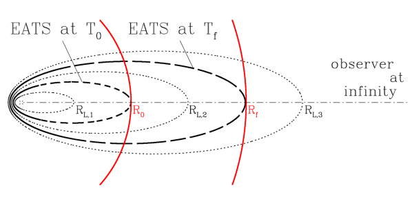
Figure 1: Illustration of Equal Arrival Time Surfaces (EATS). The particular EATS shown here are for a coasting shell ($m=0$), and are ellipsoids (Rees 1966) with an ellipticity $\epsilon=\beta$ and a semi-major to semi-minor axis ration of $\Gamma$ (which for display purposes is only 3 here). The red solid lines correspond to the inner ($R_{0}$) and outer ($R_{f}$) radii of the emission region. We call $R_{L}(T)$ the outermost radius of the EATS at observed time $T$. Shown are the EATS for the limiting cases corresponding to $R_{L}=R_{0}$ ($T=T_{\rm ej}+T_{0}$; thick short-dashed line) and $R_{L}=R_{f}$ ($T=T_{\rm ej}+T_{f}$; thick long-dashed line) as well as representative cases for $R_{L}<R_{0}$, $R_{0}<R_{L}<R_{f}$ and $R_{L}>R_{f}$ (dotted lines). For $R_{L}<R_{0}$ the EATS does not intersect the emission region, and therefore the first photons start reaching the observer only at $T=T_{\rm ej}+T_{0}$ from $R=R_{0}$ along the line of sight. At $R_{0}<R_{L}<R_{f}$ the flux typically rises (for $\Delta R\lesssim R_{0}$). At $T=T_{\rm ej}+T_{f}$ the last photons from the line of sight (at $R=R_{f}$) reach the observer, while for $T>T_{\rm ej}+T_{f}$ the front part of the EATS, which would otherwise contribute the most to the observed flux, sticks outside of the emission radius resulting in a sharp decay in the observed flux, which is then dominated by emission from large angles relative to the line of sight (HLE).

The observer is assumed to be located at a distance from the source that is much larger than the source size, so that the angle extended by the source as seen by the observer is very small and the observer effectively at “infinity”. In order to calculate the flux density $F_{\nu}$ that reaches the observer at an observed time $T$ we integrate the luminosity $L^{\prime}_{\nu^{\prime}}$ over the Equal Arrival Time Surface (EATS; see Figure 1), i.e. the locus of points from which photons that are emitted by the shell at a radius $R$, angle $\theta$ relative to the line of sight, and a lab frame time $t$, reach the observer simultaneously at an observed time $T$ (for full derivation see Appendix A).

2.3 Expected parameters values for internal shocks

The internal shocks model is the most popular model for the prompt GRB emission. Moreover, our model is very suitable for internal shocks. Therefore, we consider it in the following. Here we calculate the scalings of the various quantities with radius, that are expected for the internal shocks model. First, when different shells (i.e. parts of the outflow with different Lorentz factors) collide, they are expected to be in the coasting phase, corresponding to $m=0$. Moreover, for the simplest case of uniform shells, the strength of the shocks going into the two shells, as characterized by the relative upstream to downstream Lorentz factor, $\Gamma_{ud}$, is expected to be roughly constant with radius while the shock are crossing the shells. The electrons are expected to be fast cooling, i.e. cool significantly on a timescale much shorter than the shell crossing time of the shock, and therefore most of the emission is expected to arise from a thin cooling layer behind the shock. Therefore our thin shell approximation is expected to be reasonably valid. Admittedly, we use one emitting thin shell, corresponding to a single shock front, while the shock going into the other shell is not explicitly modeled. One could always model such a second shock by adding another thin emitting shell that turns on and off at the same radii ($R_{0}$ and $R_{f}$, respectively) but has a slightly smaller or larger Lorentz factor. This will not introduce a big difference in the overall result, so for the sake of simplicity we do not include this here.

Now we turn to find the expected scaling of $L^{\prime}_{\nu^{\prime}_{p}}$ and $\nu^{\prime}_{p}$ with radius, under the assumption that the observed soft gamma-ray range is dominated by synchrotron emission. For fast cooling, the peak frequency $\nu^{\prime}_{p}$ of the $\nu F_{\nu}$ spectrum is $\nu^{\prime}_{m}\approx(eB^{\prime}\gamma_{m}^{2})/(2\pi m_{e}c^{2})$ where $dN_{e}/d\gamma_{e}\propto\gamma_{e}^{-p}$ for $\gamma_{e}>\gamma_{m}$ where $\gamma_{m}=(p-2)/(p-1)(\epsilon_{e}/\xi_{e})(m_{p}/m_{e})(\Gamma_{ud}-1)$, while $\epsilon_{e}$ is the fraction of the internal energy behind the shock in the power law distribution of the relativistic electron, and $\xi_{e}$ is the fraction of all electrons taking part in this power energy distribution (and an electron-proton plasma is assumed for the composition of the outflow). As mentioned above, $\Gamma_{ud}$ is expected to be roughly constant during the shell crossing (for roughly uniform colliding shells), and therefore $\gamma_{m}$ would also be approximately constant, so that $\nu^{\prime}_{p}\propto B^{\prime}$. The magnetic field is expected to be predominantly normal to the radial direction, so that $B^{\prime}\approx B/\Gamma\propto B$ for $m=0$. Moreover, $B\propto R^{-1}$ is expected both for a magnetic field convected from the central source, and for a field generated at the shock that hold some constant fraction ($\epsilon_{B}$) of the internal energy behind the shock. Therefore, one expects the peak frequency to evolve as $\nu^{\prime}_{p}\propto R^{-1}$. We have also assumed $L^{\prime}_{\nu^{\prime}_{p}}\propto(R/R_{0})^{a}$. For synchrotron emission $L^{\prime}_{\nu^{\prime},{\rm max}}\propto N_{e}B^{\prime}\propto R^{0}$ as the number of emitting electron is proportional to the radius, $N_{e}\propto R$. Since the cooling break frequency scales as $\nu^{\prime}_{c}\propto R$, we have $L^{\prime}_{\nu^{\prime}_{p}}\approx L^{\prime}_{\nu^{\prime},{\rm max}}(\nu^{\prime}_{m}/\nu^{\prime}_{c})^{-1/2}\propto R^{1}$, implying $a=1$.

More generally (without specifying the emission mechanism) for roughly uniform shells with constant $\Gamma_{ud}$ both the rate at which particles cross the shock and the average energy per particle are constant with radius, implying a constant rate of internal energy generation ($dE^{\prime}_{\rm int}/dt^{\prime}\propto R^{0}$), and therefore for fast cooling this also applies for the total comoving luminosity, $L^{\prime}\sim\nu^{\prime}_{p}L^{\prime}_{\nu^{\prime}_{p}}\propto R^{0}$, and therefore $d+a=0$. This is indeed satisfied for synchrotron emission for which $d=-1$ and $a=1$, and holds more generally for other emission mechanisms in the fast cooling regime.

For now on the values $m=0$ and $d=-1$ derived in this part will be used throughout the paper. However, since the expressions do not become much simpler by specifying the value of $a$, we leave $a$ in the simpler expressions, and use the value of $a=1$ for figures only. In particular, all the figures showing lightcurves in this paper use these parameter values, as well as the mean BATSE values for the Band function spectral slopes: $b_{1}=-0.25$ and $b_{2}=-1.25$ (Preece et al., 2000).

2.4 Relevant Times and Timescales

A photon emitted from the source (at the origin) when the shell is ejected from it (i.e. at a lab frame time $t_{\rm ej}$ when the shell radius is $R=0$) arrives at the observer at an observer time $T_{\rm ej}$ which can be thought of as the observed ejection time of the shell. We define $T_{0}$ the initial radial time by $T=T_{\rm ej}+T_{0}$ being the time at which the first photons emitted reach the observer (that is, photons emitted at a radius $R_{0}$ along the line of sight). We also define $T_{f}$ the final angular time by $T=T_{\rm ej}+T_{f}$ being the time at which the last photons that are emitted along the line of sight (from $R_{f}$ and $\theta=0$) reach the observer.

For a constant Lorentz factor with radius ($m=0$), as expected for internal shocks, the expressions for $T_{0}$ and $T_{f}$ are simple:

$$T_{0}=\frac{(1+z)R_{0}}{2c\Gamma_{0}^{2}}\ ,\qquad\qquad T_{f}=T_{0}\left(1+\frac{\Delta R}{R_{0}}\right)\ .$$ (4)

We also define two normalized times (and their corresponding values at $T_{f}$) that will be used in the following:

$$\tilde{T}\equiv 1+\bar{T}\equiv\frac{T-T_{\rm ej}}{T_{0}}\ ,\qquad\qquad\tilde{T}_{f}\equiv 1+\bar{T}_{f}\equiv\frac{T_{f}}{T_{0}}=1+\frac{\Delta R}{R_{0}}\ ,$$ (5)

where $\tilde{T}=1$ (or $\bar{T}=0$) corresponds to the onset of the spike – the very first photon that reaches the observer (emitted at $R_{0}$ on the line of sight). The main motivation for defining these two times is that they correspond to the two most natural choices for the zero to, $\tilde{T}=0$ corresponding to the ejection time of the shell, and $\bar{T}=0$ corresponding to the onset of the spike in the lightcurve. The choice of the zero time is important for the definition of the temporal index in § 4.1, where we explore these two choices in detail. Moreover, it is more convenient to use $\bar{T}$ in some expressions and $\tilde{T}$ in others.

3 Results for Internal shocks with a Band function spectrum

3.1 Emission from a single radius

Before to turn to the more generic case of emission from a range of radii, we first consider the limiting case of emission from a single radius $R_{0}$. The peak frequency is then $\nu^{\prime}_{p}=\nu^{\prime}_{0}$, and the luminosity is

$$L^{\prime}_{\nu^{\prime}}=L^{\prime}_{0}S\left(\frac{\nu^{\prime}}{\nu^{\prime}_{p}}\right)R_{0}\delta(R-R_{0})\ ,$$ (6)

which after some algebra (see appendix A for details, and in particular section A.3) we obtain the flux:

$$F_{\nu}(\tilde{T}\geq 1)=\frac{(1+z)}{4\pi d_{L}^{2}}L_{0}\tilde{T}^{-2}S\left(\frac{\nu}{\nu_{0}}\tilde{T}\right)\ ,$$ (7)

where $d_{L}$ and $z$ are the luminosity distance and cosmological redshift of the source, $L_{0}\equiv 2\Gamma_{0}L^{\prime}_{0}$ and $\nu_{0}\equiv 2\Gamma_{0}\nu^{\prime}_{0}/(1+z)$. Denoting $F_{s}\equiv L_{0}(1+z)/(4\pi d_{L}^{2})$ and using the explicit expression for the Band function (eq. [3]), the observed flux reads

$$\frac{F_{\nu}(\tilde{T}\geq 1)}{F_{s}} = \left\{\begin{array}[]{ll}\tilde{T}^{b_{1}-2}(\nu/\nu_{0})^{b_{1}}e^{(1+b_{1})[1-\tilde{T}\nu/\nu_{0}]}&\tilde{T}\leqslant x_{b}\nu_{0}/\nu\ ,\\ \\ \tilde{T}^{b_{2}-2}(\nu/\nu_{0})^{b_{2}}x_{b}^{b_{1}-b_{2}}e^{1+b_{2}}&\tilde{T}\geqslant x_{b}\nu_{0}/\nu\ .\end{array}\right.$$ (11)

3.2 Emission from a finite range of radii

Integrating the luminosity (eq. (3)) over the Equal Arrival Time Surface (for details of the calculation see appendix A, and in particular its section A.4) leads to the following expression for the flux:

$$F_{\nu}(\tilde{T}\geq 1)=F_{0}\tilde{T}^{-2}\left[\min\left(\tilde{T},\tilde{T}_{f}\right)^{2+a}-1\right]S\left(\frac{\nu}{\nu_{0}}\tilde{T}\right)\ ,$$ (12)

where $F_{0}\equiv(1+z)L_{0}/[(2+a)4\pi d_{L}^{2}]$. This can be explicited as:

$$\frac{F_{\nu}(\tilde{T}\geq 1)}{F_{0}}=\left\{\begin{array}[]{ll}(\nu/\nu_{0})^{b_{1}}\tilde{T}^{b_{1}-2}\left(\tilde{T}^{2+a}-1\right)e^{(1+b_{1})(1-\tilde{T}\,\nu/\nu_{0})}&\tilde{T}<\min\left[\tilde{T}_{f},x_{b}\nu_{0}/\nu\right]\ ,\\ \\ (\nu/\nu_{0})^{b_{1}}\tilde{T}^{b_{1}-2}\left[\tilde{T}_{f}^{2+a}-1\right]e^{(1+b_{1})(1-\tilde{T}\,\nu/\nu_{0})}&\tilde{T}_{f}<\tilde{T}<x_{b}\nu_{0}/\nu\ ,\\ \\ (\nu/\nu_{0})^{b_{2}}\tilde{T}^{b_{2}-2}\left(\tilde{T}^{2+a}-1\right)x_{b}^{b_{1}-b_{2}}e^{1+b_{2}}&x_{b}\nu_{0}/\nu<\tilde{T}<\tilde{T}_{f}\ ,\\ \\ (\nu/\nu_{0})^{b_{2}}\tilde{T}^{b_{2}-2}\left[\tilde{T}_{f}^{2+a}-1\right]x_{b}^{b_{1}-b_{2}}e^{1+b_{2}}&\tilde{T}>\max\left[\tilde{T}_{f},x_{b}\nu_{0}/\nu\right]\ .\end{array}\right.$$ (13)

Note that the observed function has exactly the same shape as the local spectral emissivity – a pure Band function. This occurs only for $m=0$ and $d=-1$.

In terms of number of photons $N$ per unit photon energy $E$, area $A$ and observed normalized time $T$ (which is simply equal to $F_{\nu}/hE$), this can be expressed as

$$\frac{dN}{dEdAdT}(E,\tilde{T}\geq 1)=\tilde{T}^{-1}\left[\min\left(\tilde{T},\tilde{T}_{f}\right)^{a+2}-1\right]B\left(\frac{E}{E_{0}}\tilde{T}\right)\ ,$$ (14)

where

$$B(z)=B_{\rm norm}\left\{\begin{array}[]{ll}z^{b_{1}-1}e^{-z}&z\leqslant b_{1}-b_{2}\\ z^{b_{2}-1}(b_{1}-b_{2})^{b_{1}-b_{2}}e^{-(b_{1}-b_{2})}&z\geqslant b_{1}-b_{2}\end{array}\right.$$ (17)

is the familiar Band function with a normalization constant $B_{\rm norm}$, where $z=(E/E_{0})\tilde{T}=(1+b_{1})x$, while $E=h\nu$ and $E_{0}=h\nu_{0}$ are the corresponding photon energies (the more common notation is $\alpha_{\rm Band}=b_{1}-1$ and $\beta_{\rm Band}=b_{2}-1$).

4 Properties of the single pulse emission

Now that we have derived the observed flux for a single emission episode (or single pulse in the light curve), we study its temporal and spectral behaviour for any radial width $\Delta R\geqslant 0$ of the emitting region. We remind the reader that we consider only internal shocks, and use the corresponding model parameter values ($a=1$, $m=0$ and $d=-1$) for fast cooling synchrotron emission, with a Band function emission (and observed) spectrum (except in some cases where the discussion can stay general without much complication). Some of the results may not hold for more general parameter values of $m$ or $d$, and we point this out when relevant. For all figures showing lightcurves (throughout the whole paper), the panels or figures with a linear scale show $F_{\nu}/F_{\rm max}$ where $F_{\rm max}\equiv F_{\nu}(\tilde{T}_{f})$, while panels or figures with a logarithmic scale show $F_{\nu}/F_{0}$ where we remind the reader that $F_{0}(a=1)=(1+z)L_{0}/(12\pi d_{L}^{2})$. All figures showing temporal evolution of parameters or lightcurves with a logarithmic time axis in this section use $\bar{T}$, as this shows the early behaviour much more clearly than for $\tilde{T}$.

From eq. (12), for reasonable values of the parameters $\tilde{T}_{f}$, $b_{1}$, $b_{2}$, $\nu/\nu_{0}$, and $a$, the pulse peaks at $T=T_{\rm ej}+T_{f}$ ($\tilde{T}=\tilde{T}_{f}$). While this is generally the case, for some combinations of parameters (often involving relatively large values of $\tilde{T}_{f}$) the pulse has a round peak and starts decaying before $\tilde{T}_{f}$.

For $\tilde{T}<1$, the Equal Arrival Time Surface (EATS) does not intersect the emission region and no photons reach the observer (its outermost radius $R_{L}$ is smaller than $R_{0}$): $F_{\nu}(\tilde{T}<1)=0$. When $1\leqslant\tilde{T}\leqslant\tilde{T}_{f}$ ($R_{0}\leqslant R_{L}\leqslant R_{f}$), the EATS intersects the emission region but does not yet encounter its outer edge (in particular the observed flux is independent of the radial extension $\Delta R$ of the emission region); the fraction of the EATS within the emission region increases with time, as does the maximal angle $\theta_{\rm max}$ relative to the line of sight from which photons reach the observer, $(\theta_{\rm max}\Gamma_{0})^{2}=(\tilde{T}-1)$. When $\tilde{T}>\tilde{T}_{f}$ ($R_{L}>R_{f}$), the front part of the EATS is outside the emission region, and its parts inside the emission region are at increasing angles from the line of sight. In particular, photons reach the observers from $\theta_{\rm min}\leqslant\theta\leqslant\theta_{\rm max}$ where $(\theta_{\rm min}\Gamma_{0})^{2}=(\tilde{T}-\tilde{T}_{f})\tilde{T}_{f}^{-1}$. Note that at $\tilde{T}\gg\tilde{T}_{f}$, well into the tail of the pulse, $\theta_{\rm max}/\theta_{\rm min}\approx\tilde{T}_{f}^{1/2}$, so that the emission comes from a rather narrow range of angles $\theta$, whose typical value increases linearly with $\tilde{T}$. Moreover, for $\tilde{T}>\tilde{T}_{f}$, the flux ratio for two identical sets of emission parameters that differ only in their $\tilde{T}_{f}$ (denoted by subscripts 1 and 2), is constant in time and equal to

$$\frac{F_{\nu}(\tilde{T}>\tilde{T}_{f,2}>1)}{F_{\nu}(\tilde{T}>\tilde{T}_{f,1}>1)}=\frac{\tilde{T}_{f,2}^{2+a}-1}{\tilde{T}_{f,1}^{2+a}-1}\ ,\qquad\frac{F_{\nu}(\tilde{T}>\tilde{T}_{f,2}>1)}{F_{\nu}(\tilde{T}>\tilde{T}_{f,1}=1)}=\frac{\tilde{T}_{f,2}^{2+a}-1}{2+a}\ .$$ (18)

The first ratio approaches $\Delta R_{2}/\Delta R_{1}$ for $\Delta R_{1,2}\ll R_{0}$, since this corresponds to the thin shell limit, while the overall emitted energy is proportional to $\Delta R$, since $L^{\prime}_{\nu^{\prime}}(R)\approx L^{\prime}_{\nu^{\prime}}(R_{0})$ is almost independent of $R$ within the very thin emission region. For the second ratio, the denominator is the flux for a delta function emission with radius, for which the total emitted energy is held fixed, and therefore the ratio approaches $\Delta R_{2}/R_{0}\ll 1$ in the limit of a thin emission region. The fact that the flux ratio is constant in time at $\tilde{T}>\tilde{T}_{f}$ holds only for $m=0$ and $d=-1$, and means that the flux at these late times (typically after the peak of the spike, which is usually at $\tilde{T}_{f}$) has the same time dependence regardless the width of the emitting region ($\Delta R$). This can simplify the calculation of the flux for a family of pulses that differ only in $\Delta R$: one can calculate the flux for $\Delta R=0$ ($\tilde{T}_{f}=1$) and apply it to $\tilde{T}\geqslant\tilde{T}_{f}$, multiplied by a factor $[\tilde{T}_{f}^{2+a}-1]/(2+a)$ for any value $\Delta R>0$ ($\tilde{T}_{f}>1$). Moreover, it is also sufficient to calculate the flux for $\Delta R\to\infty$ and apply it to $\tilde{T}\leqslant\tilde{T}_{f}$ (this holds much more generally; Granot, Cohen-Tanugi & do Couto e Silva 2008).

Figure 2 shows light curves for a single pulse in both linear and logarithmic scales, for different values of the normalized frequency $\nu/\nu_{0}$. The peak time is at $\tilde{T}_{f}=2$ (equivalent to $\bar{T}_{f}=1$). The light curves sample the two parts of the Band function both before and after the peak time. The differences between the light curves for different frequencies reflect the spectral evolution, and in particular the evolution of the spectral break frequency $\nu_{p}$. At higher observed frequencies $\nu$ the change in the spectral and temporal indexes associated with the passages of $\nu_{p}$ occurs earlier. The shape of a pulse (left panel of figure 2) can vary from being very spiky (dotted line) to a rounder peak (dot-dashed line), depending on the frequency. It may thus provide some latitude in the fitting of actual observed pulses.

Figure 3 shows the dependence of the same pulse on $\bar{T}_{f}$ for three values of the normalized frequency $\nu/\nu_{0}$ ($0.01$, $0.1$ and $1$). It is evident from the logarithmic scale figures that at $\bar{T}\leqslant\bar{T}_{f}$ the flux is independent of $\Delta R$ (and therefore of $\bar{T}_{f}$), and that at $\bar{T}\geqslant\bar{T}_{f}$ all the light curves have the same time dependence (i.e. their flux ratio is constant in time). At any given time the spectrum is independent of $\Delta R$ (this is valid only for $m=0$ and $d=-1$). The bottom right panel of this figure shows linear scale to help visualise a case where the peak of the pulse is before $\tilde{T}_{f}$.

Figure 4 shows the dependence of the same pulse on the parameter $a$ for three values of the normalized frequency $\nu/\nu_{0}$ ($0.01$, $0.1$ and $1$). We can see that, compared to the case for $a=1$, when $a$ increases the peak is at $\bar{T_{f}}$ and becomes sharper. When $a$ decreases the pulse becomes larger, the slope for $\bar{T}\geqslant\bar{T_{f}}$ becoming closer to zero up to a point where is is zero. For values of $a$ even smaller, the peak of the pulse occurs before $\bar{T_{f}}$ and becomes rounder; in this case at $\bar{T_{f}}$ only a sharp break is observed.

4.1 Local temporal and spectral indexes

It is natural to define the local values of the spectral and temporal indexes as the logarithmic derivatives of the flux density with respect to frequency and time, respectively. For the spectral index, there is no ambiguity and $\beta\equiv-d\log F_{\nu}/d\log\nu$. For the temporal index, however, we must choose a reference time, and the choice is not obvious. for this reason we consider two alternative definitions: $\alpha_{ej}\equiv-d\log F_{\nu}/d\log\tilde{T}$, that uses the ejection time as the reference time, and $\alpha_{on}\equiv-d\log F_{\nu}/d\log\bar{T}$ that uses the onset of the spike as the reference time. The figures in this subsection use the observed frequency $\nu$ instead of its normalized value $\nu/\nu_{0}$, in order to provide a more realistic example that could be at least qualitatively compared with data, and include the BAT and XRT energy ranges. For these figures we consider $E_{0}=2\Gamma_{0}E^{\prime}_{0}/(1+z)=300\;$keV, which could for example correspond to $E^{\prime}_{0}=1\;$keV, $\Gamma_{0}=300$ and $z=1$.

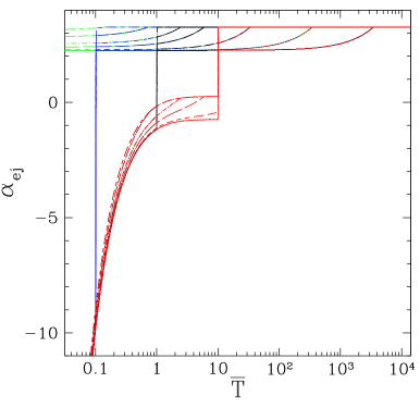
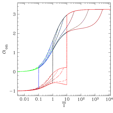
Figure 5: Evolution of the temporal indexes $\alpha_{ej}=-d\log F_{\nu}/d\log\tilde{T}$ (left panel) and $\alpha_{on}=-d\log F_{\nu}/d\log\bar{T}$ (right panel) with normalized observed time $\bar{T}$, at different observed photon energies (for $E_{0}=300\;{\rm keV}$). Different line styles are used for the different energies. The color coding shows the temporal indexes for several values of $\bar{T}_{f}=\Delta R/R_{0}$: $0$ (green), $0.1$ (blue), $1$ (black) and $10$ (red). The low and high energy spectral slopes are $b_{1}=-0.25$ and $b_{2}=-1.25$, while $a=1$.

Figure 5 shows the evolution of the temporal indexes $\alpha_{ej}$ and $\alpha_{on}$ during a pulse (See appendix B for the detailed evolution of the temporal and spectral slopes). The temporal index $\alpha_{ej}$ starts at very negative values and gradually increases, until at $\bar{T}_{f}$ it makes an abrupt jump to its value during the decaying part of the pulse, which is exactly $2+\beta$ (see eq. [B36]). The temporal index $\alpha_{on}$ starts at early times, $\bar{T}\ll 1$, either at $-1$ for $\bar{T}_{f}>0$ and $\bar{T}<\bar{T}_{f}$, or from $0$ for $\bar{T}_{f}\to 0$. Moreover, for $0<\bar{T}_{f}\ll 1$, $\alpha_{on}\approx-1$ for $\bar{T}<\bar{T}_{f}$ and $\alpha_{on}\approx 0$ for $\bar{T}_{f}<\bar{T}\ll 1$ (see eqs. [B8] and [B20]). Note that when $\alpha_{on}$ jumps from its negative value to a positive value at $\bar{T}=\bar{T}_{f}$ (i.e. at the peak of the spike), it reaches the same function of $\bar{T}$, independent of the time of the jump, $\bar{T}_{f}$, and therefore the same function also holds for $\bar{T}_{f}=\Delta R/R_{0}=0$ (see eqs. [B8] and [B20]). At late times, $\bar{T}\gg 1$ and $\bar{T}>\bar{T}_{f}$, the HLE relation is approached, $\alpha_{on}\approx 2-b_{2}$.

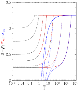
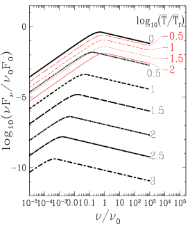
Figure 6: Left panel: Comparison of the evolution of the spectral ($\beta$ – thin lines) and temporal ($\alpha_{ej}$ – thick lines – and $\alpha_{on}$ – very thick lines) indexes at different photon energies ($E_{0}=300\;$keV). The low and high energy spectral slopes are $b_{1}=-0.25$ and $b_{2}=-1.25$, while $a=1$. Middle panel: Evolution of spectral index $\beta$ over the Swift XRT energy range ($\nu_{\rm min}<\nu<\nu_{\rm max}$ with $\nu_{\rm min}=0.2\;{\rm keV}$ and $\nu_{\rm max}=10]\;{\rm keV}$. Shown are the local values of $\beta$ at $\nu_{\rm min}$ (short dashed line), $\nu_{\rm max}/2$ (dotted line) and $\nu_{\rm max}$ (long dashed line), as well as the average values of $\beta$ over the XRT range, taken either over $\nu$ (thin solid line) or over $\log\nu$ (thick solid line). The low and high energy spectral slopes are $b_{1}=-0.25$ and $b_{2}=-1.25$, while $a=1$. Right panel: Evolution of the observed spectrum with time. The spectrum, $\nu F_{\nu}/(\nu_{0}F_{0})$, is shown as a function of the normalized frequency, $\nu/\nu_{0}$, for different values of the normalized time, $\log_{10}(\bar{T}/\bar{T_{f}})$, where we have used $\bar{T}_{f}=1$. The red thin lines correspond to the rising stage of the pulse $(\bar{T}<\bar{T}_{f})$, while the black thick lines are for its peak $(\bar{T}=\bar{T}_{f})$ and decaying stage $(\bar{T}>\bar{T}_{f})$. The low and high energy spectral slopes of the spectrum are $b_{1}=-0.25$ and $b_{2}=-1.25$, while $a=1$.

The left panel of figure 6 shows the evolution of $2+\beta$ (where $\beta$ is the spectral index) with the temporal indexes $\alpha_{ej}$ and $\alpha_{on}$. The spectral index naturally softens ($\beta$ increases with time), similar to what is typically observed (at least qualitatively), until it reaches $-b_{2}$ at late times ($\bar{T}\geq x_{b}\nu_{0}/\nu-1$). The change in $\beta$ occurs earlier at higher photon energies. At $\bar{T}\geq\bar{T}_{f}$, $\alpha_{ej}=2+\beta$ while $\alpha_{on}$ only approaches $2+\beta$ at late times.

In order to get a better idea of how the observed spectral index $\beta$ is expected to behave in Swift XRT observations, we calculate its average values over the XRT energy range (0.2–10 keV). We define two average values, by integrating over either the frequency $\nu$ or its logarithm $\log\nu$:

$$\langle\beta\rangle_{\nu}\equiv\frac{1}{(\nu_{\rm max}-\nu_{\rm min})}\int_{\nu_{\rm min}}^{\nu_{\rm max}}d\nu\,\beta(\nu)\ ,\qquad\qquad\langle\beta\rangle_{\log\nu}\equiv\frac{1}{\log(\nu_{\rm max}/\nu_{\rm min})}\int_{\nu_{\rm min}}^{\nu_{\rm max}}\frac{d\nu}{\nu}\,\beta(\nu)=-\frac{\log(F_{\nu_{\rm max}}/F_{\nu_{\rm min}})}{\log(\nu_{\rm max}/\nu_{\rm min})}\ .$$ (19)

The middle panel of figure 6 shows the evolution of these two averages as well as the values of $\beta$ at $\nu_{\rm min}=0.2\;$keV, $\nu_{\rm max}/2=5\;$keV and $\nu_{\rm max}=10\;$keV. As expected, $\langle\beta\rangle_{\nu}$ gives a larger weight to higher frequencies compared to $\langle\beta\rangle_{\log\nu}$, and its value it is usually very close to the spectral slope at $\nu_{\rm max}/2$ ($5\;$keV), except when the break frequency $\nu_{p}$ of the Band spectrum passes through the XRT range, and the change in $\beta$ within this range is the largest. Therefore, $\langle\beta\rangle_{\log\nu}$ appears to better reflect the spectral slope measured over a finite frequency range.

4.2 Spectrum

The local spectral emissivity in the comoving frame is taken to be a Band function. We have seen previously that for the parameter values relevant for internal shocks ($m=0$, $d=-1$), the observed spectrum is also a pure Band function. This is evident in the right panel of figure 6, which shows the temporal evolution of the observed spectrum in our model. It results from the fact that for these parameter values the observed peak frequency $\nu_{p}$ is constant along the EATS. We have $\nu_{p}/\nu_{0}=E_{p}(T)/E_{0}=1/\tilde{T}=1/(1+\bar{T})$ (see eq. (A24)) which is independent of $\bar{T}_{f}$. This behaviour is evident in the right panel of figure 6, where $E_{p}/E_{0}$ is $1$ at the onset of the spike ($\bar{T}=0$), $E_{p}/E_{0}=1/2$ at the peak of the spike ($\bar{T}=\bar{T}_{f}=1$), and $E_{p}/E_{0}$ decreases roughly linearly with $\bar{T}$ at later times, during the tail of the pulse.

5 Combining pulses to obtain the prompt emission

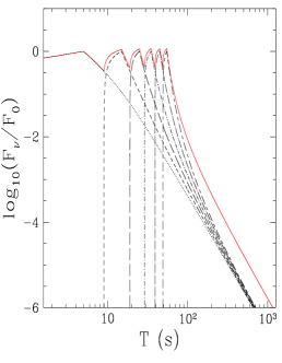
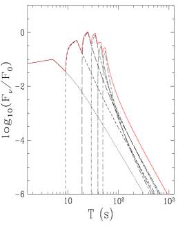
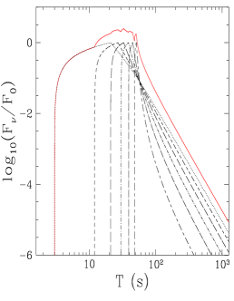
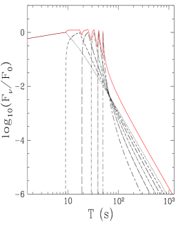
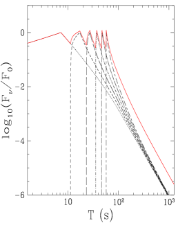
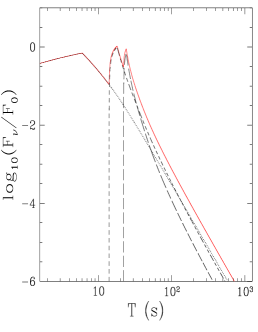
Figure 7: For all panels, The black lines show the individual pulses, while the red line shows the total prompt emission. The normalized observed frequency is $\nu/\nu_{0}=0.1$ (a): Prompt emission with six pulses, all having the same following parameters: $m=0$, $d=-1$, $a=1$, $b_{1}=-0.25$, $b_{2}=-1.25$, $T_{0}=2\;$s, $\bar{T}_{f}=\Delta R/R_{0}=3$ and $F_{\rm peak}/F_{0}=1$. The ejection times $T_{\rm ej}$ are (from the first to the last pulse): $-2\;$s, $8\;$s, $18\;$s, $28\;$s, $38\;$s and $48\;$s. (b): Same as top left panel, except for varying $F_{peak}/F_{0}$, which is from the first to the last pulse: $0.1$, $0.5$, $1$, $0.8$, $0.3$, and $0.2$. (c): Same as top left panel except for varying $T_{0}$ while $\Delta R/R_{0}=3$ remains constant, whose values are (from first to last pulse): $6\;$s, $5\;$s, $4\;$s, $3\;$s, $2\;$s, $1\;$s, which correspond to $T_{f}=$ $24\;$s, $20\;$s, $16\;$s, $12\;$s, $8\;$s, $4\;$s. To keep $t_{ej,1}=-T_{0,1}$ the ejection times in this case are: $-6\;$s, $4\;$s, $14\;$s, $24\;$s, $34\;$s and $44\;$s. (d): Same as top left panel except for varying $\Delta R/R_{0}$ while keeping $R_{0}$ and therefore $T_{0}$ constant. The values of $\Delta R/R_{0}$ are (from first to last pulse): $5$, $4$, $3$, $2$, $1$, $0$. Since $T_{0}=2\;$s, this corresponds to $T_{f}=(1+\Delta R/R_{0})T_{0}=$ $12\;$s, $10\;$s, $8\;$s, $6\;$s, $4\;$s, and $2\;$s, respectively. (e): Same as top left panel except for varying $\Delta R/R_{0}$ while keeping $R_{f}$ constant and therefore $T_{f}$ and $T_{0}/R_{0}$ also remain constant, while both $R_{0}$ and $T_{0}$ vary. From first to last pulse, $\Delta R/R_{0}=$ $10$, $3$, $1$, $0.3$, $0.1$, and $0.03$, and since $T_{f}=8\;$s this corresponds to $T_{0}=$ $0.727\;$s, $2\;$s, $4\;$s, $6.15\;$s, $7.27\;$s, and $7.77\;$s. The final peak frequency $\nu_{p}(\tilde{T}_{f})=(T_{0}/T_{f})\nu_{0}$ at $T_{f}$ is also kept constant, so that from the first to the last pulse $\nu/\nu_{0}=$ $0.0091$, $0.025$, $0.05$, $0.0769$, $0.0909$, $0.0971$. (f): example of a more realistic prompt emission consisting of three pulses with $T_{\rm ej}=-1\;$s, $13\;$s, $21\;$s, $T_{0}=2\;$s for all three pulses, $\Delta R/R_{0}=3$, $2$, $1$, and $F_{\rm peak}/F_{0}=0.7$, $1$, $0.7$.

There is good observational evidence that the steep decay phase is the tail of the prompt emission (O’Brien et al. 2006). Within our model, the prompt emission is the sum over a finite number of pulses, and therefore the steep decay phase is the sum of their tails. In this section we provide examples of combining several pulses to model the prompt emission, and study the effect of varying the different pulse parameters. To this end, we start with a simple prompt emission model consisting of six pulses that are identical except for their ejection time $T_{\rm ej}$ (see Fig. 7a). Each pulse corresponds to a single emission episode of a particular shell that was ejected at $T_{{\rm ej},i}$ (for $i$’th pulse), has an initial radial time $T_{0,i}$, and a final angular time of $T_{f,i}$. Then, we study the effect of changing the other model parameters one by one among the pulses. All lightcurves in this section are drawn against $T$, as the ejection time is different for each pulse (and then the definition of a $\tilde{T}$ $\bar{T}$ would differ for each pulse). In Fig. 7b the peak flux $F_{\rm peak}$ is varied. Next, we vary $T_{0}$ and/or $T_{f}$. In Fig. 7c, $T_{0}$ is varied while $T_{f}/T_{0}$ remains constant. In Fig. 7d, $T_{f}$ and $\Delta R/R_{0}$ vary while $T_{0}$ and $R_{0}$ remain constant. In Fig. 7e, $T_{0}$ and $\Delta R/R_{0}$ vary while $T_{f}$ and $R_{f}$ remain constant. Each of these panels show the light curve in logarithmic scales, $T=0$ is set to the onset time of the first pulse, which means that $T_{\rm ej,1}=-T_{0,1}$, thus showing the modeled prompt from a time close to what would be the trigger time for an observed burst. The red solid line represents the total prompt emission (the sum of all the pulses), while the black non solid lines are the individual underlying pulses. All the examples shown here of the prompt emission are for $\nu/\nu_{0}=0.1$.

In the case of six equal pulses (Fig. 7a), later pulses appear to decay much more steeply just after their peak in a logarithmic scale with the zero time near the beginning of the first pulse. At very late times the relative contribution from the different pulses becomes almost the same. As the only parameter that varies between pulses is the ejection time, $T_{\rm ej}$, this change in slope must depend only on it. Noting that the temporal slope is $\alpha\equiv-d\log F_{\nu}/d\log T=\alpha_{ej}/(1-T_{\rm ej}/T)$, and that the value of $\alpha_{ej}$ just after the peak is independent of $T_{\rm ej}$ (it depends only on $\tilde{T}_{f}$; see eq. [B32]), we can see that the value of $\alpha$ just after the peak scales as $\alpha_{\rm peak}=\alpha_{ej,{\rm peak}}(1+T_{\rm ej}/T_{f})$, since $T=T_{\rm ej}+T_{f}$ is the time of the peak of the pulse. Since the pulses are equal they have the same $T_{f}$ and $\alpha_{ej,{\rm peak}}$, it is clear that $\alpha_{\rm peak}$ increases with $T_{\rm ej}$. At late times when $T\gg T_{\rm ej}$, $\alpha$ approaches $\alpha_{ej}=2+\beta$.

When varying $F_{\rm peak}$ while fixing the other parameters (see Fig. 7b), the relative flux from each pulse at very late times is proportional to its $F_{\rm peak}$, so that the largest contribution is from the pulse with the largest $F_{\rm peak}$.

At late times the observed flux density of a single spike scales as $F_{\nu}\propto\tilde{T}^{\,b_{2}-2}$ (see, e.g., eq. [13]). If at the peak time of the spike, which for simplicity is assumed here to be at $T=T_{\rm ej}+T_{f}$ (as is usually the case), the observed photon energy is at the high-energy part of the Band function, $E\geq E_{*}\equiv E_{0}(T_{0}/T_{f})x_{b}$ or $\nu\geq\nu_{*}\equiv\nu_{0}(T_{0}/T_{f})x_{b}$, then (using eq. [13]) the flux from the peak onwards is simply given by

$$F_{\nu\geq\nu_{*}}(T\geq T_{\rm ej}+T_{f})=F_{\nu,{\rm peak}}\left(\frac{T-T_{\rm ej}}{T_{f}}\right)^{b_{2}-2}\ ,$$ (20)

while for $E/E_{*}=\nu/\nu_{*}<1$ the expression is slightly more complicated,

$$\frac{F_{\nu<\nu_{*}}}{F_{\nu,{\rm peak}}}=\left\{\begin{array}[]{ll}\left(\frac{T-T_{\rm ej}}{T_{f}}\right)^{b_{1}-2}e^{-(1+b_{1})(\nu/\nu_{0})(T-T_{\rm ej}-T_{f})/T_{0}}&T_{f}\leq T-T_{\rm ej}\leq T_{0}x_{b}\nu_{0}/\nu\ ,\\ \\ \left(\frac{T_{0}x_{b}\nu_{0}}{T_{f}\nu}\right)^{b_{1}-b_{2}}e^{b_{2}-b_{1}+(1+b_{1})(T_{f}/T_{0})(\nu/\nu_{0})}\left(\frac{T-T_{\rm ej}}{T_{f}}\right)^{b_{2}-2}&T-T_{\rm ej}\geq T_{0}x_{b}\nu_{0}/\nu\ ,\end{array}\right.$$ (21)

but the qualitative behaviour is still rather similar. Therefore, the flux ratio of two pulses with ejection times $T_{\rm ej,1}\leq T_{\rm ej,2}$ and a comparable $E_{p}(\bar{T}_{f})=(T_{0}/T_{f})E_{0}$ (as is usually the case for different pulses in the prompt emission of the same GRB), at late times ($T>\max(T_{\rm ej,1}+T_{f,1},T_{\rm ej,2}+T_{f,2})$ and $T-T_{\rm ej,2}\gg T_{\rm ej,2}-T_{\rm ej,1}$) is approximately

$$\frac{F_{\nu,1}(T)}{F_{\nu,2}(T)}\sim\frac{F_{\rm peak,1}}{F_{\rm peak,2}}\left(\frac{T_{f,1}}{T_{f,2}}\right)^{2+\beta}\ ,\quad{\rm for}\ \ \min[\bar{T}_{f,1},\bar{T}_{f,2}]>1\ \ {\rm and}\ \ T-T_{\rm ej,2}\gg T_{\rm ej,2}-T_{\rm ej,1}\ ,$$ (22)

where $\beta=-b_{2}$ for $\nu\geq\nu_{*}$ while $\beta$ is generally intermediate between $-b_{2}$ and $-b_{1}$ for $\nu<\nu_{*}$.

Fig. 7c demonstrates this nicely for a series of six pulses with the same $F_{\rm peak}$ but decreasing $T_{f}$, so that the later pulses with a smaller $T_{f}$ decay faster and become sub-dominant at late times. At the latest times the first spike, which has the largest $T_{f}$, dominates the observed flux in the tail emission. A similar behaviour is also seen in Fig. 7d. In Fig. 7e both $F_{\rm peak}$ and $T_{f}$ are the same between the different pulses, and therefore their tail fluxes at late times are similar. In Fig. 7c, $T_{0}$ and $T_{f}$ are varied while $T_{f}/T_{0}$ is constant, and it can be seen that this corresponds to a rescaling of the pulse width (its typical duration) without effecting its shape. In Fig. 7d, $T_{f}$ and $T_{f}/T_{0}$ are varied while $T_{0}$ is constant, and this nicely demonstrates how the shape of the pulse depends on $T_{f}/T_{0}$. Typically, the rise time of a pulse is $T_{f}-T_{0}$ while its decay time is $T_{f}$, so that the ratio of the rise and decay time is $1-T_{0}/T_{f}$. In Fig. 7e, $T_{0}$ and $T_{f}/T_{0}$ are varied while $T_{f}$ is constant. In this case the rise time varies considerably between the different pulses while the decay timescale and the late time tail of the pulses are practically the same. This arises since the tail is dominated by emission from $R\sim R_{f}$, that in this case is very similar for all the pulses. Moreover, for the particular choice of parameters in Fig. 7e, where $E_{p}(\bar{T}_{f})=(T_{0}/T_{f})E_{0}$ and $E_{*}=x_{b}E_{p}(\bar{T}_{f})$ remain constant for all the pulses, their late time tails have the same flux normalization. This can be understood from eq. (21), where the flux for $\tilde{T}>\max(\tilde{T}_{f},x_{b}\nu_{0}/\nu)$ can be written as $F_{\nu}/F_{\nu,{\rm peak}}=(E/E_{*})^{b_{2}-b_{1}}\exp[(b_{1}-b_{2})(E-E_{*})/E_{*}]\tilde{T}^{\,b_{2}-2}$.

Fig. 7f shows a more realistic example of the prompt emission, in which a larger number of model parameters is varied between the different pulses. This example contains only three pulses in order to be clearer. It can be seen that the flux during the decaying phase is initially dominated by the last pulse just after its peak ($T>27\;$s), but the second peak becomes dominant (even if only by a small factor) as early as $T\sim 37\;$s, and finally at $T\sim 140\;$s the first pulse becomes the dominant one. This demonstrates that different pulses can dominate the observed flux during the course of the steep decay phase. Which pulses would contribute more to the steep decay phase can be estimated according to their typical width (or duration), peak flux, and peak time. The peak time is most important at the beginning of the steep decay phase, where the last spike always dominates just after its peak if its peak is above the flux from the other spikes. Later on the relative contribution of the different spikes can be estimated according to eq. (22). Since the late time flux scales as $F_{\rm peak}T_{f}^{2+\beta}$ and usually $0\lesssim\beta\lesssim 2$, the power of $T_{f}$ (which corresponds to the typical width of the spike) is higher than that of $F_{\rm peak}$, so that wider spikes tend to dominate over narrower spikes, even if their peak flux is somewhat lower.

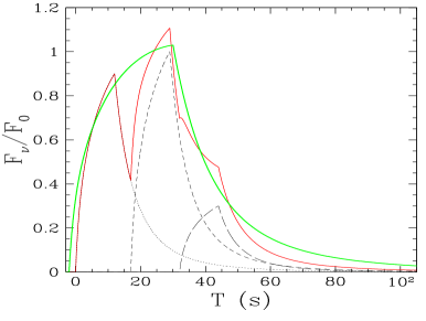
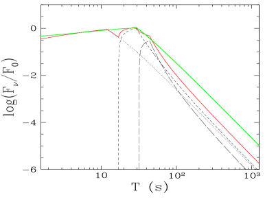
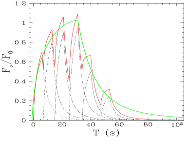
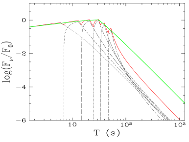
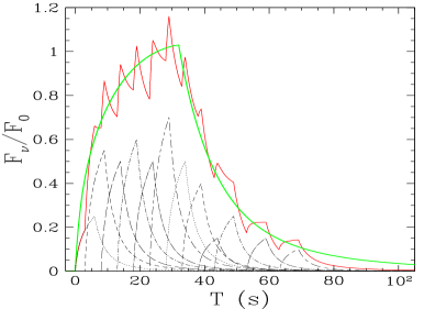
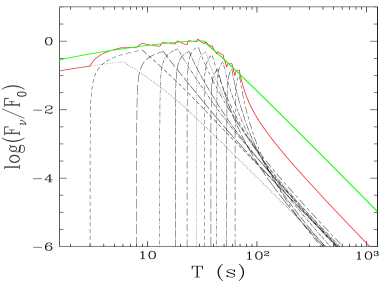
Figure 8: Comparison between the emission from several partially temporally overlapping pulses (individual pulses are in non-solid black lines, while the total prompt emission is in a solid red line), and a tentative fit to these pulses using a single broad pulse (thick solid green line). The same single broad pulse is used as a tentative fit for three different prompt emissions, with $3$ (top panels), $6$ (middle panels) and $12$ (bottom panels) pulses. The parameters of the pulses are shown tables 1, 2 and 3. The normalized observed frequency is $\nu/\nu_{0}=0.1$ Left panels: linear scale. Right panels: Logarithmic scale.

One should be very careful when fitting actual data with such a model. Fig. 8 shows what can happen if because of noisy data or coarse time bins, a prompt emission (red solid line) which is actually composed by several pulses (three, six or twelve in the cases shown; black non-solid lines) is fitted by a single broad pulse (green solid line). In this case the tail of the prompt emission can be significantly overestimated at late times, by a factor that tends to increase with the true number of underlying pulses. This can be understood by the simple example of comparing a single spike with $N$ identical spikes with the same peak flux but a duration smaller by a factor of $N$, for which the sum of their late time tail flux would be smaller than that of the single pulse by a factor of $\sim N^{1+\beta}$. However, in more realistic examples, the late time flux would often be dominated by the widest underlying pulse, so that its width would be more important than the total number of narrower underlying spikes. It is important to keep this effect in mind when confronting such a model with actual data.

6 Discussion and conclusions

We have presented and explored a model for the prompt GRB emission and its high latitude emission (HLE) tail. This model is physically motivated and realistic: it consists of a finite number of emission episodes, each of which corresponds to a single spike in the prompt light curve, and is modeled by a relativistically expanding thin spherical uniform shell emitting isotropically in its own rest frame within a finite range of radii. Our model thus describes the prompt emission and the steep decay pahse as a whole from its very start to its late tail. Yet this model is easy to use (fully analytic in its simplest form described here), making it particularly suitable for detailed combined temporal and spectral global fits to the prompt GRB emission and the following steep decay phase (SDP). Such fits can provide a stricter test of the HLE model for the SDP compared to most previous models, since we use a single self-consistent model to fit both the prompt emission and the SDP, while most previous models fit only the SDP and are largely decoupled from the details of the prompt emission. Moreover, our model is also physically motivated, and more realistic than previous models. We have derived analytic expressions for the flux in the realistic case of a Band function spectrum (eqs. [12] and [13]), which consists of two power laws that smoothly join at some typical photon energy.

The temporal evolution of the instantaneous values of the temporal ($\alpha$) and spectral ($\beta$) indexes for a single emission episode was studied, corresponding to a single observed pulse in the light curve. The definition of $\alpha$ is not unique as it depends on the choice of reference time. We explored two options for the reference time, either the ejection time ($\alpha_{ej}$) or the onset time of the spike ($\alpha_{on}$), and found that for the former the HLE relation ($\alpha_{ej}=2+\beta$) is satisfied from immediately after the peak of the spike ($\bar{T}>\bar{T}_{f}$), while for the former it is only approached at late times ($\alpha_{on}\approx 2+\beta$ at for $\bar{T}>\bar{T}_{f}$ and $\bar{T}\gg 1$).

We have intentionally chosen a simple model to describe the pulses, in order to reduce the number of free parameters. For a single emission episode (or pulse), in the most generic case there are ten free parameters: the power $m=-2d\log\Gamma/d\log R$, $d=d\log\nu^{\prime}_{p}/d\log R$, $a=d\log L^{\prime}_{\nu^{\prime}_{p}}/d\log R$, the normalization factor $F_{0}$ (or $L_{0}$), three additional parameters for the Band function (the two spectral slopes, $b_{1}$ and $b_{2}$, as well as the peak energy at the onset of the pulse $E_{0}$), the two timescales $T_{0}$ and $T_{f}$, and the ejection time $T_{\rm ej}$. We have the general constraint $\Delta R>0$, which implies $\tilde{T}_{f}=1+\Delta R/R_{0}>1$. Focusing on the internal shocks model fixes some of these parameters: as the outflow is typically in the coasting phase, $m=0$, while for synchrotron emission from fast cooling electrons $d=-1$ and $a=1$. Since we expect $\Delta R/R_{0}=\bar{T}_{f}\sim 1$ we can fix $\bar{T}_{f}\sim 1$ (although a wider range, such as $0.2\Delta R/R_{0}\lesssim 5$, may still be considered as plausible). Fixing $m$, $d$, $a$, and $T_{f}/T_{0}$ in this manner would leave only six free parameters. For a prompt emission with several pulses, one may be able in some cases to neglect the spectral evolution and use the same values of $b_{1}$, $b_{2}$, and $E_{0}$ for all the different pulses (or at least two of them, e.g. $b_{1}$ and $b_{2}$), which leads to a total number of free parameter of $3(N_{\rm pulses}+1)$ (or $4N_{\rm pulses}+2$ if $E_{0}$ cannot be fixed for all the pulses) for a burst with $N_{\rm pulses}$ pulses.

The shape of the pulses in our model can vary considerably, from very spiky peaks to rounder ones, from a very sharp rise to shallower rise, and so on (see Figs. 2 – 4). This can help reproduce some of the observed diversity in the shape of spike in the prompt light curve. This appears to be a promising feature of our model. However, we have an abrupt change in the temporal index at $\bar{T_{f}}$, that usually corresponds to a sharp peak of the spike. This is caused by our model assumption that the emission abruptly shuts off at the outer emission radius $R_{f}$. Therefore, we also consider an alternative and more realistic assumption, which leads to a rounder peak for the spikes, where the emission more gradually turns off at $R>R_{f}$. This is done by introducing and exponential turn-off with radius of the comoving spectral luminosity, $L^{\prime}_{\nu^{\prime}}(R)$, and is examined in Appendix C. The more gradual the turn-off of the emission with radius the rounder the peak of the pulse in the light curve. This can help fit the observed variety of pulse shapes even better (at the cost of adding an additional free parameter).

In the particular case of synchrotron emission from internal shocks, we find that the observed spectrum has the same shape as the emitted one, which in our case is modeled as a Band function. The observed peak photon energy of the Band function decreases with time, $E_{p}(\tilde{T})=E_{0}/\tilde{T}$, naturally leading to a softening of the spectrum with time, similar to what is observed by Swift. Thus, our model can at least qualitatively reproduce the main temporal and spectral features observed by Swift. The spectral index $\beta$ evolves from its value below $E_{p}$ ($\beta=-b_{1}$) to its value above $E_{p}$ ($\beta=-b_{2}$), where the transition that corresponds to the passage of $E_{p}$ through the observed energy band occurs at earlier times for higher observed photon energies (or frequencies).

When modeling the prompt emission by combining several pulses, the SDP is initially dominated by the last pulse (just after its peak, if it is above the flux fro the other pulses), but can later be dominated by the tail of other pulses. The relative contribution of a pulse to the late time flux scales as $\sim F_{peak}T_{f}^{2+\beta}$, and therefore wider pulses (with a larger $T_{f}$), and to a lesser extent pulses with a larger peak flux ($F_{\rm peak}$), tend to dominate the late time flux, deep into the SDP. Moreover, often the contribution to the total flux from the tails of several pulses can be comparable, so it cannot be adequately modeled using a single pulse model. Therefore, we caution here that modeling the steep decay phase using the HLE of a single pulse, $F_{\nu}\propto(T-T_{\rm ref})^{-(2+\beta)}$, may lead to wrong conclusions, and all the more so if the reference time $T_{\rm ref}$ is arbitrarily set to the GRB trigger time. Even if $T_{\rm ref}$ is set to the onset time of the last spike, this may still be a bad approximation in many cases since (i) we find that $\alpha_{ej}=2+\beta$ (with $T_{\rm ref}=T_{\rm ej}$) rather than $\alpha_{on}$ (with $T_{\rm ref}=T_{\rm ej}+T_{0}$, corresponding to the onset of the spike) while $\alpha_{on}$ approaches $\alpha_{ej}=2+\beta$ only at late times well after the peak of the last pulse, and (ii) at such late times the flux often becomes dominated by the tails of earlier pulses.

Our model can produce different shapes for the tail of the prompt emission, from close to a power law (which can have a different temporal index than its asymptotic late time value) to a curved shape with decreasing temporal index $\alpha$. This is qualitatively consistent with observations, where these type of behaviour are observed. We have demonstrated that just after the peak of the last pulse, the decay index of the prompt emission tail can reach very large values, far greater than the typical average value observed during the SDP by Swift, of $3\lesssim\alpha\lesssim 5$ (Nousek et al. 2006). Larger values for the temporal index, however, are sometimes observed close to the end of the prompt emission (for example in GRB050422, GRB050803 or GRB050916; see figure 2 from O’Brien et al. 2006), in accord with our model.

Because of the large number of free parameters, the fitting of actual data should be handled with care, and there may be various degeneracies involved. The results of such fits to data should also be taken cautiously because of the difficulty in properly resolving distinct pulses in the prompt emission. For different reasons (such as noisy data, coarse time bins, pulse overlap, etc.), a group of distinct pulses may be fitted by a single broader pulse, resulting in an over-prediction of the flux during the SDP, as well different spectral and temporal evolution, which might lead to a misinterpretation of the SDP. Nevertheless, when handled with care, a fit of our model to a good combined data set of the prompt GRB emission and its SDP tail can serve as a powerful test of the HLE model for the SDP, and thus help distinguish between different models for the prompt GRB emission.

J. G. gratefully acknowledges a Royal Society Wolfson Research Merit Award.

pulse number	1	2	3	broad pulse
$T_{\rm ej}$ [s]	-2	15	35	-4
$T_{0}$ [s]	2	4	5	4
$T_{f}$	16	16	25	36
$F_{\rm peak}/F_{0}$	0.85	1	0.12	1.03

Table 1: Parameters of the pulses for figure 8 (top panels)

pulse number	1	2	3	4	5	6	broad pulse
$T_{\rm ej}$ [s]	-2	1	16	26	36	46	-4
$T_{0}$ [s]	2	2	2	1.5	2	2	4
$T_{f}$	6	10	6	6	8	8	36
$F_{\rm peak}/F_{0}$	0.25	0.8	0.9	1	0.4	0.2	1.03

Table 2: Parameters of the pulses for figure 8 (middle panels)

pulse number	1	2	3	4	5	6	7	8	9	10	11	12	broad pulse
$T_{\rm ej}$ [s]	-2	-1	5	11	19	20	26	31	36	44	51	66	-4
$T_{0}$ [s]	2	2	2	2	1	2	2	2	3	2	2	3	4
$T_{f}$	4	6	6	6	2	5	6	6	7.5	8	6	6	36
$F_{\rm peak}/F_{0}$	0.25	0.5	0.75	0.85	0.75	0.85	0.95	0.55	0.35	0.25	0.11	0.11	1.03

Table 3: Parameters of the pulses for figure 8 (bottom panels)

Figure 2: Lightcurves of a single pulse at different normalized frequencies, $\nu/\nu_{0}$. The low and high energy slopes of the spectrum are $b_{1}=-0.25$ and $b_{2}=-1.25$, while $a=1$. $\Delta R/R_{0}=1$, so that $\tilde{T}_{f}=2$ and $\bar{T}_{f}=1$. Left: Normalized flux density shown as a function of $\tilde{T}$ in linear scale. Right: Flux density shown as a function of $\bar{T}$ in logarithmic scale.

Figure 3: The same pulse as in figure 2 is shown for different values of $\bar{T}_{f}$ for $(\nu/\nu_{0})=0.01$, $0.1$, and $1$ in the first, second and third panel respectively (in logarithmic scale). The fourth panel shows the case $(\nu/\nu_{0})=1$ in linear scale in order to show the shape of a pulse having its peak before $T=T_{f}$. The normalized flux density is shown as a function of $T\times T_{0,i}/T_{f_{i}}$ where the subscript $i$ denotes the $i$’th pulse, so that all the $T_{f,i}$ would appear to coincide, and the decay times of the different pulses would appear to be the same.

Figure 4: Effect of the variation of $a$ on the shape of a pulse for $(\nu/\nu_{0})=0.01$, $0.1$, and $1$ in the first, second and third panel respectively (in logarithmic scale). We can see that increasing $a$ makes the pulse sharper. The constant parameters are $T_{0}=1$ s and $T_{f}=2$ s and the low and high energy spectral slopes are $b_{1}=-0.25$ and $b_{2}=-1.25$.

In order to calculate the flux density $F_{\nu}$ that reaches the observer at an observed time $T$, we closely follow Granot, Cohen-Tanugi and DoCouto e Silva 2008: we integrate over the Equal Arrival Time Surface (EATS), i.e. the locus of points from which photons that are emitted by the shell at a radius $R$, angle $\theta$ relative to the line of sight, and a lab frame time $t$, reach the observer simultaneously at an observed time $T$. The lab frame time and the shell radius are related by

$$t-t_{\rm ej}=\int_{0}^{R}\frac{dr}{\beta c}\approx\frac{R}{c}+\frac{R}{2(m+1)c\Gamma^{2}}\ .$$ (A1)

From simple geometrical considerations, the EATS is given by

$$\frac{T-T_{\rm ej}}{(1+z)}=t-t_{\rm ej}-\frac{R\cos\theta}{c}\approx\frac{R}{c}\left[1-\cos\theta+\frac{1}{2(m+1)\Gamma^{2}}\right]\ ,$$ (A2)

Since $\Gamma\gg 1$ we can consider only small emission angles $\theta\ll 1$, for which $\cos\theta\approx 1-\theta^{2}/2$, so that the EATS reads

$$\frac{T-T_{\rm ej}}{(1+z)}\approx\frac{R_{L}}{2(m+1)c\Gamma_{L}^{2}}\left[y^{m+1}+y(m+1)(\Gamma_{L}\theta)^{2}\right]\ ,$$ (A3)

where we have introduced the normalized radius $y\equiv R/R_{L}$, as well as $R_{L}=R_{L}(T)$ that is the largest radius on the EATS at time $T$, and $\Gamma_{L}\equiv\Gamma(R_{L})$. Since $R_{L}$ is always obtained along the line of sight (at $\theta=0$),

$$R_{L}=2(m+1)c\Gamma_{L}^{2}\frac{T-T_{\rm ej}}{(1+z)}=R_{0}\left(\frac{T-T_{\rm ej}}{T_{0}}\right)^{\frac{1}{m+1}}\ ,\quad T_{0}=\frac{(1+z)R_{0}}{2(m+1)c\Gamma_{0}^{2}}\ .$$ (A4)

Substituting eq. (A4) into eq. (A3) implies

$$1-\mu\approx\frac{\theta^{2}}{2}=\frac{y^{-1}-y^{m}}{(m+1)\Gamma_{L}^{2}}\ ,\quad\frac{d\mu}{dy}=\frac{y^{-2}+my^{m-1}}{2(m+1)\Gamma_{L}^{2}}\ ,$$ (A5)

where $\mu\equiv\cos\theta$. The Doppler factor between the comoving frame and the lab frame is given by

$$\delta\equiv(1+z)\frac{\nu}{\nu^{\prime}}=\frac{1}{\Gamma(1-\beta\mu)}\approx\frac{2\Gamma}{1+(\Gamma\theta)^{2}}=\frac{2(m+1)\Gamma_{L}y^{-m/2}}{m+y^{-m-1}}\ .$$ (A6)

Remembering the reader that $T=T_{\rm ej}+T_{f}$ is the time at which the last photons that are emitted along the line of sight (from $R_{f}$ and $\theta=0$) reach the observer (which can be defined here by $R_{L}(T_{\rm ej}+T_{f})\equiv R_{f}$), from equation (A4) its general value is

$$T_{f}=T_{0}\left(\frac{R_{f}}{R_{0}}\right)^{m+1}=T_{0}\left(1+\frac{\Delta R}{R_{0}}\right)^{m+1}\ .$$ (A7)

In the limit $\Delta R\to 0$, $T_{f}\to T_{0}$.

The observed flux is then obtained by integration over the EATS (Sari 1998; Granot 2005),

$$F_{\nu}(T)=\frac{(1+z)}{4\pi d_{L}^{2}}\int dL_{\nu}=\frac{1+z}{4\pi d_{L}^{2}}\int\delta^{3}dL^{\prime}_{\nu^{\prime}}=\frac{1+z}{8\pi d_{L}^{2}}\int_{y_{\rm min}}^{y_{\rm max}}dy\,\frac{d\mu}{dy}\,\delta^{3}(y)\,L^{\prime}_{\nu^{\prime}}(y)\ ,$$ (A8)

where $dL^{\prime}_{\nu^{\prime}}=L^{\prime}_{\nu^{\prime}}(R)d\nu d\phi/4\pi\to L^{\prime}_{\nu^{\prime}}(r)d\mu/2=\frac{1}{2}L^{\prime}_{\nu^{\prime}}(R)(d\mu/dy)dy$ due to symmetry around the line of sight (no dependence of the emission on the azimuthal angle $\phi$), $L^{\prime}_{\nu^{\prime}}(R)$ is the total comoving spectral luminosity of the shell (the emitted energy per unit time and frequency), $\nu^{\prime}=\nu(1+z)/\delta$, and $d_{L}(z)$ is the luminosity distance of the source. The limits of integration over $y$ are

$$y_{\rm min} = \min\left(1,\frac{R_{0}}{R_{L}(T)}\right)=\left\{\begin{array}[]{ll}1&T\leq T_{\rm ej}+T_{0}\ ,\\ \left(\frac{T-T_{\rm ej}}{T_{0}}\right)^{-1/(m+1)}&T\geq T_{\rm ej}+T_{0}\ ,\\ \end{array}\right.,$$ (A11)

$$y_{\rm max} = \min\left(1,\frac{R_{0}+\Delta R}{R_{L}(T)}\right)=\left\{\begin{array}[]{ll}1&T\leq T_{\rm ej}+T_{f}\ ,\\ \left(\frac{T-T_{\rm ej}}{T_{f}}\right)^{-1/(m+1)}&T\geq T_{\rm ej}+T_{f}\ .\\ \end{array}\right.\ .$$ (A15)

For $T\leq T_{\rm ej}+T_{0}$ we have $R_{L}(T)\leq R_{0}$ and therefore $y_{\rm min}=y_{\rm max}=1$ and $F_{\nu}(T)=0$. This is since the EATS does not intersect the emission region for $R_{L}<R_{0}$, and only touches it at one point, $(R,\,\theta)=(R_{0},\,0)$, for $R_{L}=R_{0}$ ($T=T_{\rm ej}+T_{0}$). The observed flux becomes non-zero for $R_{L}>R_{0}$, corresponding to $T>T_{\rm ej}+T_{0}$. Substituting eqs. (A5) and (A6) into eq. (A8) finally gives

$$F_{\nu}(T)=\frac{(1+z)}{2\pi d_{L}^{2}}\,\Gamma_{0}\left(\frac{T-T_{\rm ej}}{T_{0}}\right)^{-m/[2(m+1)]}\int_{y_{\rm min}}^{y_{\rm max}}dy\,y^{-1-m/2}\left(\frac{m+1}{m+y^{-m-1}}\right)^{2}L^{\prime}_{\nu^{\prime}}(y)\ .$$ (A16)

A.1 Power-law spectrum

While a single power law emission spectrum is not very realistic, it already shows many important properties that also appear for a Band function emission spectrum (considered in the main text). This is the reason why this case is described here. The luminosity is then

$$L^{\prime}_{\nu^{\prime}}=L^{\prime}_{0}\left(\frac{R}{R_{0}}\right)^{a}\left(\frac{\nu^{\prime}}{\nu^{\prime}_{0}}\right)^{b}=L^{\prime}_{0}\tilde{T}^{(2a+mb)/[2(m+1)]}\left(\frac{\nu}{\nu_{0}}\right)^{b}y^{a+mb/2}\left(\frac{m+1}{m+y^{-m-1}}\right)^{-b}\ ,$$ (A17)

where the comoving spectral luminosity also scales as a power law with radius when the emission is over a finite range of radii, $\nu^{\prime}_{0}$ is a fixed frequency in the comoving frame.

A.1.1 Emission from an infinitely thin shell at radius $R_{0}$

We first study the case where the whole emission comes from a single radius $R_{0}$,

$$L^{\prime}_{\nu^{\prime}} = L^{\prime}_{0}\left(\frac{\nu^{\prime}}{\nu^{\prime}_{0}}\right)^{b}R_{0}\delta(R-R_{0})=L^{\prime}_{0}\left(\frac{\nu}{\nu_{0}}\right)^{b}\left(\frac{y}{y_{\rm min}}\right)^{mb/2}\left(\frac{m+1}{m+y^{-m-1}}\right)^{-b}y_{\rm min}\delta(y-y_{\rm min})$$ (A18)

$$= L^{\prime}_{0}\left(\frac{\nu}{\nu_{0}}\right)^{b}\left(\frac{m+1}{m+y_{\rm min}^{-m-1}}\right)^{-b}y_{\rm min}\delta(y-y_{\rm min})\ ,$$

where this is valid only for $\tilde{T}\geq 1$ that corresponds to $R_{L}\geq R_{0}$, for which $y_{\rm min}=R_{0}/R_{L}=[(T-T_{\rm ej})/T_{0}]^{-1/(m+1)}$. Eq. (A16) then implies

$$F_{\nu}(T\geq T_{\rm ej}+T_{0})=\frac{(1+z)}{4\pi d_{L}^{2}}L_{0}\left(\frac{\nu}{\nu_{0}}\right)^{b}\left[\frac{T-T_{\rm ej}+mT_{0}}{(m+1)T_{0}}\right]^{b-2}\ .$$ (A19)

There are two times of particular relevance here: the radial time $T_{r}(R_{0})=T_{0}=(1+z)R_{0}/[2c(m+1)\Gamma_{0}]$, which is the time past $T_{\rm ej}$ when the first photons start reaching the observer, and the angular time $T_{\theta}(R_{0})=(1+z)R_{0}/(2c\Gamma_{0})=(m+1)T_{r}(R_{0})$ that sets the time-scale for the width of the pulse. One can rewrite the expression for the observed flux density as

$$F_{\nu}(T>T_{\rm ej}+T_{0})=\frac{(1+z)}{4\pi d_{L}^{2}}L_{0}\left(\frac{\nu}{\nu_{0}}\right)^{b}\left[\frac{T-T_{s}}{T_{\theta}(R_{0})}\right]^{b-2}\ ,$$ (A20)

where $T_{s}=T_{\rm ej}+T_{0}-T_{\theta}(R_{0})=T_{\rm ej}-mT_{0}$ is the reference time for the power-law flux decay of the pulse, and is exactly $T_{\theta}(R_{0})$ before the onset of the pulse. Since the emission itself occurs at one particular radius ($R_{0}$) it depends only on the Lorentz factor at that radius radius, and is independent of $m$. In particular, $T_{\theta}(R_{0})=(m+1)T_{0}$ and the pulse peak flux are independent of $m$. The value of $m$ affects only the onset time of the pulse ($T=T_{\rm ej}+T_{0}$) and the reference time for the power law flux decay. For internal shocks we expect a coasting shell ($m=0$) for which $T_{s}=T_{\rm ej}$ and $T_{\theta}(R_{0})=T_{0}$. It can easily be seen that the HLE relation, $\alpha=2+\beta$ where $F_{\nu}\propto T^{-\alpha}\nu^{-\beta}$, is satisfied here as $\beta=-b$ and $\alpha=2-b=2+\beta$.

A.1.2 Emission from a region of finite width

We now turn to the case where the emission comes from a range of radii between $R_{0}$ and $R_{f}=R_{0}+\Delta R>R_{0}$. The comoving spectral luminosity in this case is $L^{\prime}_{\nu^{\prime}}=L^{\prime}_{0}\left(R/R_{0}\right)^{a}\left(\nu^{\prime}/\nu^{\prime}_{0}\right)^{b}$, and the flux density is given by (Granot, Cohen-Tanugi & do Couto e Silva 2008):

$$F_{\nu}(T)=\frac{(1+z)}{4\pi d_{L}^{2}}L_{0}\left(\frac{\nu}{\nu_{0}}\right)^{b}\tilde{T}^{\frac{2a-m(1-b)}{2(m+1)}}\int_{y_{\rm min}}^{y_{\rm max}}dy\,y^{a-1-m(1-b)/2}\left(\frac{m+1}{m+y^{-m-1}}\right)^{2-b}\ ,$$ (A21)

which, for internal shocks ($m=0$) becomes:

$$F_{\nu}(T\geq T_{\rm ej}+T_{0})=\frac{(1+z)}{4\pi d_{L}^{2}}\frac{L_{0}(\nu/\nu_{0})^{b}}{(2+a-b)}\tilde{T}^{b-2}\left[\min(\tilde{T},\tilde{T}_{f})^{2+a-b}-1\right]\ .$$ (A22)

It is therefore obvious that for $T\geqslant T_{\rm ej}+T_{f}$ the HLE relation is valid, where the reference time is the ejection time $T_{\rm ej}$, as in this case the spectral slope is $\beta=-b$ and the temporal slope is $\alpha=2-b=2+\beta$. In this sense a finite range of emission radii with $m=0$ is similar to emission from a single radius, as in both cases the HLE relation $\alpha=2+\beta$ is strictly valid immediately from $T\geq T_{\rm ej}+T_{f}$, for some reference time, though in the latter case the reference time for which this is valid is equal to the observed ejection time only for $m=0$. For emission from a finite range of radii with $m\neq 0$ the relation $\alpha=2+\beta$ is approached asymptotically at $T-T_{\rm ej}\gg T_{f}$.

A.2 Band function spectrum: general case and late time dependence

In the main text we have given the flux in the specific case of internal shocks, $m=0$ and $d=-1$. We derive here the flux for any values of the parameters $m$ and $d$.

A.3 Emission from a single radius

When the whole emission comes from a single radius $R_{0}$, the peak frequency is $\nu^{\prime}_{p}=\nu^{\prime}_{0}$, and the luminosity is thus

$$L^{\prime}_{\nu^{\prime}}=L^{\prime}_{0}S\left(\frac{\nu^{\prime}}{\nu^{\prime}_{p}}\right)R_{0}\delta(R-R_{0})=L^{\prime}_{0}S\left(\frac{\nu^{\prime}}{\nu^{\prime}_{p}}\right)y_{\rm min}\delta(y-y_{\rm min})\ ,$$ (A23)

Using this luminosity (eq. [A23]) in the integral for the flux (eq. [A16]) results in

$$F_{\nu}(T\geq T_{\rm ej}+T_{0})=\frac{(1+z)}{4\pi d_{L}^{2}}L_{0}\left[\frac{T-T_{s}}{T_{\theta}(R_{0})}\right]^{-2}S\left(\frac{\nu}{\nu_{p}(T)}\right)\ ,\quad\frac{\nu_{p}(T)}{\nu_{0}}=\frac{E_{p}(T)}{E_{0}}=\left[\frac{T-T_{s}}{T_{\theta}(R_{0})}\right]^{-1}\ ,$$ (A24)

where as in § A.1, $T_{s}\equiv T_{\rm ej}-mT_{0}$ is the reference time for the power-law flux decay of the pulse, $T_{\theta}(R_{0})=(m+1)T_{0}=(1+z)R_{0}/2c\Gamma_{0}^{2}$ is the angular time at $R_{0}$, and $E_{p}(T)=h\nu_{p}(T)$ is the photon energy corresponding to the peak of the Band function spectrum. Note that for $m=0$, $T_{s}=T_{\rm ej}$. One can express the argument of $S$ as

$$\frac{\nu}{\nu_{p}(T)}=\frac{E}{E_{p}(T)}=\frac{\nu}{\nu_{0}}\left[\frac{T-T_{s}}{T_{\theta}(R_{0})}\right]\ ,\quad\frac{\nu}{\nu_{0}}=\frac{E}{E_{0}}=\frac{(1+z)\nu}{2\Gamma_{0}\nu^{\prime}_{0}}\ .$$ (A25)

Reminding that $F_{s}\equiv L_{0}(1+z)/(4\pi d_{L}^{2})$, we then use the explicit expression for the Band function (eq. [3]) to express the observed flux as:

$$\frac{F_{\nu}(T\geq T_{\rm ej}+T_{0})}{F_{s}} = \left\{\begin{array}[]{ll}\left[\frac{T-T_{s}}{T_{\theta}(R_{0})}\right]^{b_{1}-2}\left(\frac{\nu}{\nu_{0}}\right)^{b_{1}}e^{(1+b_{1})[1-\frac{\nu}{\nu_{0}}(T-T_{s})/T_{\theta}(R_{0})]}&\frac{T-T_{s}}{T_{\theta}(R_{0})}\leqslant\frac{x_{b}}{\frac{\nu}{\nu_{0}}}\ ,\\ \\ \left[\frac{T-T_{s}}{T_{\theta}(R_{0})}\right]^{b_{2}-2}\left(\frac{\nu}{\nu_{0}}\right)^{b_{2}}x_{b}^{b_{1}-b_{2}}e^{1+b_{2}}&\frac{T-T_{s}}{T_{\theta}(R_{0})}\geqslant\frac{x_{b}}{\frac{\nu}{\nu_{0}}}\ .\end{array}\right.$$ (A29)

A.4 Emission from a range of radii

In the case of emission with a Band function spectrum over a finite range of radii, $R_{0}<R<R_{f}=R_{0}+\Delta R$, we remind that the comoving luminosity is:

$$L^{\prime}_{\nu^{\prime}}=L^{\prime}_{0}\left(\frac{R}{R_{0}}\right)^{a}S\left(\frac{\nu^{\prime}}{\nu^{\prime}_{p}(R)}\right)$$ (A30)

Introducing (A30) into (A16) we obtain the general expression of the flux:

$$\frac{F_{\nu}}{F_{s}} = y_{\rm min}^{-a+m/2}\int_{y_{\rm min}}^{y_{\rm max}}dy\,y^{a-1-m/2}\left(\frac{m+1}{m+y^{-m-1}}\right)^{2}S\left(\frac{\nu^{\prime}}{\nu^{\prime}_{p}}\right)$$

$$= \int_{1}^{\tilde{y}_{\rm max}}d\tilde{y}\,\tilde{y}^{a-1-m/2}\left(\frac{m+1}{m+y_{\rm min}^{-m-1}\tilde{y}^{-m-1}}\right)^{2}S\left(\frac{\nu^{\prime}}{\nu^{\prime}_{p}}\right)\ ,$$

where $\tilde{y}=y/y_{\rm min}$, $\tilde{y}_{\rm max}=\min[y_{\rm min}^{-1},(T_{f}/T_{0})^{1/(m+1)}]$, and

$$\frac{\nu^{\prime}}{\nu^{\prime}_{p}}=\frac{\nu}{\nu_{0}}\left(\frac{y}{y_{\rm min}}\right)^{m/2-d}\left(\frac{m+y^{-m-1}}{m+1}\right)=\frac{\nu}{\nu_{0}}\,\tilde{y}^{m/2-d}\left(\frac{m+y_{\rm min}^{-m-1}\tilde{y}^{-m-1}}{m+1}\right)\ ,$$ (A32)

and the expression for $\nu^{\prime}/\nu^{\prime}_{p}$ assumes that $\nu^{\prime}_{p}=\nu^{\prime}_{0}(R/R_{0})^{d}=\nu^{\prime}_{0}(y/y_{\rm min})^{d}$. At late times, $T-T_{\rm ej}\gg T_{f}$, we have $y\ll 1$, $\tilde{y}_{\rm max}=T_{f}/T_{0}$, and $\nu^{\prime}/\nu^{\prime}_{p}\approx(\nu/\nu_{0})\tilde{y}^{-1-d-m/2}y_{\rm min}^{-m-1}/(m+1)$ increases with time so that $S(\nu^{\prime}/\nu^{\prime}_{p})\propto(\nu^{\prime}/\nu^{\prime}_{p})^{b_{2}}$ and $F_{\nu}\propto(\nu/\nu_{0})^{b_{2}}y_{\rm min}^{(m+1)(2-b_{2})}=(\nu/\nu_{0})^{b_{2}}[(T-T_{\rm ej})/T_{0}]^{b_{2}-2}$, i.e. the HLE relation $\alpha=2+\beta$ is satisfied.

In the case for internal shocks, with $m=0$ and $d=-1$, $\nu^{\prime}/\nu^{\prime}_{p}$ becomes independent of $y$ and can be taken outside the integral ($\nu^{\prime}/\nu^{\prime}_{p}=(\nu/\nu_{0})/y_{\rm min}=(\nu/\nu_{0})\tilde{T}$), leading to the much simpler expression of the flux seen in the main text (eq. 12).

Appendix B Evolution of the temporal and spectral indexes

This appendix explicits the evolution of the temporal and spectral indexes with time.

B.0.1 Single emission radius

Where the luminosity is a delta function with radius at radius $R_{0}$, we obtain

$$\beta = \left\{\begin{array}[]{ll}-b_{1}+\tilde{T}(1+b_{1})\nu/\nu_{0}&\tilde{T}\leqslant x_{b}\nu_{0}/\nu\\ \\ -b_{2}&\tilde{T}\geqslant x_{b}\nu_{0}/\nu\end{array}\right.$$ (B4)

$$\alpha_{on} = \left\{\begin{array}[]{ll}(2-b_{1})\bar{T}/(1+\bar{T})+\bar{T}(1+b_{1})\nu/\nu_{0}&\bar{T}\leqslant x_{b}\nu_{0}/\nu-1\\ \\ (2-b_{2})\bar{T}/(1+\bar{T})&\bar{T}\geqslant x_{b}\nu_{0}/\nu-1\end{array}\right.$$ (B8)

$$\alpha_{ej} = \left\{\begin{array}[]{ll}2-b_{1}+\tilde{T}(1+b_{1})\nu/\nu_{0}&\tilde{T}\leqslant x_{b}\nu_{0}/\nu\\ \\ 2-b_{2}&\tilde{T}\geqslant x_{b}\nu_{0}/\nu\end{array}\right.$$ (B12)

We then have a very simple relation between $\alpha_{ej}$ and $\beta$: $\alpha_{ej}=2+\beta$, as expected at asymptotically late times for HLE, just that for $\alpha_{ej}$ it is satisfied all along for the local values of the temporal and spectral indexes. At late times $\alpha_{on}$ approaches $\alpha_{ej}$ and a similar relation approximately holds between $\alpha_{on}$ and $\beta$ ($\alpha_{on}\approx 2+\beta$).

B.0.2 Emission from a finite range of radii: $R_{0}<R<R_{f}$

In this case, the spectral index $\beta$ is still given by eq. (B4), while the two temporal indexes are:

$$\alpha_{on}=\left\{\begin{array}[]{ll}(2-b_{1})\frac{\bar{T}}{(1+\bar{T})}+\bar{T}(1+b_{1})\frac{\nu}{\nu_{0}}-(2+a)\frac{\bar{T}(1+\bar{T})^{1+a}}{(1+\bar{T})^{2+a}-1}&\bar{T}<\min(\Delta R/R_{0},x_{b}\nu_{0}/\nu-1)\ ,\\ \\ (2-b_{1})\frac{\bar{T}}{(1+\bar{T})}+\bar{T}(1+b_{1})\frac{\nu}{\nu_{0}}&\Delta R/R_{0}<\bar{T}<x_{b}\nu_{0}/\nu-1\ ,\\ \\ (2-b_{2})\frac{\bar{T}}{(1+\bar{T})}-(2+a)\frac{\bar{T}(1+\bar{T})^{1+a}}{(1+\bar{T})^{2+a}-1}&x_{b}\nu_{0}/\nu-1<\bar{T}<\Delta R/R_{0}\ ,\\ \\ (2-b_{2})\frac{\bar{T}}{(1+\bar{T})}&\bar{T}>\max(\Delta R/R_{0},x_{b}\nu_{0}/\nu-1)\ ,\\ \end{array}\right.$$ (B20)

which limits at very early and very late times are

$$\alpha_{on}\approx\left\{\begin{array}[]{ll}-1&\bar{T}\ll 1\ ,\\ \\ 2-b_{2}&\bar{T}\gg 1\ ,\\ \end{array}\right.$$ (B24)

and

$$\alpha_{ej}=\left\{\begin{array}[]{ll}2-b_{1}-(2+a)/(1-\tilde{T}^{-a-2})+\tilde{T}(1+b_{1})\nu/\nu_{0}&\tilde{T}<\min(R_{f}/R_{0},x_{b}\nu_{0}/\nu)\ ,\\ \\ 2-b_{1}+\tilde{T}(1+b_{1})\nu/\nu_{0}&R_{f}/R_{0}<\tilde{T}<x_{b}\nu_{0}/\nu\ ,\\ \\ 2-b_{2}-(2+a)/(1-\tilde{T}^{-a-2})&x_{b}\nu_{0}/\nu<\tilde{T}<R_{f}/R_{0}\ ,\\ \\ 2-b_{2}&\tilde{T}>\max(R_{f}/R_{0},x_{b}\nu_{0}/\nu)\ .\end{array}\right.$$ (B32)

According to equations (B4) and (B32) $\alpha_{ej}$ has a simple relation with $\beta$:

$$\alpha_{ej}=\left\{\begin{array}[]{ll}\beta+2-(2+a)/(1-\tilde{T}^{-a-2})&\tilde{T}<R_{f}/R_{0}\ \ (\bar{T}<\bar{T}_{f})\ ,\\ \\ \beta+2&\tilde{T}>R_{f}/R_{0}\ \ (\bar{T}>\bar{T}_{f})\ .\\ \end{array}\right.$$ (B36)

Note that in the limit $\bar{T}\to 0$ ($\tilde{T}\to 1$), at very early times, just after the onset of the spike, $\alpha_{ej}\to-\infty$ while $\alpha_{on}\to-1$. Moreover, the simple HLE relation, $\alpha_{ej}=2+\beta$, is valid as soon as $\tilde{T}>\tilde{T}_{f}$, for any value of $\tilde{T}_{f}$. This is a relation between the local values of $\alpha_{ej}$ and $\beta$, that hold as both change with time, and is strictly valid from $\tilde{T}>\tilde{T}_{f}$ only for $m=0$ and $d=-1$. For general values of $m$ or $d$ this local HLE relation would be valid only at late times, $\bar{T}\gg\bar{T}_{f}$. Note, however, that for alternative other definitions of the temporal index, such as $\alpha_{on}$, this relation is only approached at late time: $\alpha_{on}\approx 2+\beta$ for $\bar{T}>\bar{T}_{f}$ and $\bar{T}\gg 1$.

Appendix C Exponential turn-off of the emission with radius

Throughout the paper we have assumed that the emission abruptly turns off at $R_{f}$. This results in a sharp change in the temporal index at $\bar{T}_{f}$, which usually corresponds to a sharp peak for the pulses in the prompt GRB light curve. Observations sometimes show pulses with a round peak, which may be hard to fit with spiky theoretical spikes. Such rounder peaks for the pulses may be obtain within the framework of our model by introducing a more gradual turn-off of the emission at $R>R_{f}$. For convenience, we parameterize this here by assuming that the luminosity starts decreasing exponentially with radius at $R>R_{f}$. For simplicity we consider here only $\Delta R>0$, but the results are similar for $\Delta R=0$. Similarly, only the case for internal shock ($m=0$, $d=-1$) is considered here. Thus, we introduce the following comoving spectral luminosity:

$$L^{\prime}_{\nu^{\prime}}=\left\{\begin{array}[]{ll}L^{\prime}_{0}\left(\frac{R}{R_{0}}\right)^{a}S\left(\frac{\nu^{\prime}}{\nu^{\prime}_{p}}\right)&R_{0}\leqslant R\leqslant R_{f}\\ \\ L^{\prime}_{0}\left(\frac{R}{R_{0}}\right)^{a}S\left(\frac{\nu^{\prime}}{\nu^{\prime}_{p}}\right)e^{-\frac{q(R-R_{f})}{\Delta R}}&R>R_{f}\end{array}\right.$$ (C4)

where $q$ is the decay constant (a larger $q$ corresponds to a sharper turn-off of the emission).

For $1\leqslant\tilde{T}\leqslant\tilde{T}_{f}$ the observed flux is identical to that without introducing the gradual emission turn-off, and is therefore given by eq. (12),

$$F_{\nu}(\tilde{T}\geq\tilde{T}_{f})=F_{0}\tilde{T}^{-2}\left[\left(\min(\tilde{T},\tilde{T_{f}})\right)^{2+a}-1\right]S\left(\frac{\nu}{\nu_{0}}\tilde{T}\right)\ .$$ (C5)

The flux for $\tilde{T}>\tilde{T}_{f}$ is obtained by calculations very similar to those of section 3.2, and reads

$$F_{\nu}(\tilde{T}\geq\tilde{T}_{f}) = F_{0}\tilde{T}^{-2}S(\tilde{T}\nu/\nu_{0})\left[\tilde{T}_{f}^{2+a}-1+J(\tilde{T})\right]\ ,$$ (C6)

$$J(\tilde{T}) \equiv (2+a)\int_{\tilde{T}_{f}}^{\tilde{T}}d\tilde{y}\,\tilde{y}^{a+1}e^{-(\tilde{y}-\tilde{T}_{f})/Q}\ ,$$ (C7)

were $Q\equiv\Delta R/(qR_{0})$, and we remind the reader that $\tilde{y}=\tilde{T}y$ for $m=0$. The expression for the flux is thus very similar its form for an abrupt turn-off of the emission at $R_{f}$, but with the additional term $J(\tilde{T})$ that adds some flux at $\tilde{T}>\tilde{T}_{f}$ (representing the added contributions from $R>R_{f}$). For $a=1$ we have

$$J(\tilde{T},a=1)=6Q^{3}+6Q^{2}\tilde{T}_{f}+3Q\tilde{T}_{f}^{2}-e^{-(\tilde{T}-\tilde{T}_{f})/Q}\left(6Q^{3}+6Q^{2}\tilde{T}+3Q\tilde{T}^{2}\right)\ .$$ (C8)

At late times $J(\tilde{T},a=1)$ approaches a constant value,

$$J_{\infty}\equiv 6Q^{3}+6Q^{2}\tilde{T}_{f}+3Q\tilde{T}_{f}^{2}\sim\left\{\begin{array}[]{ll}6\left(\frac{\Delta R}{qR_{0}}\right)^{3}&q\ll\frac{\Delta R/R_{0}}{1+\Delta R/R_{0}}\\ 3\frac{\Delta R}{qR_{0}}\left(1+\frac{\Delta R}{R_{0}}\right)^{2}&q\gg\frac{\Delta R/R_{0}}{1+\Delta R/R_{0}}\end{array}\right.$$ (C11)

where we have replaced $Q$ and $\tilde{T}_{f}$ by their dependence on $q$ and $\Delta R/R_{0}$. Since $J(\tilde{T})$ appears in eq. (C6) in a sum with $\tilde{T}_{f}^{2+a}-1$, it will dominate the observed flux at late times if $J_{\infty}>\tilde{T}_{f}^{2+a}-1$ or equivalently if $q<q_{\rm crit}$ where $J_{\infty}(q_{\rm crit})\equiv\tilde{T}_{f}^{2+a}-1$.

The left panel of figure 9 shows $q_{crit}$ as a function of $\bar{T}_{f}=\Delta R/R_{0}$ for $a=1$, and it can be seen that the limiting values of $q_{\rm crit}$ are $1$ for $\bar{T}_{f}\ll 1$, and $(7+22^{1/2})^{1/3}+1+3/(7+22^{1/2})^{1/3}\approx 4.59$ for $\bar{T}_{f}\gg 1$, so that $q_{\rm crit}$ is always of order unity. Therefore, for $q\ll q_{\rm crit}\sim 1$ the late time flux is dominated by contributions from $R>R_{f}$, the peak of the pulse is rounder and the peak flux is higher compared to an abrupt turn-off of the emission with radius, which is approached in the opposite limit of $q\gg q_{\rm crit}\sim 1$. This can nicely be seen in the right panel of fig. 9, which shows the shape of a pulse for different values of $q$, including the limiting case of $q\to\infty$, which corresponds to an abrupt turn-off of the emission at $R_{f}$.

Such an exponential turn-off could therefore be useful when fitting our our model with data, in order to reproduce round-peaks pulses. Of course, one should be aware that this adds a free parameter ($q$ or $Q$), and might thus increases the degeneracy between the different fit parameters. Therefore, adding this extra model parameter should be done only when it is required by the data.

Figure 9: Left: Dependence of the critical decay index $q_{crit}$ of the exponential cut-off on $\bar{T}_{f}=\Delta R/R_{0}$, in semi-logarithmic scale. It is defined by $J_{\infty}(q_{crit})=\tilde{T}_{f}^{3}-1$, i.e. at late time, the contribution to the flux from the exponential cut-off is equal to the contribution from the emitting region between $R_{0}$ and $R_{f}$. Right: Comparison of the shape of pulses with and without the exponential turn-off of the luminosity for a ratio $\Delta R/R_{0}=1$ in logarithmic scale. The solid line shows the shape of the pulse for an abruptly stopping luminosity (no exponential turn-off), the other lines show the pulse shape for different values of the decay constant $q=0.1$ of the exponential turn-off.

References

- (1) Band D., et al., 1993, ApJ , 281
- (2) Barniol Duran R. & Kumar P., 2008, accepted by MNRAS, astro-ph/0806.1226v1
- (3) Barthelmy, S. D., et al. 2005, Space Sci. Rev. , 143
- (4) Burrows, D. B., et al. 2005a, Space Sci. Rev., , 164
- (5) Burrows D. N. et al. 2005b, Science, , 1833
- (6) Butler, N. R., & Kocevski, D. 2007, ApJ, , 407
- (7) Costa E., et al., 1997, Nature , 783
- (8) Dai Z.G., 2004, ApJ , 1000
- (9) De Pasquale M., et al., 2006, A & A , 813
- (10) Eichler D. & Granot J., 2006, ApJ, , L5
- (11) Falcone A. D., et al., 2006, ApJ, 641, 1010
- (12) Gehrels N., et al., 2004, ApJ , 1005
- (13) Genet F., Daigne F. & Mochkovitch R., 2007, MNRAS 381, 732
- (14) Granot J., 2005, ApJ , 1022
- (15) Granot J., 2007, Il Nuovo Cimento B, 121, 1073
- (16) Granot J., Cohen-Tanugi J. & do Couto e Silva E., 2008, ApJ , 92
- (17) Granot J., Königl A. & Piran T., 2006, MNRAS, , 1946
- (18) Granot J., Kumar P., 2006, MNRAS, , L13
- (19) Granot J., Piran T. & Sari R., 1999, ApJ , 679
- (20) Krimm, H. A., et al. 2007, ApJ, 665, 554
- (21) Kumar P. & Panaitescu A., 2000a, ApJL , L51
- (22) Kumar P. & Piran T., 2000, ApJ , 286
- (23) Lee W.H., Ramirez-Ruiz E., 2002, ApJ , L893
- (24) Liang E.W. et al., 2006, ApJ , 351
- (25) Lyutikov M. & Blandford, R.D., 2003, astro-ph/0312347v1
- (26) MacFadyen A.I., Woosley S.E. & Heger A., 2001, ApJ , 410
- (27) Mészaros P. & Rees M.J., 2001, ApJ , L37
- (28) Nousek J.A., et al., 2006, ApJ , 389
- (29) O’Brien P.T., et al., 2006, ApJ , 1213
- (30) Panaitescu A., et al., 2006, MNRAS , 1357
- (31) Peng F., Königl A. & Granot J., 2005, ApJ , 966
- (32) Preece R.D., et al., 2000, ApJS , 19
- (33) Qin Y.-P., 2008, ApJ , 900
- (34) Ramirez-Ruiz E., 2004, MNRAS , L38
- (35) Ramirez-Ruiz E., Celotti A & Rees M.J., 2002, MNRAS , 1349
- (36) Ramirez-Ruiz E., Merloni A. & Rees M.J., 2001, MNRAS , 1147
- (37) Rees M., 1966, Nature , 468
- (38) Rees M. & Mészaros P., 1994, ApJ , L93
- (39) Rees M. & Mészaros P., 1998, ApJ , L1
- (40) Rees M. & Mészaros P., 2000, ApJ , L73
- (41) Roming, P. W. A., et al. 2005, Space Sci. Rev., 120, 95
- (42) Sakamoto T., et al., 2007, ApJ , 1115
- (43) Sari, R. 1998, ApJ, 494, L49
- (44) Sari R. & Mészaros P., 2000, ApJ , L33
- (45) Sari R. & Piran T., 1997, ApJ , 270
- (46) Soffitta P., De Pasquale M., Piro L. & Costa E., 2004, proceedings of the Third Rome Workshop on Gamma-Ray Bursts in the Afterglow Era, ASP Conferences series, Vol. , M.Feroci, F.Frontera, N.Masetti & L.Piro eds.
- (47) Tagliaferri G, et al., 2005, Nature , 985
- (48) vanParadijs J., et al., 1997, Nature , 686
- (49) Yamazaki R., Toma K., Ioka K. & Nakamura T., 2006, MNRAS , 311
- (50) Zhang B.B, Liang E.W. & Zhang B., 2007, ApJ , 1002