Hepp and Speer Sectors within Modern Strategies of Sector Decomposition

A.V. Smirnov
Scientific Research Computing Center of Moscow State University

and

V.A. Smirnov
Nuclear Physics Institute of Moscow State University

Abstract

Hepp and Speer sectors were successfully used in the sixties and seventies for proving mathematical theorems on analytically or/and dimensionally regularized and renormalized Feynman integrals at Euclidean external momenta. We describe them within recently developed strategies of introducing iterative sector decompositions. We show that Speer sectors are reproduced within one of the existing strategies.

1 Introduction

The so-called alpha representation [1–11] was initially used to introduce dimensional regularization [12, 13] and to prove various mathematical results on Feynman integrals [3, 4, 5, 6, 8, 9, 10, 11]. The standard way to analyze convergence of Feynman integrals is to decompose the initial integration domain of alpha parameters into appropriate subdomains (sectors) and introduce, in each sector, new variables in such a way that the integrand factorizes, i.e. becomes equal to a monomial in new variables times a non-singular function. This procedure turned out to be successful for Euclidean external momenta, i.e with $\left(\sum q_{i}\right)^{2}<0$ for any partial sum, when the sectors of Hepp [3] and Speer [5] were introduced.

However, in practice, one often deals with Feynman integrals on a mass shell or at a threshold. In this case, Hepp or Speer sectors generally do not provide a factorization of the integrand so that the analysis of convergence fails within this technique. Therefore, general theorems on such ‘physical’ Feynman integrals could not be proved up to now.

Recently Binoth and Heinrich introduced sector decompositions of a new kind [14]. (See [15] for a review.) They provided a powerful method of evaluating Feynman integrals numerically in situations with severe UV, IR and collinear divergences. In contrast to Hepp and Speer sectors, the sectors of [14] are introduced iteratively, according to so-called sector decomposition strategies. The corresponding algorithm was implemented on a computer. Although this algorithm was successfully applied to numerically evaluate complicated Feynman integrals and to check existing analytical results (see, e.g. [16, 17, 18]) it was unclear where this iterative procedure stops at some point, i.e. results in the factorization of the integrands so that one can apply it for numerical evaluation. Indeed, in some examples, closed loops appear within this algorithm.

The first algorithm guaranteed to terminate was developed by Bogner and Weinzierl [19]. More precisely, certain strategies within this algorithm guarantee that closed loops do not appear. The algorithm works at least if squares $\left(\sum q_{i}\right)^{2}$ of partial sums of the external momenta are either negative or zero. (We will formulate a more general condition in the next section.) The corresponding computer code is public. The second public algorithm [20] called FIESTA provided one more strategy (Strategy S) for sector decompositions which also leads to a factorization of the integrand for general Feynman integrals. It was successfully applied in [21].

The purpose of this paper is to describe Hepp and Speer sectors in an iterative way, within the modern technique of sector decompositions. Using examples of three- and four-loop diagrams, we will also see that Speer sectors are reproduced within Strategy S. In the next section, we describe the alpha representation and Hepp and Speer sectors in a simplified form. Then, in Section 3, we establish their connection with iterative sector decomposition. Finally, we discuss some perspectives.

2 Hepp and Speer sectors

For a Feynman integral with standard propagators (of the $1/(m^{2}-k^{2}-i0)^{a_{l}}$ form) corresponding to a connected graph $\Gamma$, the alpha representation has the following form:

$$F_{\Gamma}(q_{1},\ldots,q_{n};d;a_{1}\ldots,a_{L}) = \frac{i^{a+h(1-d/2)}\pi^{hd/2}}{\prod_{l}\Gamma(a_{l})}$$ (1)

$$\times\int_{0}^{\infty}\ldots\int_{0}^{\infty}\prod_{l}\alpha_{l}^{a_{l}-1}{\cal U}^{-d/2}\mbox{e}^{i{\cal V}/{\cal U}-i\sum m_{l}^{2}\alpha_{l}}\mbox{d}\alpha_{1}\ldots\mbox{d}\alpha_{L}\;,$$

where $L$ and $h$ is, respectively, the number of lines (edges) and loops (independent circuits) of the graph, $n+1$ is the number of external vertices, $a=\sum a_{l}$, and

$${\cal U} = \sum_{T\in T^{1}}\prod_{l\not\!\,\in T}\alpha_{l}\;,$$ (2)

$${\cal V} = \sum_{T\in T^{2}}\prod_{l\not\!\,\in T}\alpha_{l}\left(q^{T}\right)^{2}\;.$$ (3)

In (2), the sum runs over trees of the given graph, and, in (3), over 2-trees, i.e. maximal subgraphs that do not involve loops and consist of two connectivity components; $q^{T}$ is the sum of the external momenta that flow into one of the connectivity components of the 2-tree $T$. (It does not matter which component is taken because of the conservation law for the external momenta.) The products of the alpha parameters involved are taken over the lines that do not belong to the given (2-)tree $T$. The functions $\cal U$ and $\cal V$ are homogeneous functions of the alpha parameters with the homogeneity degrees $h$ and $h+1$, respectively.

An overall integration can be performed to obtain another well-known parametric representation:

$$F_{\Gamma}(q_{1},\ldots,q_{n};d;a_{1}\ldots,a_{L}) = \frac{\left(i\pi^{d/2}\right)^{h}\Gamma(a-hd/2)}{\prod_{l}\Gamma(a_{l})}$$ (4)

$$\times\int_{0}^{\infty}\ldots\int_{0}^{\infty}\prod_{l}\alpha_{l}^{a_{l}-1}\,\delta\left(\sum\alpha_{l}-1\right)\frac{{\cal U}^{a-(h+1)d/2}}{\left(-{\cal V}+{\cal U}\sum m^{2}_{l}\alpha_{l}\right)^{a-hd/2}}\mbox{d}\alpha_{1}\ldots\mbox{d}\alpha_{L}\;.$$

According to the well-known folklore Cheng–Wu theorem one can choose any sum of the alpha variables in the argument of the delta function.

We imply that the graph $\Gamma$ is a connected graph, i.e. any two vertices of $\Gamma$ can be connected by a path in $\Gamma$. However, we are going to consider various subgraphs of the graph and they can be disconnected, i.e. consist of several connectivity components. A subgraph $\gamma$ of $\Gamma$ is determined by a subset of lines ${\cal L}(\gamma)$ and includes all the vertices incident to these lines. (Sometimes isolated vertices are added to a subgraph. For example, Mathematica produces isolated vertices as bi-connected components.) The number of loops of a subgraph equals to

$$h(\gamma)=L(\gamma)-V(\gamma)+c(\gamma)\;,$$

where $V(\gamma)$ and $c(\gamma)$ are, respectively the numbers of the vertices and connectivity components.

An articulation vertex of a graph $\Gamma$ is a vertex whose deletion disconnects $\Gamma$. Any graph with no articulation vertices is said to be biconnected (or, one-vertex-irreducible (1VI)). Otherwise, it is called one-vertex-reducible (1VR). In other words, in a 1VR graph, one can distinguish two subsets of its lines and a vertex (an articulation vertex) such that any path between vertices from these two subsets goes through this vertex. From now on let us suppose that we are dealing with a 1VI graph. It is natural to treat a single line as a 1VI graph since we cannot decompose it into two parts.

Any subgraph can be represented as the union of its 1VI components, i.e. maximal 1VI subgraphs. Consider, for example, the two-loop self-energy diagram of Fig. 1.

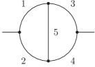
Figure 1: A two-loop propagator diagram

The subgraphs $\{1,2,5\}$ and $\{1,2,3,4\}$ are 1VI. The subgraph $\{1,2,3,5\}$ is 1VR and its 1VI components are $\{1,2,5\}$ and $\{3\}$. The subgraph $\{1,2,3\}$ is 1VR and its 1VI components are $\{1\}$, $\{2\}$ and $\{3\}$.

A set $f$ of 1VI subgraphs is called an ultraviolet (UV) forest if the following conditions hold:

(i) for any pair $\gamma,\gamma^{\prime}\in f$, we have either $\gamma\subset\gamma^{\prime}$, $\gamma^{\prime}\subset\gamma$ or ${\cal L}(\gamma\cap\gamma^{\prime})=\emptyset$;
(ii) if $\gamma^{1},\ldots,\gamma^{n}\in f$ and ${\cal L}(\gamma^{i}\cap\gamma^{j})=\emptyset$ for any pair from this family, the subgraph $\cup_{i}\gamma^{i}$ is 1VR.

In other words, the number of loops in $\cup_{i}\gamma^{i}$ (where $\gamma^{i}$ are disjoint with respect to lines and belong to a UV forest) is equal to the sum of the numbers of loops of $\gamma^{i}$. The term “UV” is used because the UV divergences are due to the integration over small values of $\alpha_{l}$ where the exponent in (1) is irrelevant and they are generated by the singularities of the factor ${\cal U}^{-d/2}$. We are going to show that the resolution of the UV singularities can be performed by the use of sectors associated with 1VI subgraphs.

For example, the set $\{1\}$, $\{2\}$, $\{3\}$ of subgraphs of Fig. 1 is a UV forest and $\{1,2,5\}$, $\{3\}$ is also a UV forest but the set $\{1\}$, $\{2\}$, $\{3\}$, $\{4\}$ is not a UV forest because the condition (ii) breaks down.

Let ${\cal F}$ be a maximal UV forest (i.e. there are no UV forests that include ${\cal F}$) of a given graph $\Gamma$. An element $\gamma\in{\cal F}$ is called trivial if it consists of a single line and is not a loop line. Any maximal UV forest has $h$ non-trivial and $L-h$ trivial elements.

Let us define the mapping $\sigma:\;{\cal F}\rightarrow{\cal L}$ such that $\sigma(\gamma)\in{\cal L}(\gamma)$ and $\sigma(\gamma)\not\!\,\in{\cal L}(\gamma^{\prime})$ for any $\gamma^{\prime}\subset\gamma$, $\gamma^{\prime}\in{\cal F}$. The inverse mapping $\sigma^{-1}:\;{\cal L}\rightarrow{\cal F}$ exists and can be defined as follows: $\sigma^{-1}(l)$ is the minimal element of the UV forest ${\cal F}$ that contains the line $l$. Let us denote by $\gamma_{+}$ the minimal element of ${\cal F}$ that strictly includes the given element $\gamma$.

For a given maximal UV forest ${\cal F}$, let us define the corresponding sector ($f$-sector) as

$${\cal D}_{\cal F}=\left\{\underline{\alpha}|\alpha_{l}\leq\alpha_{\sigma(\gamma)},\;l\in\gamma\in{\cal F}\right\}\;.$$ (5)

The intersection of two different $f$-sectors is of measure zero; the union of all the sectors gives the whole integration domain of the alpha parameters. For a given $f$-sector, let us introduce new variables labelled by the elements of ${\cal F}$,

$$\alpha_{l}=\prod_{\gamma\in{\cal F}:\;l\in\gamma}t_{\gamma}\;,$$ (6)

where the corresponding Jacobian is $\prod_{\gamma}t_{\gamma}^{L(\gamma)-1}$. The inverse formula is

$$t_{\gamma}=\left\{\begin{array}[]{ll}\alpha_{\sigma(\gamma)}/\alpha_{\sigma(\gamma_{+})}&\;\;\mbox{if $\gamma$ is not maximal}\\ \alpha_{\sigma(\gamma)}&\;\;\mbox{if $\gamma$ is maximal }\end{array}\right.\;.$$ (7)

Consider, for example, the following maximal UV forest ${\cal F}$ of Fig. 1 consisting of $\gamma^{1}=\{1\},\;\gamma^{2}=\{2\},\;\gamma^{3}=\{3\},\;\gamma^{4}=\{1,2,5\},\;\gamma^{5}=\Gamma$. The mapping $\sigma$ is $\sigma(\gamma^{1})=1,\;\sigma(\gamma^{2})=2,\;\sigma(\gamma^{3})=3,\;\sigma(\gamma^{4})=5,\;\sigma(\gamma^{5})=4$. The sector associated with this maximal UV forest is given by ${\cal D}_{\cal F}=\{\alpha_{1,2}\leq\alpha_{5}\leq\alpha_{4},\;\alpha_{3}\leq\alpha_{4}\}$ and the sector variables are $t_{\gamma^{1}}=\alpha_{1}/\alpha_{5},\;t_{\gamma^{2}}=\alpha_{2}/\alpha_{5},\;t_{\gamma^{3}}=\alpha_{3}/\alpha_{4},\;t_{\gamma^{4}}=\alpha_{5}/\alpha_{4},\;t_{\gamma^{5}}=\alpha_{4}$.

All the maximal UV forests of the given graph can be constructed at least in two ways.

Way 1. We imply that the lines are enumerated. Let us consider the sequence of subgraphs $\gamma_{l}$ consisting of lines $\{1,2,\ldots,l\}$, respectively, with $l=1,\ldots,L$. For each $l$, let us take the 1VI component of $\gamma_{l}$ that includes the line $l$. The set of all these components is a maximal UV forest. Then we construct in a similar way the UV forests for other $L!-1$ enumerations of the set of lines. After this we leave only distinct maximal UV forests.

Way 2. Since we consider a 1VI graph we include it into any maximal forest. Let us delete a line from it. The resulting graph is decomposed as the union of its 1VI components which we include into the maximal UV forest. Then we continue this process by deleting a line from some 1VI component which is not a single line, etc.

In the sector corresponding to a given maximal UV forest $f$, the function ${\cal U}$ takes the form

$${\cal U}=\prod_{\gamma\in f}t_{\gamma}^{h(\gamma)}\left[1+P_{f}\right]\;,$$ (8)

where $P_{f}$ is a non-negative polynomial and the product is over elements of the given maximal UV forest $f$. We will call such a factorization proper.

This factorization formula is proved by constructing an appropriate tree. One uses the relation

$$\prod_{l\not\!\,\in T}\alpha_{l}=\prod_{\gamma\in f}t_{\gamma}^{h(\gamma)+c(\gamma\cap T)-c(\gamma)}\;,$$ (9)

where $T$ is a tree or a 2-tree so that the factorization reduces to constructing a tree that provides the minimal value of the non-negative quantity $c(\gamma\cap T)-c(\gamma)$. Let $T_{0}$ be the tree composed of all trivial elements of the given maximal UV-forest $F$. In other words, this tree can be constructed as follows. One uses an order of lines which was used within Way 1 for the construction of the given maximal UV forest $f$ and includes the given line in the tree if a loop is not generated. One can obseve that this tree $T_{0}$ provides the zero value of $c(\gamma\cap T_{0})-c(\gamma)$ for all the elements of the given maximal forest.

To analyze convergence of the integral (1) large values of $\alpha_{l}$ (in particular, to reveal infrared (IR) divergences) one has to take into account the exponent as well. A possible way is to separate the integration over every $\alpha_{l}$ into $(0,1)$ and $(1,\infty)$ and then to deal with each of these $2^{L}$ regions separately — see, e.g. [10, 11]. This can be enough for a general analysis but cannot be good from the practical point of view because the number of the resulting sectors will be too large. A more reasonable approach is to turn [5] to an integral with a compact integration domain, where both UV and IR divergences are somehow mixed up and manifest themselves as divergences at small values of parameters of integration. We will do this in the next section.

3 Strategies to reproduce Hepp and Speer sectors

In [14], the starting point is the alpha representation (4) where primary sectors are introduced. The set of primary sectors corresponds to the different choices of a line in the given graph. At this step, one chooses a line $l=1,...,L$ and defines a sector $\Delta_{l}$ by $\alpha_{i}\leq\alpha_{l},\;i\neq l$ and the sector variables by $\alpha_{i}=t_{i}\alpha_{l},\;i\neq l$. The integration over $\alpha_{l}$ is then taken due to the delta function whose argument is supposed to be the sum of all the variables minus one.

One can also start directly from (1) and introduce primary sectors $\alpha_{i}\leq\alpha_{l},\;i\neq l$ there. For example, in the case of $l=L$, using the homogeneity properties of the functions in the representation and explicitly integrating over $\alpha_{L}$ we obtain the contribution of $\Delta_{L}$ as

$$F^{(L)} = \frac{\left(i\pi^{d/2}\right)^{h}\Gamma(a-hd/2)}{\prod_{l}\Gamma(a_{l})}\int_{0}^{1}\ldots\int_{0}^{1}\prod_{l}^{L-1}\alpha_{l}^{a_{l}-1}\,$$ (10)

$$\times\frac{\hat{\cal U}^{a-(h+1)d/2}}{\left[-\hat{\cal V}+\hat{\cal U}\left(\sum_{l=1}^{L-1}m^{2}_{l}\prod_{l=l^{\prime}}^{L-1}\alpha_{l^{\prime}}+m^{2}_{L}\right)\right]^{a-hd/2}}\mbox{d}\alpha_{1}\ldots\mbox{d}\alpha_{L-1}\;,$$

where

$$\hat{\cal U}={\cal U}(\alpha_{1},\ldots,\alpha_{L-1},1)\;,\;\;\;\hat{\cal V}={\cal V}(\alpha_{1},\ldots,\alpha_{L-1},1)\;.$$ (11)

Without loss of generality let us consider only this primary sector.

Let us remind that, for the case of non-zero masses, a general analysis of the factorization is not known even for Euclidean external momenta. Let us therefore turn to the pure massless case, as in [5]. Let us describe how sectors of Speer type can be introduced in such a way that the whole integrand of (10) has a proper factorization. As we could see in the previous section, the use of $f$-sectors provides a proper factorization (8) of the function $\cal U$ so that the factor $\hat{\cal U}^{a-(h+1)d/2}$ in (10) is properly factorized. However, these sectors generally do not provide a factorization of the second non-trivial factor. This can be seen using our example of Fig. 1. We are going to use smaller sectors which are in fact obtained from the $f$-sectors generated by the graph $\Gamma$ by a further decomposition.

Let $\Gamma^{\infty}$ be the graph obtained from $\Gamma$ by adding a new vertex $v^{\infty}$ and connecting it with all the external $n+1$ vertices by additional lines. These lines are only auxiliary and no propagators correspond to them. When writing down the function $\cal U$ for $\Gamma^{\infty}$, let us include, by definition, these additional lines into any tree. Then in the case of two external vertices (i.e. for $n=1$) we have

$${\cal V}_{\Gamma}={\cal U}_{\Gamma^{\infty}}q^{2}$$

where $q$ is the only external momentum.

Let us define sectors in a way similar to the previous section but using, instead of 1VI subgraphs, another set of subgraphs which we call $s$-irreducible. If a subgraph $\gamma$ does not have all the external vertices in the same connectivity component and if it is 1VI let us call it $s$-irreducible as well. If a subgraph $\gamma$ has all the external vertices in the same connectivity component let us call it $s$-irreducible if the graph $\gamma^{\infty}$ is 1VI. Then the maximal forests consisting of $s$-irreducible subgraphs can be constructed again by Way 1 or Way 2.

We define sectors (we name them Speer sectors) in a way similar to the sectors discussed in the previous section. We introduce sector variables by the same formula (6) as above. The factorization of the function $\cal V$ follows from its definition (3) and the auxiliary relation (9). The 2-tree that provides a minimal value of the non-negative quantity $c(\gamma\cap T)-c(\gamma)$ can be constructed by a procedure similar to the procedure used for the function $U$: one considers the lines in the order used for the construction of the given $f$-forest by Way 1 and includes the given line into the 2-tree if a loop is not generated and if this is not the line whose inclusion would connect all the external vertices.

By construction, for such a 2-tree $T_{0}$, we obtain $c(\gamma\cap T_{0})-c(\gamma)=\theta(\gamma)$ where $\theta(\gamma)=1$ if the external vertices are connected in $\gamma$ and $\theta(\gamma)=0$ otherwise. Hence we obtain a proper factorization

$${\cal V}=\prod_{\gamma\in f}t_{\gamma}^{h(\gamma)+\theta(\gamma)}\left[q^{2}_{T_{0}}+P_{\cal V}\right]\;,$$ (12)

where $P_{\cal V}$ is a non-negative polynomial.

Obviously, the Speer sectors can be obtained from those associated with the graph $\Gamma$ by a further decomposition, so that the factorization of the function ${\cal U}$ in the corresponding variables also holds and has the form similar to (8) with the same exponents.

Let us turn to the modern strategies of sector decompositions. After introducing primary sectors, one obtains the contribution (10) and other $L-1$ contributions of the same type. At each step, one chooses a subset of the indices $\nu=\{i_{1},\ldots,i_{k}\}$ and an index $i_{r}$ from this subset and defines a sector $\alpha_{i}\leq\alpha_{i_{r}},\;i\neq i_{r}$ and the sector variables by $\alpha_{i}=t_{i}\alpha_{i_{r}},\;i\neq i_{r}$ To formulate a strategy of introducing iterative sectors one needs to fix rules for determining subsets $\nu$ at every recursive step .

The first know sector decomposition strategy is described in [14]; three strategies guaranteed to terminate ($A$, $B$ and $C$) and one strategy not guaranteed to terminate ($X$) are presented in [19]; they all are based on analyzing the functions $\cal U$ and $\cal V$ and choosing a subset of indices depending on their properties. Strategy $S$ [20] is a bit different and is based on analyzing the polytopes of weights and their lowest faces.

With the Hepp sectors, the situation is obvious: they are reproduced when we consider maximal subsets of lines at each step, i.e. with one line less than before this.

To reproduce the choice of Speer sectors within a sector decomposition let us remind the Way 2 to construct sectors. One has to consider only subsets of the indices $\nu=\{i_{1},\ldots,i_{k}\}$ that correspond to $s$-irreducible subgraphs.

We compared the number of sectors for numerous examples and discovered a curious phenomenon: the set of the sectors within Strategy S and the set of the Speer sectors is always the same. In particular, this is observed in the two examples of massless vertex diagrams shown in Fig. 2 at Euclidean external momenta,

Figure 2: Vertex off-shell diagrams

and in rather non-trivial examples of three four-loop propagators diagrams of Fig. 3

Figure 3: Most complicated four-loop propagator diagrams

which are the most complicated master integrals among all four-loop massless propagators integrals.

diagram	S	X
v2	102	102
v3	2160	2251
m61	26208	32620
m62	26304	27540
m63	27336	failed

The results of this analysis are shown in Table 1 where the number of the sectors is shown. The first column stands for Strategy S and Speer sectors; the resulting number of the sectors is the same. For comparison, we included the second column for Strategy X [19] which has been proved to be very effective in a number of complicated calculations. Here ‘failed’ means that a factorization by sector decomposition has not been achieved for a reasonable amount of time (at least not for one day.)

4 Conclusion

In fact, our motivation to recall Speer sectors was to suggest to use them within FIESTA since they are optimal for Feynman integrals at all Euclidean external momenta. However it turned out that these sectors are reproduced, in rather nontrivial examples, within Strategy S. Therefore we can conclude that Strategy S has chances to be an optimal universal strategy which always terminates and provides a proper factorization.

Let us remind that Speer sectors have a certain physical meaning: the integration over the sector variable $t_{\gamma}$ is responsible for UV divergences and, if $\gamma$ contains all the external vertices, for off-shell IR divergences. If on-shell and collinear divergences are present, Speer sectors are no longer applicable. Then one can use sector decompositions, e.g. within Strategy S, and this strategy could help to reveal the physical meaning of the sectors. To do this one might start with analyzing simple typical diagrams with on-shell or/and collinear divergences.

Acknowledgments. We are grateful to G. Heinrich for helpful discussions. Many thanks to N. Glover for kind hospitality during our visit to the Institute of Particle Physics Phenomenology in Durham, where a part of this work was done. The work was supported by the Russian Foundation for Basic Research through grant 08-02-01451.

References

- [1] N.N. Bogoliubov and D.V. Shirkov, Introduction to theory of quantized fields, 3rd edition, Wiley, New York (1983).
- [2] N. Nakanishi, Graph theory and Feynman integrals, Gordon and Breach, New York (1971).
- [3] K. Hepp, Proof of the Bogolyubov-Parasiuk theorem on renormalization, Commun. Math. Phys. 2 (1966) 301.
- [4] E.R. Speer, Analytic renormalization, J. Math. Phys., 9 (1968) 1404.
- [5] E.R. Speer, Ultraviolet and infrared singularity structure of generic Feynman amplitudes, Ann. Inst. H. Poincaré, 23 (1977) 1.
-
[6]
M.C. Bergère and J.B. Zuber,
Renormalization of Feynman amplitudes and parametric integral
representation,
Commun. Math. Phys. 35 (1974) 113;
M.C. Bergère and Y.M. Lam, Bogolyubov–Parasiuk theorem in the alpha parametric representation, J. Math. Phys. 17 (1976) 1546. - [7] M.C. Bergère, C. de Calan and A.P.C. Malbouisson, A theorem on asymptotic expansion of Feynman amplitudes, Commun. Math. Phys. 62 (1978) 137.
- [8] P. Breitenlohner and D. Maison, Dimensional renormalization and the action principle, Commun. Math. Phys. 52 (1977) 11; Dimensionally renormalized Green’s functions for theories with massless particles, Commun. Math. Phys., 52 (1977) 39, 55.
- [9] K. Pohlmeyer, Large momentum behavior of the Feynman amplitudes in the in four-dimensions theory, J. Math. Phys. 23 (1982) 2511.
-
[10]
O.I. Zavialov, Renormalized quantum field theory, Kluwer Academic Publishers,
Dodrecht (1990);
V.A. Smirnov, Asymptotic expansions in limits of large momenta and masses, Commun. Math. Phys. 134 (1990) 109. - [11] V.A. Smirnov, Applied asymptotic expansions in momenta and masses, STMP 177, Springer, Berlin, Heidelberg (2002).
- [12] G. ’t Hooft and M. Veltman, Regularization and renormalization of gauge fields, Nucl. Phys. B 44 (1972) 189.
- [13] C.G. Bollini and J.J. Giambiagi, Dimensional renormalization: the number of dimensions as a regularizing parameter, Nuovo Cim. B 12 (1972) 20.
- [14] T. Binoth and G. Heinrich, An automatized algorithm to compute infrared divergent multi-loop integrals, Nucl. Phys. B 585 (2000) 741 [arXiv:hep-ph/0004013]; Numerical evaluation of multi-loop integrals by sector decomposition, Nucl. Phys. B 680 (2004) 375 [arXiv:hep-ph/0305234]; Numerical evaluation of phase space integrals by sector decomposition, Nucl. Phys. B 693 (2004) 134 [arXiv:hep-ph/0402265].
- [15] G. Heinrich, Sector decomposition, Int. J. Mod. Phys. A 23 (2008) 1457 [arXiv:0803.4177 [hep-ph]].
- [16] V.A. Smirnov, Analytical result for dimensionally regularized massless on-shell planar triple box, Phys. Lett. B 567 (2003) 193 [arXiv:hep-ph/0305142].
-
[17]
T. Gehrmann, G. Heinrich, T. Huber and C. Studerus,
Master integrals for massless three-loop form factors: one-loop and
two-loop insertions,
Phys. Lett. B 640 (2006) 252
[arXiv:hep-ph/0607185];
G. Heinrich, T. Huber and D. Maitre, Master integrals for fermionic contributions to massless three-loop form factors, Phys. Lett. B 662 (2008) 344 [arXiv:0711.3590 [hep-ph]]. - [18] R. Boughezal and M. Czakon, Single scale tadpoles and O(G(F) m(t)**2 alpha(s)**3) corrections to the rho parameter, Nucl. Phys. B 755 (2006) 221 [arXiv:hep-ph/0606232].
- [19] C. Bogner and S. Weinzierl, Resolution of singularities for multi-loop integrals, Comput. Phys. Commun. 178 (2008) 596 [arXiv:0709.4092 [hep-ph]]; Blowing up Feynman integrals, Nucl. Phys. Proc. Suppl. 183 (2008) 256 [arXiv:0806.4307 [hep-ph]].
- [20] A.V. Smirnov and M.N. Tentyukov, Feynman Integral Evaluation by a Sector decomposiTion Approach (FIESTA), arXiv:0807.4129 [hep-ph].
-
[21]
V.N. Velizhanin,
Leading transcedentality contributions to the four-loop universal anomalous
dimension in SYM,
arXiv:0811.0607 [hep-th];
G. Bell, NNLO corrections to inclusive semileptonic B decays in the shape-function region, arXiv:0810.5695 [hep-ph];
Y. Kiyo, D. Seidel and M. Steinhauser, corrections to the vertex at the top quark threshold, arXiv:0810.1597 [hep-ph];
R. Bonciani and A. Ferroglia, Two-loop QCD corrections to the heavy-to-light quark decay, arXiv:0809.4687 [hep-ph];
A.V. Smirnov, V.A. Smirnov and M. Steinhauser, Fermionic contributions to the three-loop static potential, Phys. Lett. B 668 (2008) 293 [arXiv:0809.1927 [hep-ph]]. - [22] P.A. Baikov and K.G. Chetyrkin, in preparation.