Modeling tumor cell migration: From microscopic to macroscopic models

Abstract

It has been shown experimentally that contact interactions may influence the migration of cancer cells. Previous works have modelized this thanks to stochastic, discrete models (cellular automata) at the cell level. However, for the study of the growth of real-size tumors with several million cells, it is best to use a macroscopic model having the form of a partial differential equation (PDE) for the density of cells. The difficulty is to predict the effect, at the macroscopic scale, of contact interactions that take place at the microscopic scale. To address this, we use a multiscale approach: starting from a very simple, yet experimentally validated, microscopic model of migration with contact interactions, we derive a macroscopic model. We show that a diffusion equation arises, as is often postulated in the field of glioma modeling, but it is nonlinear because of the interactions. We give the explicit dependence of diffusivity on the cell density and on a parameter governing cell-cell interactions. We discuss in detail the conditions of validity of the approximations used in the derivation, and we compare analytic results from our PDE to numerical simulations and to some in vitro experiments. We notice that the family of microscopic models we started from includes as special cases some kinetically constrained models that were introduced for the study of the physics of glasses, supercooled liquids, and jamming systems.

I Introduction

The migration of tumor cells plays a principal role in tumor malignancy, particularly for brain tumors. The fact that glioma cells migrate fast contributes greatly to glioblastoma lethality and thwarts therapy strategies based on tumor resection Giese et al. (2003). Understanding the mechanisms of migration can be of utmost importance when it comes to devising efficient treatments Demuth and Berens (2004); Nakada et al. (2007). In vitro studies combined with mathematical models constitute a promising exploration path, a fact supported by several high-quality results Frieboes et al. (2006); Stein et al. (2007).

How does one go about modeling cell migration? There are essentially two approaches: on one hand, “macroscopic” models that take the mathematical form of one or several partial differential equations (PDE) Murray (2002a); Bellomo et al. (2008), and, on the other hand, “microscopic” models where individual cells are represented and evolve according to some (stochastic) rules: the so-called individual based models, agent based models, cellular automata, and so on Alber et al. (2003); Deutsch and Dormann (2005); Hatzikirou and Deutsch (2008); Anderson et al. (2007).

In a macroscopic model, one eschews all reference to the elementary constituent, the cell, and introduces macroscopic quantities, like the average cell density, which evolve according to a PDE. One expects stochastic deviations from the average to be negligible at the scale of a large population of cells, provided this population is homogeneous (quite often, cell populations in cancer are made of cells having distinct phenotypes or genotypes, because e.g., of genetic mutations Nowell (2002); Weinberg (2007); Bellomo and Delitala (2008), and this should be taken into account in a more general model of cancer development). As a matter of fact, the first brain tumor models (and the vast majority of models existing today, which are essentially refinements of these first ones) consider the dynamics of a small number of macroscopic quantities Tracqui et al. (1995); Tracqui (1995); Woodward et al. (1996). The tumor cell density is, of course, incontrovertible, the remaining quantities being usually concentrations of chemicals, which, one surmises, play a role in the migration.

Using a PDE has many advantages over a “microscopic” model. First, even with the ultrasimplification of a cellular automaton, one can treat a relatively small number of cells, at best a few thousand, a number very far from the millions one encounters in a tumor lump. Then, there are ready-to-use PDE solvers. Since the PDEs are deterministic, one simulation is enough where one should perform many simulations of the cellular automaton to average over the stochastic noise. The number of discretization steps of the space is fixed only by the mesoscopic geometry of the medium in which the cells diffuse; there is no need to have as many steps as cells. Finally, it is easier to get analytical results from a PDE (even approximate) than from a cellular automaton.

In this spirit, the simplest approach to cell migration is to assimilate the process to linear diffusion. Then a diffusion equation may be used to find how the cell density evolves with time,

$$\frac{\partial\rho}{\partial t}=D\,\nabla^{2}\rho.$$ (1)

This was, for instance, the approach of Burgess et al. Burgess et al. (1997), who modeled the evolution of glioblastomas with the help of a diffusion equation (plus an exponential growth representing cell proliferation). Refinements of the diffusion model can be, and have been, introduced. One can, for instance, consider a space-dependent diffusion coefficient that varies depending on the nature of the tissue in which migration takes place Swanson et al. (2000, 2003); Jbabdi et al. (2005); Clatz et al. (2005). Terms can be added to Eq. (1) representing various chemotactic effects, either as arbitrary external source terms or as quantities that couple Eq. (1) to other evolution equations Sander and Deisboeck (2002); Castro et al. (2005). When the cells have a velocity or a persistence of the direction of motion, one has to study (e.g., at short time scales of the cell migration) a different type of equation, like a hyperbolic PDE or a degenerate parabolic PDE Othmer and Hillen (2002); Filbet et al. (2005); Dolak and Schmeiser (2005); Bellomo et al. (2007).

However, modeling of cell migration as simple, heatlike diffusion (noninteracting random walks Othmer et al. (1988); Codling et al. (2008)) neglects important phenomena, even in the absence of chemotaxis: cells cannot penetrate each other, and they often interact via contacts with other cells and/or with the extracellular matrix.

But what PDE should one use to take contact interactions into account in the migration process? It can be easier to devise realistic evolution and interaction rules in a cell-based model Schaller and Meyer-Hermann (2006); Hatzikirou and Deutsch (2008); Anderson et al. (2007). Even though there are situations in which it is not possible to discriminate between several macroscopic models, especially when only data for the evolution of the cell density are at hand Simpson et al. (2007); Schaller and Meyer-Hermann (2006); Cai et al. (2006), it is of little interest to use a PDE that can later prove to be wrong when more data become available and, in particular, when one is able to compare predictions for the trajectories of individual cells Simpson et al. (2007); Schaller and Meyer-Hermann (2006); Stein et al. (2007).

Sometimes, a microscopic model is derived from a PDE through a discretization procedure Anderson and Chaplain (1998). But there are several ways to discretize space that lead to very different behavior of the microscopic agents, some of which can be unrealistic. (For example, consider the discretized population pressure model of Cai et al. (2006): one can show that, for some discretization procedure, cells move toward the high-density region they are supposed to flee, but for some other procedure they move away from it — and both correspond to the very same PDE.) At least, one needs a biological criterion to choose the “right” discretized version of the PDE.

Therefore, to establish a macroscopic model for tumor cell migration with contact interactions via the so-called gap junctions between cells, we start from the microscopic model introduced and successfully compared to in vitro migration experiments in Aubert et al. (2006). In this setting, cell proliferation, apoptosis (cell death), and mutations (changes of cell behavior) are negligible (hence the population is homogeneous). The number of cells is constant and cells simply move on a collagen substrate. The model is defined in Sec. II. (There we also discuss special cases in which our model is a kinetically constrained model, borrowing some knowledge from the theory of glasses, supercooled liquids, and jamming systems.)

The derivation of the macroscopic model, the so-called hydrodynamic limit, is carefully explained in Sec. III. The derivation of hydrodynamic limits is a well-known technique in mathematical physics Lebowitz et al. (1988); Spohn (1991); De Masi and Presutti (1991); Kipnis and Landim (1999); Deutsch and Lawniczak (1999), and it has also been used in mathematical biology Bellomo et al. (2008); Othmer and Hillen (2002); Filbet et al. (2005); Dolak and Schmeiser (2005); Bellomo et al. (2007). See Turner et al. (2004); Drasdo (2005); Alber et al. (2006); Lushnikov et al. (2008) for examples in the field of cell movement and cancer modeling. Since our derivation relies on a mean-field like approximation, we review in Sec. III the circumstances under which the approximation fails, and we provide thorough comparisons to simulation results.

The PDE we obtain is a nonlinear diffusion equation. Contrary to what is customary in the phenomenological models to which we alluded above, the terms of the diffusion equation depend crucially on the cell-cell interaction present in the microscopic model. As our analysis shows, these interactions introduce nonlinearities in the diffusion equation. These nonlinearities are essential in order to reproduce the density profiles obtained in in vitro migration experiments (Sec. IV).

II The stochastic cellular automaton model

In Aubert et al. (2006), a cellular automaton (lattice gas) was introduced to mimic the migration of cancer cells with contact interactions. The dynamics of migratory motion are described through the evolution of points (representing the cells) on a grid (or lattice), while the interactions are introduced through evolution rules. The impossibility of cells to penetrate each other is trivially taken into account (no two cells can share the same position on the grid), and the scale length of the lattice step is the typical size of one cell.

It is easy to extend such a cellular automaton to cells that occupy several sites on the lattice, using e.g., a cellular Potts model  Turner et al. (2004); Alber et al. (2006); Anderson et al. (2007); Lushnikov et al. (2008). But then we would need to introduce many parameters (surface tension, binding energies, …), whereas experimental data at hand were not sufficient to measure so many values and avoid dubious fits. Thus the model of Aubert et al. (2006) is an elementary cellular automaton with nonextended cells, involving a single parameter that takes contact interactions into account. This approach has made it possible to model with success the migration of glioma cells over substrates of collagen or of astrocytes and draw conclusions on the existence of homotype and heterotype interactions between the cells Aubert et al. (2006, 2008).

In order to define a cellular automaton model, one needs two things. First, one must choose the geometry of the lattice. One may work in one, two, or three dimensions and consider elementary cells of any shape and size. Second, one must specify the update rules of the automaton. With the adequate choice of these rules, one can mimic the interactions between the elementary entities (glioma cells in Aubert et al. (2006)) which are modeled by the automaton. In this paper, we shall follow the prescriptions we introduced in Aubert et al. (2006). We recall them briefly below.

II.1 The geometry

The cellular automaton introduced in Aubert et al. (2006) for the description of the glioma cell migration is based upon a regular hexagonal tiling (or, equivalently, a triangular lattice). This choice is dictated by the fact that the hexagonal tiling is the less anisotropic among all regular tilings of the plane. Thus one can have a very simple algorithmic definition of the geometry while keeping the constraints due to the symmetry of the lattice at a minimum. Moreover, in such a lattice each cell is surrounded by six sites, a number sufficiently high to allow a certain freedom of motion at each update. A generalization to three space dimensions is obtained by considering the face-centered-cubic (fcc) lattice or the hexagonal compact (hc) lattice, where each site has 12 nearest)-neighbor sites. It is known that some difficulties arise in three-dimensional lattices as compared to two-dimensional lattices when one aims at finding a cellular automaton, the continuous limit of which would be the Navier-Stokes equation Frisch et al. (1986); d’Humières et al. (1986), but here we have no such constraint: instead of starting from a macroscopic equation (such as the Navier-Stokes equation) and guessing what cellular automaton would mimick it, we start from a given cellular automaton and ask for (an approximation to) the corresponding macroscopic equation. The only constraint is that the macroscopic equation be a reasonable model of the behavior of real cells in experiments. Additionally, it turns out that both the fcc and hc lattices, although they do not have the same symmetry properties , lead to the same macroscopic equation. Therefore, we expect that refinements in the choice of the three-dimensional lattice would not significantly change our results.

In each case, we denote by $a$ the distance between the centers of two nearest-neighbor sites (lattice step).

II.2 The stochastic evolution rules

Each hexagon can be occupied by at most one cell at a time. As a consequence, a cell can move only to a free site. The total number of cells is locally conserved (but cells may be introduced into or removed from the system on the boundaries). Thus our automaton is a kind of lattice gas or “box and ball” system Takahashi and Matsukidaira (1997). Notice that our model is not a so-called lattice-gas cellular automaton (LGCA), where individual particles have both a position and a speed: here the cells lose the memory of their speed and previous position after each move. In the classification of Othmer et al. (1988), it is a “position jump process,” not a “velocity jump process.”

At each update of the automaton (discrete time step), the process of picking a lattice site at random and applying the stochastic evolution rules to this site is repeated a number of times equal to the total number of sites, so that, on average, each site is updated once at each time step . If the site is empty, nothing happens. If it is occupied by one cell, the following rule is applied. It is inspired by what we believe is the biological mechanism of contact interaction. The interaction paremeter $p$ is a fixed, constant number between 0 and 1. We pick at random one of the six neighboring sites, the target site. If the target site is occupied, nothing happens. Otherwise, the move from the cell to the target site (leaving its departure site empty) is done with probability $p$ if at least one of the two common neighboring sites of the departure site and of the target site is occupied, and with probability $1-p$ if the two common neighboring sites are empty. With these assumptions, $p=1$ means that a cell can only move if it is in close contact with at least one other cell, and it can only move to a position where it will stay in contact with a least one of its former neighbors, while, for $p=0$, a cell moves only in such a way that all contacts to its former neighbors are broken. If $p=\frac{1}{2}$, cells are indifferent to their environment (apart from mutual exclusion), and we expect that the cell density obeys a diffusion equation. Values of $p>\frac{1}{2}$ model situations in which cells are reluctant to break established junctions with their neighbors, whereas $p<\frac{1}{2}$ involves a kind of short-range repulsion but only between cells that were in close contact, unlike what is usually called repulsion between, e.g., electric charges. If these rules seem odd from a physical point of view (they cannot be related to some energy or free energy and convey a strange notion of repulsion, and in particular they do not reduce to a special case of the model of Lushnikov et al. (2008)), they incorporate the biologically reasonable assumption that a cell makes its decision regarding where it goes by considering only information it can get from its immediate vicinity, e.g., through established communication junctions with the cells with which it is in contact.

The preceding rules can readily be extended to the three-dimensional hexagonal compact or fcc lattices; the only change is that a pair of a departure and a target site has four neighbors in common instead of two.

The setting considered in Aubert et al. (2006) consists in a central part of the lattice occupied by the equivalent of the glioma cell spheroid, which, we assumed, acts as a cell source. Once a free position in the hexagons surrounding the center appears, it is immediately occupied by a cell “released from the center.” In Aubert et al. (2006), we have explained how one can (and must) calibrate the model so as to allow quantitative comparisons with experiment.

II.3 Kinetically constrained models

Our cellular automaton contains as special cases (for $p=1$ and 0) two kinetically constrained models (KCMs). These models were introduced in statistical physics to mimic the dynamics of glasses, supercooled liquids, and jamming systems Ritort and Sollich (2003); Toninelli and Biroli (2007).

In a KCM, a microscopic object (in our context, cells) can move to a free position only if some requirement about its neighborhood is fullfilled (e.g., only if it has at least another empty position around itself). As a consequence, at least for some concentrations of surrounding cells, the motion of an individual cell is not a Brownian motion, as it is in a diffusive model such as the simple symmetric exclusion processes ($p$ close to $\frac{1}{2}$). However, if one does a “zoom out” or coarse-graining of the trajectory of an individual cell, using characteristic length and time scales (which depend on the concentration of cells) as new unit length and time, the result looks Brownian Berthier et al. (2005). Above these scales, a diffusion equation should hold.

The origin of this separation of scales and the existence of the characteristic length and time scales is easy to understand for the so-called noncooperative KCMs (modeling strong glass-former materials). There, cells are blocked unless they are close to some model-dependent defect or excitation that has a finite size. These excitations travel across the system in a kind of diffusive motion, and the configuration of the cells in a region will be changed or relaxed only after the region has been traversed by an excitation. Even though the excitations, and the individual cells while they are close to an excitation, diffuse “quickly,” a cell goes “slowly” away from its initial position because its trajectory is an alternation of long nonmoving phases (when the cell is away from any excitation) and short diffusive phases (when the cell is close to an excitation) Jung et al. (2004); Berthier et al. (2005). The characteristic time scale is the typical time between two stays of an excitation in the neighborhood of a cell, and the characteristic length is the typical size of the region explored by a cell during such a stay. Over times much greater than the characteristic time, the trajectory of a cell is made of many nearly independent non-moving/quickly diffusive patterns and, according to the central limit theorem, the cell undergoes a Brownian motion with an effective diffusion constant. Fick’s law is obeyed and the coarse-grained model is like a lattice gas without kinetic constraints Toninelli and Biroli (2007).

In the case of the cooperative KCMs (modeling fragile glass-formers), no traveling finite-size excitation facilitating the motion of cells exists. Instead, the moves of the cells are organized hierarchically and form structures that can be infinitely large Hedges and Garrahan (2007): some changes of the system require the participation of an extensive fraction of the cells, hence the term “cooperative”. A complete blocking at a finite concentration of cells can even be observed for some models Toninelli and Biroli (2007). Still, in the absence of such blocking, it is possible to define a characteristic time and a characteristic scale above which a diffusive behavior is recovered and Fick’s law is obeyed Pan et al. (2005).

In our cellular automaton, both the noncooperative and cooperative behaviors take place, for $p=1$ and 0, respectively (and the behavior for $p$ close to 0, on the one hand, and for $p$ close to 1, on the other, is qualitatively the same as in these two limit situations).

For $p=1$, our model is a noncooperative KCM: according to the rules of the automaton, an isolated cell cannot move, but a cluster of two neighboring cells has a finite probability to go anywhere in the lattice and it can be “used” to move any isolated cell (it plays the role of the aforementioned excitations).

For $p=0$, our model is a cooperative KCM: this is the very same model as the “2-triangular lattice gas” or (2)-TLG studied in the context of the slow dynamics of glasses Jäckle and Krönig (1994); Krönig and Jäckle (1994); Pan et al. (2005); Hedges and Garrahan (2007).

To conclude, for general $p$, our model interpolates between a cooperative KCM ($p=0$), a simple symmetric exclusion process ($p=\frac{1}{2}$) and a noncooperative KCM ($p=1$).

III The hydrodynamic limit

In this section, we explain in detail how we derive an approximate macroscopic, deterministic model (which takes the form of a partial differential equation) from the microscopic, stochastic cellular automaton. This kind of technique has been used in physics since the 1980s to take the so-called hydrodynamic limit of a stochastic model. We recall the basics for readers who are not familiar with it. Other readers may be interested in our discussion of rigorous results and of the quality and limits of our approximation.

The hydrodynamic limit exists for some model defined on a lattice if, as the size of the lattice goes to infinity, one can cut the lattice into parts such that (i) the parts are negligibly small with respect to the whole lattice, (ii) the values that macroscopic quantities (like the cell concentration) take for each part have vanishingly small fluctuations, and (iii) the averages of these values obey some partial differential equation(s). This process is a kind a coarse-graining. Similarly, water, though made of discrete molecules, looks like a fluid composed of homogeneous droplets, because each droplet contains a huge number of molecules that are typically spread homogeneously in the droplet rather than all packed in one-half of the droplet.

The establishment of a PDE for macroscopic quantities after coarse-graining has been extensively studied and can be made mathematically rigorous in a number of cases (see, e.g., Lebowitz et al. (1988); Spohn (1991); De Masi and Presutti (1991); Kipnis and Landim (1999)). We would like to show that, although one might think that this continuous time and continuous space approximation is useful only in the case of very large lattices, it yields results in excellent agreement with the results from our cellular automaton for lattices as small as 16$\times$16. Indeed, even if in one simulation (or in one experiment) the microscopic concentration of tumor cells is discrete (it can take only two values on each lattice site, depending on whether the site is full or empty), the average of this concentration over independent simulations of the cellular automaton (or over independent experiments) is well predicted by the PDE. Furthermore, there are many ways to perform the approximation, some of which being rather involved, but we show that, here, an elementary procedure that can easily be applied to other cellular automata is sufficient.

III.1 On the existence and scale of the validity of the hydrodynamic limit

Several authors have proven rigorously that some cellular automata have a nonlinear diffusion equation as their macroscopic scaling limit Fritz (1987); Guo et al. (1988); Varadhan (1991); Varadhan and Yau (1997). In particular, the theorem of Varadhan and Yau (1997) proves that our model has a hydrodynamic limit for all values of $p$ between 0 and 1 excluded (we have to exclude 0 and 1 because, for them, some transition rates are 0 and the theorem does not apply). However, it seems rather complicated to get an explicit formula for the corresponding nonlinear diffusion equation from this theorem. On the contrary, our computation provides approximate but explicit formulas that are very useful most of the time.

When $p=1$ or 0, one needs to be more careful: then, we have seen in Sec. II that the cellular automaton is a KCM where Fick’s law is obeyed only above some characteristic length and time scales.

Very recently, Gonçalves et al. constructed some KCM, the hydrodynamic limit of which would be the porous media equations, and they were able to prove this rigorously Gonçalves et al. (2007). For $p=1$, our model is only slightly different from theirs and we believe that generalizing their proof to ours would be possible. This is an indication that (nonlinear) diffusion should hold above some spatial scale, but in practice it is necessary to know how large this scale is. We found that, for $p=1$, and more generally for all values of $p$ not close to zero, this scale is of the order of the elementary lattice spacing — the agreement between simulations of the cellular automaton and solutions of the PDE is excellent already at this scale (see later).

For $p=0$, we know from the previous section that our model is a cooperative KCM (the “2-triangular lattice gas” Jäckle and Krönig (1994); Krönig and Jäckle (1994)). To the best of our knowledge, there is no rigorous proof of the hydrodynamic limit in this case or in a similar case, but it is highly probable that this limit exists because the length and time scales we have discussed above exist in particular for this model Pan et al. (2005) (they diverge as the cell concentration goes to 1, but are otherwise finite). We found that our approximation breaks down as $p$ gets close to 0, which is a sign that the kinetics cannot be understood only by looking at one cell and its nearest neighbors. Still, $p$ needs to be as small as 0.05 for one to see a significant discrepancy between our approximation and the automaton.

III.2 Formalism and computation

We now proceed with our computation. On the basis of the previous considerations, this approximate computation should be valid only if the spatial scale above which a macroscopic, coarse-grained diffusive behaviour is of the order of the lattice size — fortunately, this is the case for most values of $p$.

Our procedure involves first taking averages over the stochastic noise, neglecting correlations, in order to yield deterministic equations on the lattice, then taking the continuous space limit to go from the microscopic to the macroscopic scale. Of course, averaging over the noise amounts to losing information about the true process. Describing the behavior of a few cells on the lattice by the sole average of the cell concentration on each lattice site would be a crude approximation, of little interest. However, one can hope that this approximation is not so bad in the presence of a large number of cells, and that the typical fluctuations of interesting macroscopic quantities such as the cell concentration become very small as the system grows. Conversely, large fluctuations of the macroscopic quantities would become very rare as the system grows. As we shall see, this does happen for our model and the deterministic, continuous space aproximation is already excellent for rather small systems.

III.2.1 Averaging over the stochastic noise

To perform the averaging and neglect correlations, we use a technique that is similar to the Hubbard-Stratonovich transform and which was already used to study another cellular automaton, the contact process Deroulers and Monasson (2004). This technique may be used to build a perturbative expansion. Here, we will actually stop at the first order, since it yields results that are already in excellent agreement with our numerical simulations. Therefore, introducing the technique is not necessary and one can get the same results using other means. But we explain it because its formalism is convenient and compact, especially if one wants to use computer algebra to compute the macroscopic PDE on complicated or high-dimensional lattices. In addition, it yields access to systematic perturbative corrections (we can, in principle, get closer and closer to the exact result by keeping more and more terms) on one hand, and to large deviations properties, on the other hand (see Deroulers and Monasson (2004) for an example where large deviations properties are crucial).

Using the now standard “quantumlike” formalism for master equations, introduced a long time ago Kadanoff and Swift (1968); Felderhof (1971b, a); Doi (1976), we start by representing the probability distributions of the configurations of the cellular automaton as vectors in a simplex. The stochastic rules are encoded as a linear operator acting on this space.

For each site $i$ of the lattice, we introduce two basis vectors $|0_{i}\rangle$ and $|1_{i}\rangle$ to encode the situations in which the site is empty and occupied by one cell, respectively. If the lattice had only one site, say $i$, only two configurations would be possible (“the site is occupied by a cell” or “the site is empty”) and it would be enough to specify the occupation probability $\rho$ of the (unique) site to characterize entirely the statistical distribution of the configurations under some fixed environment. In our formalism, we represent this distribution by the vector $v_{i}:=\rho\,|1_{i}\rangle+(1-\rho)\,|0_{i}\rangle$; the coefficient of each basis vector is the probability of observing the corresponding configuration (there is no need to take the square modulus as in quantum mechanics). If the lattice is composed of two sites, say $i$ and $j$, there are four configurations and the most general probability distribution can be represented by the vector $\alpha\,|0_{i},0_{j}\rangle+\beta\,|0_{i},1_{j}\rangle+\gamma\,|1_{i},0_{j}\rangle+\delta\,|1_{i},1_{j}\rangle$ with $\alpha+\beta+\gamma+\delta=1$ (probabilities must sum up to 1). Here, the four basis vectors are the tensor products of the basis vectors for the site $i$ and of the site $j$: $|1_{i},0_{j}\rangle=|1_{i}\rangle\otimes|0_{j}\rangle$ and so on. In the special case in which the sites $i$ and $j$ are statistically independent (in which case the probability that $i$ is occupied and $j$ is occupied is the product of the occupation probabilities of $i$ and $j$, say $\rho_{i}$ and $\rho_{j}$, respectively), this vector factorizes as $[(1-\rho_{i})|0_{i}\rangle+\rho_{i}|1_{i}\rangle]\otimes[(1-\rho_{j})|0_{j}\rangle+\rho_{j}|1_{j}\rangle]$. More generally, if there are $N$ sites, there are $2^{N}$ possible configurations and our vector space has dimension $2^{N}$.

To explain how we encode the stochastic rules, let us take again the simple case in which the lattice has only one site. Let us address first the stochastic process of “radioactive decay”: when the site is full, it has a constant probability per unit time $\alpha$ to become an empty site, and, when it is empty, it remains so. The occupation probability $\rho_{i}(t)$ of the site obeys the differential equation

$$\mathrm{d}\rho_{i}/\mathrm{d}t=-\alpha\,\rho_{i}(t).$$ (2)

This equation is called the master equation or the Chapman-Kolmogorov equation. The vector that encodes the probability distribution, $v_{i}(t)$, obeys

$$\mathrm{d}v_{i}(t)/\mathrm{d}t=\alpha(c_{i}-c^{+}_{i}c_{i})v_{i}(t),$$ (3)

where $c_{i}$ and $c^{+}_{i}$ are $2\times 2$ matrices: in the basis $|0\rangle,|1\rangle$,

$$c_{i}=\left(\begin{array}[]{cc}0&1\\ 0&0\end{array}\right)\qquad\mathrm{and}\qquad c^{+}_{i}=\left(\begin{array}[]{cc}0&0\\ 1&0\end{array}\right).$$ (4)

The symbols for these matrices are borrowed from quantum mechanics, since $c$ and $c^{+}$ behave like annihilation and creation matrices, respectively (for so-called hardcore bosons). The evolution operator $c_{i}-c^{+}_{i}c_{i}$ of vector $v_{i}$ has two terms: the first one, $c_{i}$, lets the probability of the configuration $|0\rangle$ increase proportionnally to the probability of the configuration $|1\rangle$, and, without the second one, probability conservation would not be ensured because the probability of the configuration $|1\rangle$ would be unchanged. Let us give a second example in which two sites $i$ and $j$ are coupled: consider the stochastic process in which a particle is transferred from the site $i$ (if site $i$ is occupied) to the site $j$ (if it is free) at rate $\kappa$, $i$ becoming empty and $j$ full. The evolution equation of the vector $v$ encoding the probability distribution of the 4 configurations of the couple of sites reads

$$\mathrm{d}v/\mathrm{d}t=\kappa[c^{+}_{j}c_{i}-(1\!\!\mathbb{I}-c^{+}_{j}c_{j})c^{+}_{i}c_{i}]v(t).$$ (5)

Here we extend the definition of the matrices. For instance, we understand as $c_{i}$ a $4\times 4$ matrix, acting on the whole space of dimension four where $v$ lives, equal to the tensor product of the former matrix $c_{i}$ (which acts on the two-dimensional space of $v_{i}$) and of the identity matrix of the two-dimensional space of $v_{j}$. $1\!\!\mathbb{I}$ is the identity matrix acting on the whole space. The first term of the evolution operator, $c^{+}_{j}c_{i}$, lets the probability of occupation of $j$ increase proportionally to the probability that $i$ was full and that $j$ was empty. The second term ensures overall probability conservation.

It is easy to generalize this to any stochastic process. If the process has several rules that apply in parallel (e.g., “for any couple of neighboring sites $i$ and $j$, a particle can jump from $i$ to $j$ if $i$ is full and $j$ empty, making $i$ empty and $j$ full”), the evolution matrix is the sum of the evolution matrices encoding each individual rule [in the example above, it would be the sum over the couples of neighboring sites $i$ and $j$ of the matrices $c^{+}_{j}c_{i}-(1-c^{+}_{j}c_{j})c^{+}_{i}c_{i}$]. It is equivalent to defining a process by its stochastic rules and by the expression of the evolution matrix of its configuration probability vector $v$.

Applying this technique, we find that our cell migration process has the following evolution matrix:

$$\hat{W}=\frac{1}{z}\,\sum_{i,j\ \mathrm{n.n.}}[c^{+}_{j}c_{i}-(1-c^{+}_{j}c_{j})c^{+}_{i}c_{i}]\ F\left(\{c^{+}_{k}c_{k}\}_{k\ \mathrm{n.n.\ of}\ i\ \mathrm{and}\ j}\right).$$ (6)

“n.n.” stands for nearest neighbors on the lattice, and $z$ is their number for a given site (coordination number, equal to 6 on the hexagonal tiling and to 12 on the three-dimensional fcc or hc lattices). $F$ is a polynom of two or several variables; for each $i$ and $j$, it is applied to the matrices $c^{+}_{k}c_{k}$, $c^{+}_{l}c_{l}$ and so on where $k$, $l$, … are the common neighbors of $i$ and $j$ on the lattice. The expression of $F$ is chosen so that, for each possible configuration of the occupation numbers $n_{k}$, $n_{l}$, … of the sites $k$, $l$, …, $F(n_{k},n_{l},\ldots)$ is equal to the transition rate of one cell from site $i$ to site $j$ (provided that site $i$ is full and site $j$ is empty). It would be easy to study other rules, but, to conform to the model defined in the previous section, we took in two dimensions on the hexagonal tiling

$$F(n_{k},n_{l})=p\,(n_{k}+n_{l})\,(3-n_{k}-n_{l})/2+(1-p)(1-n_{k})(1-n_{l})$$ (7)

which is equal to

$$F(n_{k},n_{l})=p\,(n_{k}+n_{l}-n_{k}n_{l})+(1-p)(1-n_{k})(1-n_{l})$$ (8)

since $n_{k}^{2}=n_{k}$ and $n_{l}^{2}=n_{l}$ and, in three dimensions on the fcc or hc lattices,

$$F(n_{k},n_{l},n_{m},n_{n})=p\,s(5-s)(s^{2}-5s+10)/24+$$

$$(1-p)(1-n_{k})(1-n_{l})(1-n_{m})(1-n_{n}),$$ (9)

where $s$ is short for $n_{k}+n_{l}+n_{m}+n_{n}$. In both dimensions, we want $F$ to be equal to $p$ if at least one of the nearest neighbors of $i$ and $j$ is full, and to $1-p$ if all are empty. The previous expressions are the simplest ones that achieve this.

We use the technique of Ref. Deroulers and Monasson (2004) to derive from the expression of the evolution operator $\langle\hat{W}\rangle$ the mean-field (correlations are neglected) evolution equations for the occupation probability $\rho_{i}(t)$ of each site $i$. There are equivalent techniques Turner et al. (2004); Alber et al. (2006); Simpson et al. (2007) to get the bare mean-field evolution equations of $\rho_{i}(t)$; this one can additionally yield results for the large deviations and systematic perturbative corrections. The evolution equation of $\rho_{i}(t)$ in the typical (i.e., most probable) configurations reads

$$\partial_{t}\rho_{i}(t)=-\partial_{\psi_{i}(t)}\langle\hat{W}\rangle,$$ (10)

where $\partial_{t}$ denotes time derivative, $\partial_{\psi_{i}(t)}$ is the functional derivative with respect to $\psi_{i}$ at time $t$, taken at $\psi_{i}=0$, and $\langle\hat{W}\rangle$ is the average of the evolution operator. This average is obtained by replacing each $1\!\!\mathbb{I}_{i}$ with $1$, each $c^{+}_{i}c_{i}$ with $\rho_{i}(t)$, each $c_{i}(t)$ with $\rho_{i}(t)\exp[\psi_{i}(t)]$, and consistently each $c^{+}_{i}(t)$ with $[1-\rho_{i}(t)]\exp[-\psi_{i}(t)]$. Using the expression of $\hat{W}$, Eq. (6), one gets the evolution equation of the typical site occupation probability on the discrete lattice,

$$\partial_{t}\rho_{i}(t)=\frac{1}{z}\sum_{j\text{ n.n. of\ }i}[\rho_{j}(t)-\rho_{i}(t)]F\left[\{\rho_{k}(t)\}_{k\ \mathrm{n.n.\ of}\ i\ \mathrm{and}\ j}\right].$$ (11)

III.2.2 Continuous space limit

So far, we have obtained $N$ evolution equations for the $N$ average occupation probabilities $\rho_{i}(t)$ of the sites from the initial $2^{N}$ evolution equations for the probabilities of the $2^{N}$ configurations of the lattice. We shall replace the $N$ quantities $\rho_{i}(t)$ by a single field $\rho(\vec{r},t)$ such that $\rho(\vec{r}_{i},t)=\rho_{i}(t)$ at all times $t$, $\vec{r}_{i}$ being the position of the center of site number $i$. If the lattice step $a$ is finite, there are infinitely many such fields, but to the $a\to 0$ limit there is only one that is regular (twice differentiable). In reality, $a$ is of the order of a single cell’s diameter and it is not vanishing (this is a natural length scale in the problem, and it remains relevant after our procedure): taking formally the $a\to 0$ limit means actually that one is interested in phenomena that take place on a length scale of many individual cells, as is standard in statistical mechanics, by restricting to spatial variations of the average cell density $\rho$ that are slow on the length scale $a$.

For a given site $i$, we replace each quantity $\rho_{j}(t)=\rho(\vec{r}_{j},t)$ with the Taylor expansion of $\rho(\vec{r}_{j},t)$ in space around $\vec{r}_{i}$: introducing the unit vector from $i$ to $j$, $\vec{u}_{i\to j}:=(\vec{r}_{j}-\vec{r}_{i})/a$, we can write

$$\rho(\vec{r}_{j},t) = \rho(\vec{r}_{i},t)+a\,\vec{u}_{i\to j}\cdot\vec{\nabla}\rho(\vec{r}_{i},t)+$$ (12)

$$(a^{2}/2)\,\vec{u}_{i\to j}\cdot H(\vec{r}_{i},t)\vec{u}_{i\to j}+O(a^{3})$$

where the center dot denotes the usual scalar product, $\vec{\nabla}$ is the gradient operator, and $H$ is the Hessian matrix of $\rho$ (here taken at the position $\vec{r}_{i}$ and at time $t$). After this substitution, all terms of order 0 in $a$ vanish because there is locally conservation of the number of cells (no proliferation nor apoptosis), and all terms of order $a$ vanish because the evolution rules are symmetric (induce no bias between left and right) and the lattice is reflection-invariant. Also, the lattice is translation-invariant and the sites are coupled all in the same way (to their nearest neighbors), thus each evolution equation yields the same relation between the field $\rho$ and its space and time derivatives. Since we are interested in the continuous space ($a\to 0$) limit, we disregard terms of order 3 and above in $a$, and after some algebra we find the evolution equation of the site occupation probability,

$$\partial_{t}\rho(\vec{r},t)=a^{2}\mathrm{div}[D\left(\rho(\vec{r},t)\right)\vec{\nabla}\rho(\vec{r},t)],$$ (13)

where

$$D(\rho)=(1-p)/4+(2p-1)\rho(1-\rho/2)/2$$ (14)

on the hexagonal tiling in two dimensions (2D) and

$$D(\rho)=(1-p)/6+(2p-1)\rho(4-6\rho+4\rho^{2}-\rho^{3})/6$$ (15)

on the fcc lattice in 3D. For the hc lattice, we find the very same expression of $D(\rho)$ as for the fcc lattice. The expression of $D(\rho)$ is the value of the function $F$ [Eqs. (8) and (III.2.1)] when all its arguments are equal to $\rho$, up to a geometrical factor. In the $a\to 0$ limit, the right-hand side of Eq. (13) vanishes, leaving the trivial equation $\partial_{t}\rho(\vec{r},t)=0$: this is a sign that nothing interesting happens, in the limit of continuous space, at the time scale of the updates of individual sites, $t$. The only time scale leading to a nontrivial equation has a unit time of the order of $1/a^{2}$ . This scale is characteristic of diffusion (in the case of an advective phenomenon, we would have chosen the time scale $1/a$ Lebowitz et al. (1988)). Equation (13) is a diffusion equation with a concentration-dependent diffusion coefficient $D(\rho)$. This equation belongs to the family of the porous media equations Vázquez (2007). A striking difference with the heat equation (or with Fick diffusion) comes from the possibility that $D$ vanishes at some site occupation probability $\rho$, which may create abrupt fronts in the diffusion profile instead of large, Gaussian tails.

To completely free ourselves from the lattice, which in most practical applications does not exist, but was convenient to define the model, we write down the equation for the spatial concentration of cells $c$ instead of the site occupation probability $\rho$. This is done be dividing $\rho$ by the volume of a single site, $\sqrt{3}a^{2}/2$ for the hexagonal tiling, and $a^{3}/(3\sqrt{6})$ for the fcc lattice. Because $\rho$ and $c$ are proportional, we can discuss either one in the rest of this Section; when we discuss experimental results, we shall use only $c$.

Before proceeding to a comparison of this result to numerical simulations, let us discuss the vector “density of cell current,” $\vec{\jmath}$. We expect it to satisfy Fick’s law, with a nonlinear diffusivity. To compute $\vec{\jmath}$, we first compute the net cell current along the lattice link $i\to j$, i.e., the current from site $i$ to site $j$,

$$\langle c^{+}_{j}c_{i}-c^{+}_{i}c_{j}\rangle=\frac{a}{z}F\left(\left\{\rho(\vec{r},t),\ldots\right\}\right)\vec{u}_{i\to j}\cdot\vec{\nabla}\rho(\vec{r},t)+O(a^{3}),$$ (16)

where $\vec{r}:=(\vec{r}_{i}+\vec{r}_{j})/2$ and all arguments of $F$ are equal to $\rho(\vec{r},t)$. Then we add the contributions of all links (on the hexagonal tiling, there are three types of contributions since the links can have three directions), and we go to the density of current by multiplying each contribution by the density of links with that direction on a hyperplane orthogonal to that direction. On the hexagonal tiling, if some links are, say, vertical, then we count the density of intersections of a horizontal line with links. These intersections have a periodic pattern and can be grouped four by four; a group has the length $\sqrt{3}a$ and contains two vertical links (each of these contributes one), and two links making an angle $\pi/3$ with the vertical direction [each of these contributes $\cos(\pi/3)$], hence the factor $\sqrt{3}/a$. We find on the hexagonal tiling

$$\vec{\jmath}(\vec{r},t)=-\frac{2}{\sqrt{3}}D[\rho(\vec{r},t)]\vec{\nabla}\rho(\vec{r},t).$$ (17)

Putting this expression into the conservation equation for the number of cells (there is neither apoptosis nor proliferation in our model),

$$\partial_{t}c(\vec{r},t)=-\mathrm{div}\,\vec{\jmath}(\vec{r},t),$$ (18)

and using that $c=2\rho/(\sqrt{3}a^{2})$ (on the hexagonal tiling), we find again Eq. (13).

III.3 Comparison to steady-state simulations of the automaton

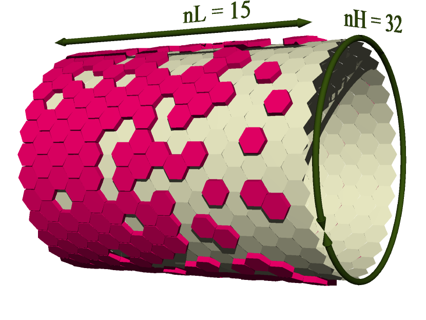
Figure 1: (Color online) 3D view of the first lattice geometry we used to test our results: a cylinder (lattice with periodic boundary conditions in one direction) connected to a full reservoir of cells (a source) on its left end and to an empty reservoir of cells (a sink) on its right end. Here, the system is made of $n_{L}+1=16$ rings of sites (including the two rings in the reservoirs), and each ring is made of $n_{H}=16$ sites. After some transient regime, a steady current of cells establishes along the cylinder. A typical configuration of the cells in the steady state for interaction parameter $p=0.8$ is shown.

In order to test the analytical results (13) and (14), we did some simulation of the cellular automaton in a simple geometry. More realistic simulations are the topic of the next Section. Since, as will be discussed later on, the equilibrium state of the cellular automaton is trivial (all configurations of the tumor cells are equally probable), we chose a setting where a nonequilibrium steady state of the tumor cells can exist: a cylinder made of $n_{L}+1$ rings of cells (its total length is $(n_{L}+1)a\sqrt{3}/2$) and base circumference $H=n_{H}a$ connected to a reservoir full of cells ($\rho=1$) at the left end and to an empty reservoir ($\rho=0$) at the right end, as shown in Fig. 1 ($n_{L}$ and $n_{H}$ are two integers). The first and the last ring of cells of the cylinder belong to the full and to the empty reservoirs respectively; hence the effective length over which diffusion takes place is $L:=n_{L}a\sqrt{3}/2$. We chose a cylinder rather than a simple rectangle in order to make the boundary effects in the direction perpendicular to the flow small, if not vanishing. We introduce two coordinates on the cylinder: $x$ is measured in the direction parallel to the axis and $y$ along the shortest circles. To simulate the reservoirs, on the boundaries of the system, cells behave under special evolution rules: each time one of the sites on the left border of the lattice is left by a cell, it becomes occupied again by a new cell with no delay, and each time a cell arrives on a site of the right border of the lattice, it is removed at once. In this geometry, if we let the system evolve starting from a random configuration, it relaxes to a steady state with a permanent current where gains and losses of cells from and to the two reservoirs compensate in average (but the instantaneous total number of cells still fluctuates as time advances). On an infinite lattice, the steady state might be reached only after an infinite duration. In practice, we simulate in parallel two families of independent systems, one where the site occupation probability is initially close to one and one where it is initially close to zero, and we stop our simulation when the values of the macroscopic observables (averaged over the systems of each family) are undistinguishable up to the error bars. The number of systems in each family is chosen so that the error bars are shorter than the precision that we request in advance.

In the steady state, the concentration profile can be computed in the macroscopic limit thanks to Fick’s law (17) or to the PDE (13). In the stationary regime (where no macroscopic quantity depends on time), any initial asymmetry has been “forgotten” by the system and $\rho(\vec{r})$ does not depend on $y$ because the system is translation-invariant in the $y$ direction. Furthermore, $\rho(\vec{r})$ is such that the current of cells is uniform: $\vec{\jmath}$, the density of cell current, is independent of $x$ and $y$. Then Fick’s law (17) reads

$$(2/\sqrt{3})D[\rho(x)]\,\partial_{x}\rho(x)=-j.$$ (19)

With the boundary conditions $\rho(0)=1$ and $\rho(L)=0$ and the expression for $D(\rho)$ above, we find in 2D

$$j=(1+p)/(6\sqrt{3}L)$$ (20)

and

$$x(\rho)=\{1+\rho[(2p-1)\rho(\rho-3)-3(1-p)]/(p+1)\}L.$$ (21)

Then one can get the curve for $\rho(x)$ by plotting the parametric curve $(x(\rho),\rho)$.

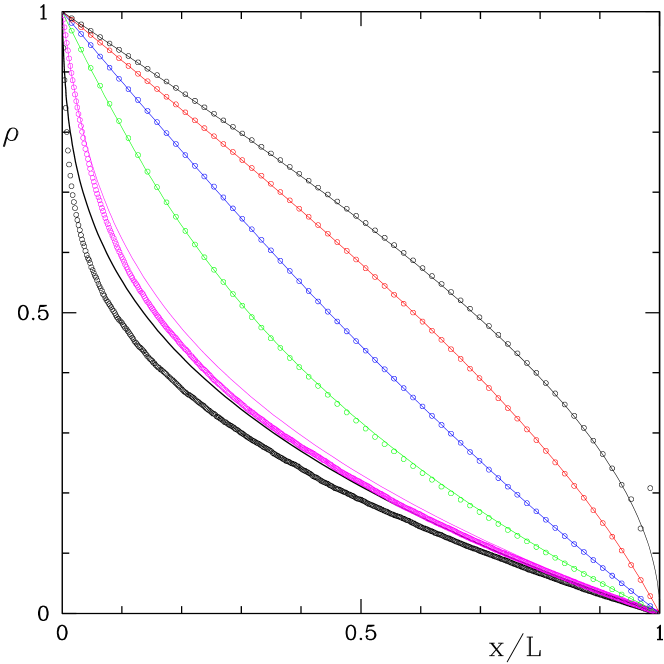
Figure 2: (Color online) Dependence on the interaction parameter $p$ of the stationary profiles $\rho(x/L)$ of the site occupation probability along the cylinder between the full reservoir (left, $x=0$, site occupation probability $\rho=1$) and the empty reservoir (right, $x=L$, $\rho=0$) — see Fig. (1). Since the cell concentration $c$ is proportional to the site occupation probability $\rho$, the profiles of $c$ would be the same. For each value of $p$, we plot the simulation results for the cellular automaton (circles) and our prediction from the analytic approximation Eq. (21) (solid lines). From bottom to top, $p=0.01$, 0.05, 0.2, 0.4, 0.7 and 1. The error bars are smaller than the circles’ size. The cylinder is made of $64\times 64$ sites except for $p=0.01$ and 0.05 where there are $512\times 512$ sites.

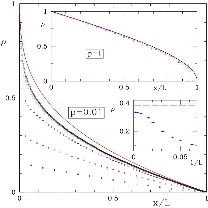
Figure 3: (Color online) Finite-size effects for the stationary profile of the cell concentration between the two reservoirs. Main curve: dots: profile $\rho(x/L)$ of the site occupation probability from simulation results for $p=0.01$ and system sizes $n_{L}=n_{H}-1=15$, 31, 63, 127, 255, and 511 (from bottom to top). It shows a strong finite-size dependence (for $p=0.05$, not shown, a weaker finite-size dependence is found). The solid line is the analytic approximation, clearly in disagreement with the simulation results. Bottom inset: for p=0.01, the extrapolation of the occupation probability $\rho$ at position $x=L/4$ to an infinite lattice shows that the discrepancy between the simulation data (dots) and the analytical approximation (dashed line) is not due to finite-size effects. Indeed, there is convergence toward a value of the site occupation probability that is clearly below the analytic approximation. Top inset: profile $\rho(x/L)$ for $p=1$, with numerical data for the sizes $n_{L}=15$, 31, and 63 only (dots) and analytic prediction (solid line). The finite-size effects are very weak and there is a good agreement between simulation data for large systems and the analytic prediction. This is true more generally for all values of $p$ away from 0 (say, larger than 0.1).

In Fig. 2, we plotted the stationary profile of the site occupation probability cell $\rho$ on the cylinder, between the two reservoirs, as obtained from simulations of the cellular automaton and from the macroscopic PDE. Notice the effect of nonlinear diffusion: for $p=1/2$ (not shown in Fig. 2), the profile is linear as predicted by the usual Fourier or Fick law, but, for other values of $p$, interactions between cells make it more complicated. For most values of $p$, there is an excellent agreement between the simulation results and the analytical approximation for all lattice sizes we tried (starting from $L=16$). However, we can distinguish two situations in which the microscopic and the macroscopic models disagree. The first one is related to a boundary effect: at the vicinity of the empty reservoir when $p=1$ (respectively at the vicinity of the full reservoir when $p=0$), a clear discrepancy of the average occupation probability $\rho$ of the last-but-one lattice site (respectively of the first few lattice sites) is seen between the cellular automaton results and the corresponding value from our analytic formula. The second situation is what happens when $p$ gets close to 0; see, e.g., $p=0.01$ and $0.05$ in Fig. 2. Here, the concentration profiles of the finite cellular automata show a strong finite-size dependence (main plot of Fig. 3, compared to the top inset of Fig. 3), and they seem to converge to some shape that is clearly different from the profile predicted from the PDE. To exclude the possibility that the simulation results agree with the analytic approximation at very large sizes, but not at the sizes we have simulated, we plot in the bottom inset of Fig. 3 an extrapolation to infinite systems: it shows that the discrepancy should persist even for huge systems. These phenomena are confirmed in Fig. 4, where the permanent current of cells across the cylinder is plotted as a function of $p$: one sees a good agreement for most values of $p$, with a slight deviation and practically no finite-size effects around $p=1$, and some more important deviation, together with strong finite-size effects, around $p=0$. This will be understood in the next subsection.

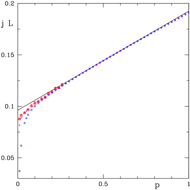
Figure 4: (Color online) Stationary current of cell density between the full and the empty reservoirs, across the cylinder (geometry defined in Fig. 1), as a function of the interaction parameter $p$. To be able to compare different system sizes (bottom to top : $nH-1=n_{L}=15$, 63 and 255), we actually plot the current density $j$ multiplied by the system length $L$ (dots). For $n_{L}=255$, only the points that differ significantly from the other sizes are represented. The error bars are smaller than the symbol’s sizes, except for $n_{L}=255$, where they are drawn. Solid line: analytic approximation, Eq. (20) times $L$. Like for the profile of the cell concentration, there is a large disagreement between the analytic approximation and the simulation results when $p$ is close to 0 and a small disagreement when $p$ is close to 1.

III.4 Discussion of our approximations: The occurrence of correlations

Our approximate computation of the hydrodynamic limit fails if the correlations between the occupation of neighboring sites are not negligible or if the continuous space limit has singularities (e.g., an infinite gradient) that cannot exist on the lattice.

III.4.1 Singularities in continuous space

Singularities are easy to predict and to address; they could happen for our model since the diffusion coefficient vanishes (for $p=1$ and $\rho=0$ on one hand and for $p=0$ and $\rho=1$ on the other). Indeed, Fick’s law reads

$$\vec{\jmath}(\vec{r},t)=-D[\rho(\vec{r},t)]\vec{\nabla}\rho(\vec{r},t),$$ (22)

and at a point where $D$ vanishes while $\vec{\jmath}$ is finite (which happens for $p=1$ or 0 between the two reservoirs of the previous subsection), the concentration gradient is infinite. To get the correct, physical behavior if necessary, it may suffice to reintroduce two or a few lattice sites around the point where the singularity appears and to solve separately the discrete equations (obtained after averaging but before the Taylor expansion) on these sites, and the PDE on the rest of the lattice.

In our case, this simple procedure does not enable one to quantitatively (or even qualitatively) understand the discrepancies between the automaton and the approximate results close to the reservoirs. This is because these discrepancies have to do with correlations.

III.4.2 Correlations

If $i$ and $j$ are two sites, let us consider the so-called connected correlation function  of $i$ and $j$,

$$\langle\rho_{i}(t)\rho_{j}(t)\rangle_{c} := \langle[\rho_{i}(t)-\langle\rho_{i}(t)\rangle][\rho_{j}(t)-\langle\rho_{j}(t)\rangle]\rangle$$ (23)

$$= \langle\rho_{i}(t)\rho_{j}(t)\rangle-\langle\rho_{i}(t)\rangle\langle\rho_{j}(t)\rangle.$$

This quantity is zero if the statistical distribution of the occupation numbers of the sites $i$ and $j$ is the same as if the sites $i$ and $j$ would be filled independently at random with given mean occupation probabilities. More precisely, in the case of a finite lattice of $N$ sites with a fixed total number of cells, this definition must be replaced with

$$\langle\rho_{i}(t)\rho_{j}(t)\rangle_{c}:=\langle[\rho_{i}(t)-\langle\rho_{i}(t)\rangle][\rho_{j}(t)-\langle N\rho_{j}(t)-1\rangle/(N-1)]\rangle$$ (24)

if one wants to detect correlations due to the interactions between cells that could be “hidden” behind the contribution $-\rho(1-\rho)/(N-1)$ due to the constraint that the total number of cells is fixed.

Our approximate computation of the hydrodynamic limit makes use of an assumption of statistical independence (“all connected correlations functions are zero”), and we found in our simulations that the correlations are indeed small (they vanish as $L\to+\infty$) in almost all cases.

A situation in which we can compute exactly the correlations is the equilibrium state of a translation invariant lattice. Since, in our stochastic automaton, any movement of a cell may be reversed and since, if the lattice is translation invariant, any transition from one configuration of the cells on the lattice to another has the same rate, $1/(6N)$, the detailed balance condition Ritort and Sollich (2003) is fulfilled, the equilibrium state exists, and the probability distribution of the configurations is uniform. Then the connected correlation functions (with the definition above, relevant to the case of conserved total cell number) between any two sites are zero. We simulated the cellular automaton in this situation and we checked that our numerical data are compatible with vanishing correlations (up to the error bars) for several values of $p$ and of the cell concentration; this is a check of correctness of the simulation program. In this case, our analytical approximation is exact, but the result is of course trivial ($\rho$ is uniform).

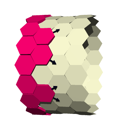
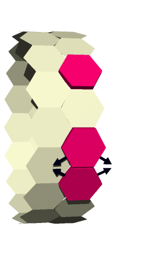
Figure 5: (Color online) Schematic explanation of the correlations that appear for $p$ close to 0 near the full reservoir (left) and for $p$ close to 1 near the empty reservoir (right). Left: when two cells sit next to one another close to the full reservoir and if $p$ is close to 0, they prevent one another from moving in one of the two directions that would be allowed if they were alone (black arrows represent permitted moves). Thus accompanied cells stay longer close to the reservoir than single ones, and positive correlations occur (see text). Right: when one cell sits close to the empty reservoir and if $p$ is close to 1, it cannot move unless it has a neighboring cell. Thus single cells stay longer close to the empty reservoir than accompanied ones, and negative correlations occur (see text).

Let us come back to the nonequilibrium steady state between the two reservoirs. In such a case, it is well known that correlations do exist, can be quantitatively important, and, above all, are generically long-range Spohn (1983); Garrido et al. (1990). For our automaton, we found numerically that, for $p$ close to 1 (0) there exists a significant negative (positive) correlation of the occupation probability of adjacent sites in the last (first) row of sites, parallel to the reservoir. This is why the macroscopic limit disagrees, in these situations, from the simulation. In other situations, they decrease at least as fast as $1/L$ as the system length $L$ goes to $+\infty$. Since studying these correlations in more detail would go beyond the scope of the present article, we limit ourselves here to explaining qualitatively what happens close to the boundaries. The correlation there can be interpreted using the microscopic rules (see Fig. 5). If $p=1$, when two cells are close to the empty, absorbing reservoir (Fig. 5 right), sooner or later one of the two cells will fall into the reservoir, leaving the other one alone. This other cell will not move until another cell comes on a neighboring site. Therefore, isolated cells stay longer close to the reservoir than accompanied cells, and there is more chance to find an empty site close to a cell than one would expect if cells were distributed at random, hence the negative correlations. Far away from the reservoir, the cell concentration is higher and there is always some cell to “unblock” an isolated cell, so the same phenomenon cannot be observed. Conversely, if $p=0$, when two cells are close to the full reservoir (Fig. 5, left), they are in some sense in each other’s way and they may progress away from the reservoir only in one of the two directions they could use if they were alone, the other direction being forbidden by the kinetic rule of the automaton since they would stay in contact with a cell they were already in contact with. If one could consider only these cells on the nearest line of sites from the reservoir and forget about the cells that lie on the next-to-nearest line of sites, one could conclude that accompanied cells stay longer close to the reservoir than single cells, that there is more chance to find another cell close to a cell than one would expect if cells were distributed at random, and that the correlation is positive. This is not so simple because the next-to-nearest line of sites has many cells that can compensate this effect, and we do observe that correlations extend over a few lines of sites away from the full reservoir, but the qualitative idea is correct. Far away from the full reservoir, the site occupation probability is not close to 1 and there is always some hole to “unblock” a cluster of cells, hence no such correlation is observed. We expect that taking into account these correlations into the analytic computation would improve the agremeent between simulations and analytic formulas.

Now let us come to the disagreement of the simulated and predicted concentrations of cells in the whole system when $p$ comes close to zero. Our interpretation is the following. We know from a preceding discussion that, at $p=0$, the cellular automaton is a cooperative KCM for which Fick’s law is obeyed only above some spatial scale that diverges with the cell concentration. Since, between the two reservoirs, all concentrations can be observed, Fick’s law might never hold even in arbitrarily large systems, but this is beyond the scope of the present paper. If $p$ is close to zero but strictly positive, we expect that the threshold spatial scale for effectively Brownian diffusion should be large (diverging with $p$) but finite at all values of the cell concentration. Therefore, and contrary to what happens for larger values of $p$ where the threshold scale must be comparable to the lattice spacing, there is a whole range of system sizes where the Brownian regime is not yet reached and the concentration profile depends strongly on the system size. Above this scale, diffusion sets in but, as a consequence of the cooperative nature of the kinetics, correlations always play a significant role and our evaluation of the diffusion constant, which neglects them, is irrelevant, hence the disagreement observed even at large system sizes between the predicted profile and the actual one.

IV Results for cells diffusing out of a spheroid

In this section, we come back to the radial geometry, where cells diffuse away from a center (cf. Sec. II B), in order to compare the results from the macroscopic model to experimental results. We use the expression of the diffusion coefficient obtained in Sec. III B 2, cf. Eq. (14), for a 2D system on a hexagonal lattice. We calculate numerically the solution of the nonlinear diffusion equation in a radial geometry by using a fully implicit method where the spatial derivatives in the diffusion equation are evaluated at time step $t+1$ (for the sake of stability) Press et al. (1992). The site occupation probability $\rho$ is constrained to be equal to $1$ in the center at all times.

A comparison between the density profiles from the automaton and from the numerical solution of the diffusion equation at the same time is presented in Fig. 6. As in the case of diffusion between a full and an empty reservoir, the agreement is very good except for $p=0.05$, close to the full reservoir, where the numerical solution does not agree with the density profile of the automaton as nicely as in the cases of larger $p$. This effect is due to correlations between close neighbors which are not negligible when $p$ is close to 0 (cf. Sec. III D 2). In general, the agreement between both profiles is nice. This is a supplementary check of our derivation of a nonlinear equation from the automaton.

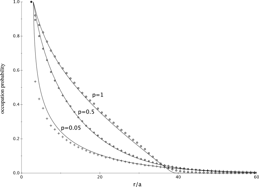
Figure 6: Density profiles from the automaton (dotted line) and from the numerical solution of the diffusion equation (full line) for $p=1$, $0.5$, and $0.05$. Error bars for the automaton density profile are smaller than the markers and thus are not represented.

This good agreement allows us to make a direct comparison between the numerical solution of the nonlinear diffusion equation and experimental cell densities. The experiments consisted in placing a spheroid of glioma cells (GL15) on a collagen substrate and following the evolution of the migration pattern during a few days. A detailed protocol has been described in  Aubert et al. (2006). Experiments have been performed by Christov at the Henri Mondor Hospital. Figure 7 is a photograph of an experimental spheroid, 36 h after cells started migrating. In order to compare the experimental density profiles at different times of evolution (cf. the full lines in Fig. 8) and the numerical solution of the diffusion equation, we rewrite Eq. (14) as

$$D(\rho)=D_{*}[2(1-p)+4(2p-1)\rho-2(2p-1)\rho^{2}],$$ (25)

where $D_{*}$ is the value of $D$ when $p=\frac{1}{2}$ (i.e., without interactions between cells). Note that $D_{*}=\frac{1}{8}$ when the time step of the numerical solution coincides with that of the automaton (cf. Sec. III B 2). For comparison with experimental data, the numerical time step is chosen equal to 1 h (and thus $D_{*}$ can be different from $\frac{1}{8}$). The spatial length step is set to $35.2~{}\mu$m as in the automaton, which corresponds to a characteristic size of cells. The diffusion equation was integrated for $p=0.95$. The choice $p=1$ induces sharp edges at low densities that do not correspond to our experimental profiles.

We find that, for the coefficient $D_{*}=1240\pm 100~{}{\mu\mathrm{m}}^{2}\,\mathrm{h}^{-1}$, numerical solutions at 12 and 36 h agree well with the experimental data at the same times, cf. Fig. 8. One can notice that this value falls within the range of values of the diffusion coefficient values obtained in vivo Swanson et al. (2008) (between 4 and $88~{}\mathrm{mm}^{2}/\mathrm{d}=450-10000~{}{\mu\mathrm{m}}^{2}\,\mathrm{h}^{-1}$), although this comparison must be taken with a grain of salt due to the different nature of the systems.

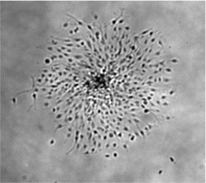
Figure 7: Experimental pattern of migration after 36 h. The real size of the image is $1.90\times 1.77$ mm.

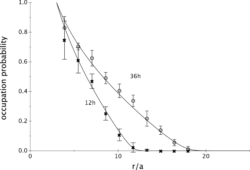
Figure 8: Comparison between the numerical solution of the nonlinear diffusion equation (full lines) and experimental data, at $t=12$ h (crosses) and $t=36$ h (circles). $D_{*}=1240\pm 100~{}{\mu\mathrm{m}}^{2}\,\mathrm{h}^{-1}$ with $a=35.2~{}\mu$m.

For this type of in vitro experiments, where cells are followed individually, the automaton remains the best way to model the system: time is counted as the number of cells that have left the spheroid, the lattice step corresponds to the mean size of a cell, and interaction between cells is represented by rules defined between neighboring cells. The only parameter to be fixed is $p$. On the contrary, for real tumors where the number of cells is of the order of $10^{7}$, the automaton becomes unmanageable, and in this case, the approach through a diffusion equation is more efficient.

V Conclusion and outlook

In this paper we set out to establish a link between a microscopic description of tumor cell migration with contact interactions (which we developed in Aubert et al. (2006)) and a macroscopic ones, based on diffusion-type equations used in most phenomenological models of tumor growth.

A microscopic description has obvious advantages. First, it allows a straightforward visualisation of the results: one “sees” the cells migrating. Moreover it can be directly compared to experiments and thus reveal special features of the migration like, for instance, cell attraction which we postulated in Aubert et al. (2006) in order to interpret the experimental cell distribution. It allows predictions for the trajectories of individual cells that can be observed in time-lapse microscopy experiments Druckenbrod and Epstein (2007); Young et al. (2004); Simpson et al. (2007). However the microscopic approach is not without its drawbacks. In all implementations we presented we have limited ourselves to a two-dimensional geometry. While a three-dimensional extension is, in principle, feasible it would lead to a substantial complication of the model. Moreover, even in a 2-D setting, it is not computationally feasible to accomodate the millions of cells present in a tumor. Our typical migration simulations involve at best a few thousand cells.

A macroscopic treatment on the other hand deals with mean quantities, like densities. Thus limitations such as the number of elementary entities (cells, in the present work) simply disappear. However the trace of microscopic interactions equally disappears unless it is explicitly coded into the macroscopic equations. This is a very delicate matter: the present work is dedicated to bridging just this gap between the microscopic and macroscopic approaches.

Our starting point was the microscopic description of cell migration which was validated through a direct comparison to experiment. Starting from a cellular automaton (with a given geometry and update rules) we have derived a nonlinear diffusion equation by taking the adequate continuous limits. Our main finding was that the interactions between cells modify the diffusion process inducing nonlinearities.

Such nonlinearities have been observed in models of ecosystems where individuals tend to migrate faster in overcrowded regions Okubo (1980); Murray (2002b). This mechanism (fleeing overcrowded regions) has also been the subject of speculation in the context of cell migration Witelski (1997), but, in our experimental situation, it is irrelevant: on one hand, cells in overcrowded regions cannot migrate fast, even if they want to, because they are fully packed (thus blocked); on the other hand it has been shown experimentally that the nonlinearity is due to attractive interactions between cells (when interactions are suppressed, the nonlinearity diminishes) Aubert et al. (2008).

While the present model is most interesting, it is fair to point out the precise assumptions that entered its derivation. We were based on a specific cellular automaton: many more do exist, the limit being only one’s imagination. Of course for the problem at hand it was essential to have a geometry allowing every site to possess a sufficiently large number of neighbours so as not to artificially hinder the cell motion. Moreover the update rules were chosen in fine through a comparison to experiment. But it would be interesting to see how robust the nonlinear diffusion coefficient is with respect to changes of the geometry: introducing a random deformation of the lattice or mimicking the migration of cancer cells on a susbtrate of astocytes in the spirit of Aubert et al. (2008). Moreover, if one forgets about the application to tumor cell migration, there may exist several interesting cases of cellular automaton geometry and kinetic rules leading to nonlinear diffusion equations worth studying, in addition to the kinetically constrained models we have seen and that have their own interest for the physics of glasses. We intend to come back to these questions in some future publications.

Finally, an incontrovertible generalization of the present work would be that of three-dimensional models. While the extension of microscopic models to three dimensions may be computationally overwhelming, the solution of three-dimensional diffusion equations, be they nonlinear, does not present particular difficulties. Thus once the automaton rules (mimicking the cell-cell interaction) have been used for the derivation of a diffusion equation like Eq. (13) with coefficient (15), we can proceed to the study of the macroscopic model, coupling diffusion to proliferation (plus, perhaps, other macroscopically described effects) for the modeling of real-life tumors (in particular, glioblastomas). This is a path we intend to explore in some future work.