Chaplygin ball over a fixed sphere: explicit integration

Abstract

We consider a nonholonomic system describing a rolling of a dynamically non-symmetric sphere over a fixed sphere without slipping. The system generalizes the classical nonholonomic Chaplygin sphere problem and it is shown to be integrable for one special ratio of radii of the spheres. After a time reparameterization the system becomes a Hamiltonian one and admits a separation of variables and reduction to Abel–Jacobi quadratures. The separating variables that we found appear to be a non-trivial generalization of ellipsoidal (spheroconic) coordinates on the Poisson sphere, which can be useful in other integrable problems.

Using the quadratures we also perform an explicit integration of the problem in theta-functions of the new time.

1 Introduction

One of the best known integrable systems of the classical nonholonomic mechanics is the Chaplygin problem on a non-homogeneous sphere rolling over a horizontal plane without slipping. In [8] S. A. Chaplygin obtained the equations of motion, proved their integrability and performed their reduction to quadratures by using spheroconical coordinates on the Poisson sphere as separating variables. He also actually solved the reconstruction problem by describing the motion of the sphere on the plane.

Various aspects of this celebrated system were studied in [4, 19, 8, 20], and its explicit integration in terms of theta-functions was presented in [17].

Several nontrivial integrable generalizations of this problem were indicated by V. Kozlov [21] (the motion of the sphere in a quadratic potential field), A. Markeev [23] (the sphere carries a rotator), in [25] (an extra nonholonomic constraint is added) and in [15] (the sphere touches an arbitrary number of symmetric spheres with fixed centers).

Next, amongst others, the papers [3, 4, 26] considered rolling of the Chaplygin (i.e., dynamically non-symmetric) sphere over a fixed sphere, so called sphere-sphere problem. They studied the equations of motion in the frame attached to the body. More generic (although more tedious) form of the equations also appeared in the works of Woronetz [27, 28], who, nevertheless, solved a series of interesting problems describing rolling of bodies of revolution or flat bodies over a sphere.

A rolling of a generic convex body over a sphere was also discussed in the recent survey [5].

In [3, 4, 26] it was observed that the equations of motion of the Chaplygin sphere-sphere problem admit an invariant measure, but, as numerical computations show, in the general case they are not integrable (there is no analog of the linear momentum integral). However, as was also found in [3], for one special ratio of radii of the two spheres an analog of such an integral does exist, and the system in integrable by the Jacobi last multiplier theorem.

Until recently, no one of the above generalizations was integrated in quadratures (except a case of particular initial conditions of the Kolzov generalization, considered in [14]).

In this connection it should be noted that a Lax pair with a spectral parameter for the Chaplygin sphere problem or for its generalizations is still unknown and, probably does not exists. Hence, one cannot use the powerful method of Baker–Akhieser functions to find theta-function solution of the problem.

Contents of the paper.

Our main purpose is to find appropriate separating variables, which allow to reduce the integrable case of the Chaplygin sphere-sphere problem to quadratures, as well as to give explicit theta-function solution.

It appears that, in contrast to the classical Chaplygin sphere problem, the usual spheroconical coordinates on the Poisson sphere do not provide separating variables and that such variables should be introduced in a more complicated way (see formulas (3.2)).

Using the quadratures, we also give a brief analysis of possible bifurcations and periodic solutions. These results are presented in Sections 3-4.

In Section 5 we briefly describe another type of periodic solutions.

Section 6 provides a derivation of explicit theta-function solutions of the problem in a self-contained form (Theorem 6.4).

Finally, in Appendix we show how the separating variables we used can be obtained in a systematic way, by reducing a restriction of our system to an integrable Hamiltonian system with 2 degrees of freedom and applying a classical result of Eisenhart on transformation of the Hamiltonian to a Stäckel form.

2 Equations of motion and first integrals

Consider rolling of the Chaplygin sphere inside/over a fixed sphere without slipping (Figure 1.)

Let $\boldsymbol{\omega}$, $m$, ${\bf I}={\rm diag}(I_{1},\,I_{2},\,I_{3})$, and $b$ denote respectively the angular velocity vector of the Chaplygin sphere, the mass of the sphere, its inertia tensor, and the radius.

By ${\boldsymbol{n}}$ we denote the unit normal vector to the fixed sphere $S^{2}$ at the contact point $P$. The angular momentum ${\boldsymbol{M}}$ of the moving sphere with respect to $P$ can be written as

$${\boldsymbol{M}}={\bf I}{\boldsymbol{\omega}}+d\,{\boldsymbol{n}}\times({\boldsymbol{n}}\times{\boldsymbol{\omega}}),\qquad d=mb^{2},$$ (2.1)

where $\times$ denots the vector product in ${\mathbb{R}}^{3}$.

The phase space of the dynamical system is the tangent bundle $T(SO(3)\times S^{2})$. By using the no slip nonholonomic constraint (which corresponds to zero velocity in the point of contact), one can obtain the reduced equations of motion in the frame attached to the sphere in the following closed form (see, e.g., [3]):

$$\dot{\boldsymbol{M}}={\boldsymbol{M}}\times\boldsymbol{\omega},\quad\dot{\boldsymbol{n}}=k\,{\boldsymbol{n}}\times\boldsymbol{\omega},\quad k=\frac{a}{a+b},$$ (2.2)

$a$ being the radius of the fixed sphere.

Note that the ratio $k$ can take any positive or negative value depending on the relative position of the rolling and fixed spheres, as illustrated in Fig. 1.

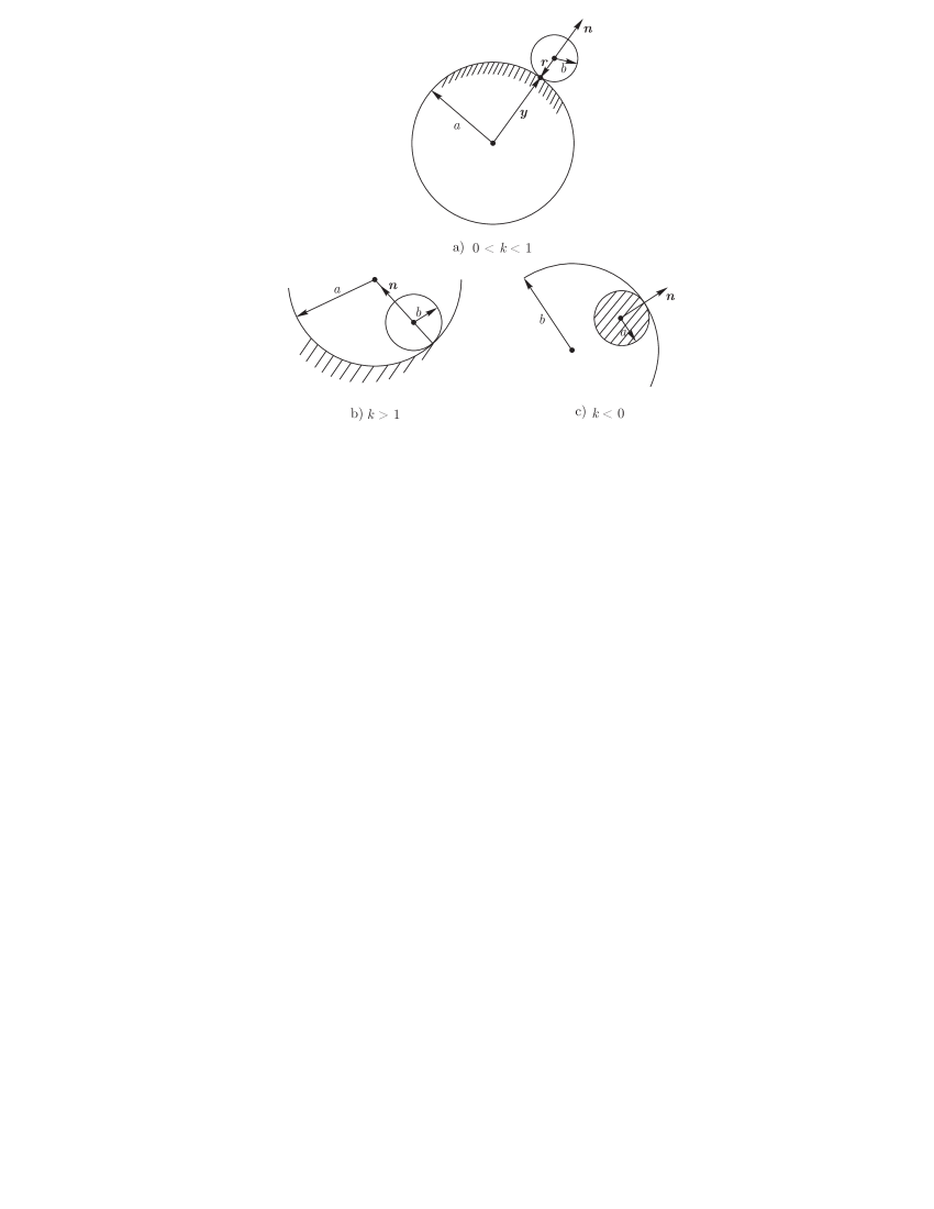
Figure 2.1: Rolling of the Chaplygin sphere inside/over the fixed sphere (dashed).

For arbitrary $k$ the equations (2.2) possess three independent integrals

$$F_{0}=\langle{\boldsymbol{n}},\,{\boldsymbol{n}}\rangle=1,\quad H=\langle{\boldsymbol{M}},\,{\boldsymbol{\omega}}\rangle,\quad F_{1}=\langle{\boldsymbol{M}},\,{\boldsymbol{M}}\rangle,$$ (2.3)

which, in view of (2.1), can be written as

$$F_{0} =\langle{\boldsymbol{n}},\,{\boldsymbol{n}}\rangle=1,\quad H=\langle\boldsymbol{\omega},{\bf J}\boldsymbol{\omega}\rangle-d^{2}\langle\boldsymbol{n},\boldsymbol{\omega}\rangle^{2},$$ (2.4)

$$F_{1} =\langle{\bf J}\boldsymbol{\omega},{\bf J}\boldsymbol{\omega}\rangle-2\langle{\bf J}\boldsymbol{\omega},\boldsymbol{n}\rangle\,\langle\boldsymbol{n},\boldsymbol{\omega}\rangle+d^{2}\langle\boldsymbol{n},\boldsymbol{\omega}\rangle^{2},$$

where ${\bf J}={\bf I}+d{\bf E}$, $\bf E$ being the identity matrix.

As shown in [26], the equations (2.2) expressed in terms of $omega,n$ also have the invariant measure $\rho\,d{\boldsymbol{\omega}}\,d{\boldsymbol{n}}$ with the density

$$\rho=\sqrt{\langle{\boldsymbol{n}},\,{\boldsymbol{n}}\rangle-d\langle{\boldsymbol{n}},\,{\bf J}^{-1}{\boldsymbol{n}}\rangle}.$$ (2.5)

Thus, according to the Jacobi theorem, for a complete integrability of this system one extra integral is needed.

The Chaplygin sphere on the plane.

Clearly, the case $k=1$ corresponds to $a\to\infty$, that is, the fixed sphere transforms to a horizontal plane with the unit normal vector $n$, and we arrive at the classical integrable Chaplygin problem, when the linear (in $M$) momentum integral is preserved:

$$\langle{\boldsymbol{M}},{\boldsymbol{n}}\rangle\equiv\langle{\bf I}{\boldsymbol{\omega}},{\boldsymbol{n}}\rangle.$$ (2.6)

Second integrable case.

According to [3], the system  (2.2) is also integrable in the case $k=-1$, which describes rolling of a non-homogeneous ball with a spherical cavity over a fixed sphere and the quotient of the radii of the spheres equals $\frac{b}{a}=\frac{1}{2}$ (see Fig. 1 c).

In this case, instead of (2.6), there is the following linear integral

$$F_{2}=\langle{\bf A}{\boldsymbol{M}},\,{\boldsymbol{n}}\rangle\,,$$ (2.7)

where

$${\bf A}={\rm diag}(J_{2}+J_{3}-J_{1},\,J_{3}+J_{1}-J_{2},\,J_{1}+J_{2}-J_{3})\,.$$

Note that, as was shown in [6], the modification of this system obtained by imposing the extra “no twist” constraint $\langle\boldsymbol{\omega},{\boldsymbol{n}}\rangle=0$ (sometimes called as the rubber Chaplygin ball) is also integrable for the ratio $k=-1$.

In the next sections we present explicit integration of this case under the condition $F_{2}=0$. Our procedure is similar to that of the problem of the Chaplygin sphere rolling on a horizontal plane in the case of zero value of the area integral (2.6), (see [8, 19, 7]), however, analytically, it is more complicated.

Integration of the system (2.2) with $k=-1$ in the general case $F_{2}\neq 0$ is still an open problem.

A remark on reduction to quadratures in the case $d=0$.

Note that in the limit case $d=0$ one has ${\boldsymbol{M}}={\bf I}\boldsymbol{\omega}$ and the equations (2.2) with $k=-1$ take the form

$${\bf I}\dot{\boldsymbol{\omega}}={\bf I}\boldsymbol{\omega}\times{\boldsymbol{\omega}},\quad\dot{\boldsymbol{n}}=-{\boldsymbol{n}}\times{\boldsymbol{\omega}}.$$

As was noticed in [3], by the substitution

$${\boldsymbol{\mathcal{M}}}={\bf AI}{\boldsymbol{\omega}},\quad{\boldsymbol{\gamma}}={\boldsymbol{n}}$$ (2.8)

and the sign change $t\to-t$, the latter system transforms to the Euler–Poisson equations for the classical Euler top,

$$\dot{\boldsymbol{\mathcal{M}}}={\boldsymbol{\mathcal{M}}}\times{\boldsymbol{\omega}},\quad\dot{\boldsymbol{\gamma}}={\boldsymbol{\gamma}}\times{\boldsymbol{\omega}},$$ (2.9)

$$\omega_{i}=a_{i}{\mathcal{M}}_{i},\quad a_{i}=\frac{1}{(J_{j}+J_{k}-J_{i})J_{i}},$$ (2.10)

which possesses first integrals

$$\langle{\boldsymbol{\mathcal{M}}},{\boldsymbol{\gamma}}\rangle=g,\quad\langle{\boldsymbol{\mathcal{M}}},{\boldsymbol{\mathcal{A}}}{\boldsymbol{\mathcal{M}}}\rangle=h,\quad\langle{\boldsymbol{\mathcal{M}}},{\boldsymbol{\mathcal{M}}}\rangle=f,$$

where ${\boldsymbol{\mathcal{A}}}=\rm{diag}(a_{1},a_{2},a_{3})$.

As was indicated in several publications (see, e.g., [16]), the Euler–Poisson equations (2.9) can be integrated by separation of variables. Namely, by an appropriate choice of the constant vector $\boldsymbol{\gamma}$ in space we can always set $g=0$. Then $\langle{\boldsymbol{\mathcal{A}}}\omega,{\boldsymbol{\gamma}}\rangle=0$, and the equations (2.9) reduce to a flow on the tangent bundle of the Poisson sphere $S^{2}=\{\langle{\boldsymbol{\gamma}},{\boldsymbol{\gamma}}\rangle=1\}$. In the spheroconical coordinates $\lambda_{1},\lambda_{2}$ on $S^{2}$ such that

$$\gamma_{i}^{2}=\frac{(a_{i}-\lambda_{1})(a_{i}-\lambda_{2})}{(a_{i}-a_{j})(a_{i}-a_{k})},\qquad i\neq j\neq k\neq i,$$ (2.11)

the flow is reduced to the quadratures

$$\begin{aligned} \frac{d\lambda_{1}}{\sqrt{R(\lambda_{1})}}+\frac{d\lambda_{2}}{\sqrt{R(\lambda_{2})}}&=0,\\ \frac{\lambda_{1}\,d\lambda_{1}}{\sqrt{R(\lambda_{1})}}+\frac{\lambda_{2}\,d\lambda_{2}}{\sqrt{R(\lambda_{2})}}&=C\,dt,\quad C=\mbox{const},\end{aligned}$$ (2.12)

$$R(\lambda)=-(\lambda-a_{1})(\lambda-a_{2})(\lambda-a_{3})(f\lambda-h).$$

The latter contain one holomorphic and one meromorphic differential on the elliptic curve ${\cal E}=\{\mu^{2}=R(\lambda)\}$. Thus the the quadratures give rise to a generalized Abel–Jacobi map and, following the methods developed in [10], they can be inverted to express the variables $\boldsymbol{\gamma},\boldsymbol{\omega}$ in terms of theta-functions of ${\cal E}$ and exponents (see, e.g., [18, 16] for the concrete expressions).

Apparently, in the general case $d\neq 0$ the substitution (2.8) is not useful to integrate the the equations (2.2) in the second integrable case $k=-1$. In particular, it does not transform these equations to the case of the classical Chaplygin sphere problem ($k=1$).

3 Reduction to quadratures in the case $F_{2}=0$

We now consider the case $d\neq 0$, but assume that the linear integral $F_{2}$ in (2.7) is zero, which imposes restrictions of the initial conditions. Then, from  (2.2) with $k=-1$ and $F_{2}=0$ we get

$$\dot{\boldsymbol{n}}=-{\boldsymbol{n}}\times\boldsymbol{\omega},\quad\langle\boldsymbol{\omega},{\bf B}\boldsymbol{n}\rangle=0,$$

where ${\bf B}=({\bf J}-d{\boldsymbol{n}}\otimes{\boldsymbol{n}}){\bf A}$. This allows to express the angular velocity in terms of $\dot{\boldsymbol{n}},{\boldsymbol{n}}$ in the following homogeneous form

$${\boldsymbol{\omega}}=\frac{{\bf B}{\boldsymbol{n}}\times\dot{\boldsymbol{n}}}{\langle{\boldsymbol{n}},\,{\bf B}{\boldsymbol{n}}\rangle}.$$ (3.1)

In view of the above remark on the reduction to quadratures in the case $d=0$, to perform separation of variables it seems natural to use the spheroconical coordinates $\lambda_{1},\,\lambda_{2}$ given by (2.11) (with $\gamma_{i}$ replaced by $n_{i}$) in the general case $d\neq 0$ too. However, this choice does not lead to success: after some calculations one can see that the first integrals $H,F_{1}$ have mixed terms in the derivatives $\dot{\lambda}_{1},\,\dot{\lambda}_{2}$.

It appears that a correct choice is given by the following quasi-spheroconical coordinates $z_{1},\,z_{2}$ on the Poisson sphere $\langle{\boldsymbol{n}},{\boldsymbol{n}}\rangle=1$:

$$n_{i}^{2}=\frac{1}{G(z_{1},z_{2})}\frac{\det{\bf I}}{(J_{i}-d)J_{j}J_{k}}\,\frac{(a_{i}-z_{1})(a_{i}-z_{2})}{(a_{i}-a_{j})(a_{i}-a_{k})}\,,\qquad(i,j,k)=(1,2,3),$$ (3.2)

where

$$G(z_{1},z_{2})=1-d({\rm Tr}{\bf J}-2d)(z_{1}+z_{2})+d(4\det{\bf J}-d\,{\rm Tr}({\bf JA}))z_{1}z_{2},$$ (3.3)

and, as in (2.10), $a_{i}=(A_{i}J_{i})^{-1}$. A systematic derivation of the substitution (3.2) is presented in Appendix.

Note that when $d=0$, the factor $G$ becomes 1 and the relation (3.2) takes the form of (2.11), that is, $z_{1},z_{2}$ do become the usual spheroconical coordinates on $S^{2}$.

We note that similar quasi-spheroconical coordinates were already used in [6, 5] to integrate the ”rubber” Chaplygin sphere-sphere problem.

In the above coordinates $z_{1},z_{2}$ one has

$$\rho^{2}=\langle({\bf I}\boldsymbol{n},{\bf J}^{-1}\boldsymbol{n}\rangle=\frac{\det{\bf I}}{\det{\bf J}}\frac{1}{G(z_{1},z_{2})},\quad\langle\boldsymbol{n},{\bf B}\boldsymbol{n}\rangle=\det{\bf I}\det{\bf A}\,\frac{z_{1}z_{2}}{G(z_{1},z_{2})}$$ (3.4)

and

$$\dot{n}_{i}=\frac{1}{2}\left(\frac{\dot{z}_{1}}{z_{1}-a_{i}}+\frac{\dot{z}_{2}}{z_{2}-a_{i}}-\frac{\dot{G}(z_{1},z_{2})}{G(z_{1},z_{2})}\right)n_{i}\,.$$ (3.5)

Then the expressions (3.1) yield

$$\omega_{i}=\frac{n_{j}n_{k}}{2}\frac{J_{j}-J_{k}}{J_{i}-d}\left[\frac{(1-dA_{i}z_{2})\dot{z}_{1}}{(1-a_{j}^{-1}z_{1})(1-a_{k}^{-1}z_{1})z_{2}}+\frac{(1-dA_{i}z_{1})\dot{z}_{2}}{(1-a_{j}^{-1}z_{2})(1-a_{k}^{-1}z_{2})z_{1}}\right]\,,$$ (3.6)

$$\langle\boldsymbol{\omega},\boldsymbol{n}\rangle=\frac{n_{1}n_{2}n_{3}\,(J_{1}-J_{2})(J_{2}-J_{3})(J_{3}-J_{1})\,G(z_{1},z_{2})}{2\det I}\left[\frac{\dot{z}_{1}}{\Phi(z_{1})z_{2}}+\frac{\dot{z}_{2}}{\Phi(z_{2})z_{1}}\right],$$ (3.7)

$$\Phi(z)=(a_{1}^{-1}z-1)(a_{2}^{-1}z-1)(a_{3}^{-1}z-1).$$

Substituting them, as well as (3.2), into the integrals $H,F_{1}$ in (2.4), after simplifications we get

$$H =(z_{1}-z_{2})\frac{\det{\bf I}}{4G^{2}(z_{1},z_{2})}\left[\frac{\Psi(z_{2})}{\Phi(z_{1})z_{2}^{2}}\dot{z}_{1}^{2}-\frac{\Psi(z_{1})}{\Phi(z_{2})z_{1}^{2}}\dot{z}_{2}^{2}\right]\,,$$ (3.8)

$$F_{1} =(z_{1}-z_{2})\frac{\det{\bf I}}{4G^{2}(z_{1},z_{2})}\left[\frac{\psi(z_{2})}{\Phi(z_{1})z_{2}^{2}}\dot{z}_{1}^{2}-\frac{\psi(z_{1})}{\Phi(z_{2})z_{1}^{2}}\dot{z}_{2}^{2}\right]\,$$

where

$$\Psi(z)=d\det{\bf A}z^{2}-{\rm Tr}({\bf AJ})z+2,\quad\psi(z)=(4\det{\bf J}-d\,{\rm Tr}({\bf AJ}))z-({\rm Tr}{\bf J}-2d).$$ (3.9)

Next, substituting (3.6), (3.7), and (3.2) into (2.1), we also obtain

$$M_{i}=\frac{n_{j}n_{k}}{2}(J_{k}-J_{j})\left[\frac{\dot{z}_{1}}{(1-a_{j}^{-1}z_{1})(1-a_{k}^{-1}z_{1})z_{2}}+\frac{\dot{z}_{2}}{(1-a_{j}^{-1}z_{2})(1-a_{k}^{-1}z_{2})z_{1}}\right].$$ (3.10)

Now, fixing the values of the integrals by setting $H=h,F_{1}=f$, then solving (3.8) with respect to $\dot{z}_{1}^{2},\dot{z}_{2}^{2}$ and using the relation

$$\Psi(z_{2})\psi(z_{1})-\Psi(z_{1})\psi(z_{2})=\det{\bf A}\,(z_{2}-z_{1})\,G(z_{1},z_{2}),$$ (3.11)

we get

$$\dot{z}_{\alpha}^{2} =-\frac{z_{\beta}^{2}\,G(z_{1},z_{2})}{(z_{1}-z_{2})^{2}}\frac{4\Phi(z_{\alpha})(f\Psi(z_{\alpha})+h\psi(z_{\alpha}))}{\det{\bf I}\det{\bf A}}$$

$$=-\frac{z_{\beta}^{2}\,G(z_{1},z_{2})}{(z_{1}-z_{2})^{2}}4(z_{\alpha}-a_{1})(z_{\alpha}-a_{2})(z_{\alpha}-a_{3})\,(f\Psi(z_{\alpha})+h\psi(z_{\alpha})),\quad(\alpha,\beta=(1,2).$$

After the time reparameterization

$$dt=\frac{1}{\sqrt{G(z_{1},z_{2})}}d\tau\equiv\sqrt{\frac{\det{\bf J}}{\det{\bf I}}\,\langle{\bf I}\boldsymbol{n},{\bf J}^{-1}\boldsymbol{n}\rangle}\,d\tau$$ (3.12)

the above relations give

$$\frac{dz_{1}}{d\tau}=\frac{z_{2}\sqrt{R(z_{1})}}{z_{1}-z_{2}},\quad\frac{dz_{2}}{d\tau}=\frac{z_{1}\sqrt{R(z_{2})}}{z_{2}-z_{1}},$$ (3.13)

$$R(z)=-(z-a_{1})(z-a_{2})(z-a_{3})\,(f\Psi(z)+h\psi(z)).$$

The latter are equivalent to the following Abel–Jacobi type quadratures

$$\frac{dz_{1}}{\sqrt{R(z_{1})}}+\frac{dz_{2}}{\sqrt{R(z_{2})}}=2d\tau,\quad\frac{z_{1}\,dz_{1}}{\sqrt{R(z_{1})}}+\frac{z_{2}\,dz_{2}}{\sqrt{R(z_{2})}}=0,$$ (3.14)

which contain 2 holomorphic differentials on the hyperelliptic genus 2 curve $\Gamma=\{w^{2}=R(z)\}$.

In view of (3.9), when $d\to 0$, the polynomial $R(z)$ becomes a degree 4 polynomial, and (3.14) reduce to the quadratures (2.12) for the Euler top problem, as expected.

It is interesting that, like in the integration of the original Chaplygin sphere problem presented in [8], the reparameterization factor in (3.12) coincides with the density (2.5) of the invariant measure. In the real motion this factor never vanishes, hence the reparameterization is non-singular.

Now substituting the above formulas for $\dot{z}_{1}^{2},\dot{z}_{2}^{2}$ into (3.10), (3.6) and simplifying, we express the angular momentum $M$ and the velocity $\omega$ in terms of $z_{1},z_{2}$ and the conjugated coordinates $w_{1},w_{2}$:

$$M_{i} =\frac{\sqrt{I_{j}I_{k}}\,I_{i}}{\sqrt{(J_{i}-J_{j})(J_{i}-J_{k})}}\,\frac{\sqrt{(a_{j}-z_{1})(a_{j}-z_{2})}\,\sqrt{(a_{k}-z_{1})(a_{k}-z_{2})}}{2\sqrt{G(z_{1},z_{2})}}$$

$$\qquad\times\frac{1}{z_{1}-z_{2}}\left[\frac{w_{1}}{(z_{1}-a_{j})(z_{1}-a_{k})}-\frac{w_{2}}{(z_{2}-a_{j})(z_{2}-a_{k})}\right].$$ (3.15)

$$\omega_{i} =\frac{\sqrt{I_{j}I_{k}}}{\sqrt{(J_{i}-J_{j})(J_{i}-J_{k})}}\,\frac{\sqrt{(a_{j}-z_{1})(a_{j}-z_{2})}\,\sqrt{(a_{k}-z_{1})(a_{k}-z_{2})}}{2\sqrt{G(z_{1},z_{2})}}$$

$$\qquad\times\frac{1}{z_{1}-z_{2}}\left[\frac{(z_{2}-1/(dA_{i})w_{1}}{(z_{1}-a_{j})(z_{1}-a_{k})}-\frac{(z_{1}-1/(dA_{i}))w_{2}}{(z_{2}-a_{j})(z_{2}-a_{k})}\right].$$ (3.16)

Next, the projection $\langle\boldsymbol{\omega},\boldsymbol{n}\rangle$ in (3.7) takes the form

$$\langle\boldsymbol{\omega},\boldsymbol{n}\rangle =J_{1}J_{2}J_{3}\sqrt{(z_{1}-a_{1})(z_{1}-a_{2})(z_{1}-a_{3})\,(z_{2}-a_{1})(z_{2}-a_{2})(z_{2}-a_{3})}$$

$$\qquad\times\frac{1}{z_{1}-z_{2}}\left[\frac{w_{1}}{(z_{1}-a_{1})(z_{1}-a_{2})(z_{1}-a_{3})}-\frac{w_{2}}{(z_{2}-a_{1})(z_{2}-a_{2})(z_{2}-a_{3})}\right].$$

Since

$$w_{\alpha} =\sqrt{-(z_{\alpha}-a_{1})(z_{\alpha}-a_{2})(z_{\alpha}-a_{3})\,(f\Psi(z_{\alpha})+h\psi(z_{\alpha}))}$$

$$=\sqrt{-(z_{\alpha}-a_{1})(z_{\alpha}-a_{2})(z_{\alpha}-a_{3})\,fd\det{\boldsymbol{A}}(z_{\alpha}-c_{1})(z_{\alpha}-c_{2})},$$

the latter relation also reads

$$\langle\boldsymbol{\omega},\boldsymbol{n}\rangle =J_{1}J_{2}J_{3}\sqrt{(c_{1}-z_{1})(c_{1}-z_{2})}\,\sqrt{(c_{2}-z_{1})(c_{2}-z_{2})}$$

$$\qquad\times\frac{-1}{z_{1}-z_{2}}\left[\frac{w_{1}}{(z_{1}-c_{1})(z_{1}-c_{2})}-\frac{w_{2}}{(z_{2}-c_{1})(z_{2}-c_{2})}\right].$$ (3.17)

In Section 6 we shall use the above expressions to obtain explicit theta-function solutions for the components of $n,\omega,M$ in terms of the new time $\tau$.

4 Qualitative study of the motion and bifurcations

For generic constants $h,f$ the polynomial $R(z)$ in (3.14) has simple roots $a_{i},c_{1},c_{2}$, and in the real motion the separating variables $z_{1},z_{2}$ evolve between them in such a way that $R(z_{1}),R(z_{2})$ remain non-negative. This corresponds to a quasiperiodic motion of the sphere.

In the sequel we assume that the moments of inertia $I_{1},I_{2},I_{3}$ corresponds to a physical rigid body, i.e., that the triangular inequalities $I_{i}+I_{j}>I_{k}$ are satisfies. For concreteness, assume also that $d<J_{1}<J_{2}<J_{3}$. This also implies $0<A_{3}<A_{2}<A_{1}$ and $0<a_{1}<a_{2}<a_{3}$.

As follows from the first expression in (3.4), in the real case the factor $G(z_{1},z_{2})$ is always positive. Hence, the right hand sides of (3.2) are positive and the coordinates $n_{i}$ are real and satisfy $\langle\boldsymbol{n},\boldsymbol{n}\rangle=1$ if and only if $z_{1}\in[a_{1},a_{2}]$ and $z_{2}\in[a_{2},a_{3}]$, like the usual spheroconical coordinates.

Next, we have

Proposition 4.1.

For the real motion, when the constants $h,f$ are positive, and for any $d,J_{i}$ satisfying the above inequalities, the roots $c_{1}\leq c_{2}$ never coincide and

$$c_{1}<a_{1}\quad\textup{and if $f/h=J_{i}$, then}\quad c_{1}=\frac{2d-A_{i}}{d\,A_{k}A_{j}}<a_{1},\quad c_{2}=a_{i}.$$

Proof. Set $f/h=\lambda\in{\mathbb{R}}$. The roots $c_{1},c_{2}$ coincide with those of $\Psi(z)\lambda+\psi(z)$ and have the form

$$c_{1,2}=\frac{{\rm Tr}({\bf AJ})(\lambda+d)\pm\sqrt{\mathcal{D}}}{d\det{\bf A}},$$ (4.1)

$${\mathcal{D}}=({\rm Tr}({\bf AJ}))^{2}(\lambda+d)^{2}-8d\det{\bf A}(\lambda+d)+4d\det{\bf A}{\rm Tr}{\bf J}.$$

The condition ${\cal D}=0$ gives a quadratic equation on $\lambda$, whose determinant equals $-d\det{\bf I}\det{\bf A}^{2}$, always a negative number. Hence ${\cal D}>0$ and $c_{1}<c_{2}$.

Next, in view of (4.1), the condition $c_{1}-a_{1}=0$ also leads to a quadratic equation for $\lambda$, again with always negative determinant. Then, evaluating $c_{1}-a_{1}$ for one value of $\lambda$, we find $c_{1}<a_{1}$ for any $\lambda\in{\mathbb{R}}$.

Finally, setting in (4.1) $\lambda=J_{i}$ and simplifying, we obtain the indicated above expressions for $c_{1},c_{2}$.

Combining the statement of Proposition 4.1 with the permitted positions of $z_{1},z_{2}$, we conclude that, depending on value of $c_{2}$,

$$z_{1}\in[a_{1},c_{2}],\;z_{2}\in[a_{2},a_{3}],\quad\mbox{or }\quad z_{1}\in[a_{1},a_{2}],\;z_{2}\in[c_{2},a_{3}].$$ (4.2)

Then, in view of (3.2), the vector $\boldsymbol{n}$ always fills a ring ${\mathcal{R}}$ on the unit sphere $S^{2}=\{\langle x,x\rangle=1\}$ between the lines of its intersection with the cone

$$\sum_{i=1}^{3}\frac{J_{i}-d}{J_{i}}\frac{x_{i}^{2}}{a_{i}-c_{2}}=0.$$

Periodic solutions with bifurcations.

As follows from Proposition 4.1, the only periodic solutions with bifurcations can occur when the root $c_{2}$ coincides with $a_{1},a_{2}$ or $a_{3}$. This happens under the initial conditions

$$\omega_{i}=\omega_{j}=0,\quad n_{k}=0,\qquad(i,j,k)=(1,2,3),$$

when the sphere performs a periodic circular motion with $n_{k}\equiv 0$ and one has $\langle\omega,n\rangle\equiv 0$, $H=J_{k}\omega_{k}$, $F_{1}=J_{k}^{2}\omega_{k}^{2}$, which yields $f/h=J_{k}$. Then, in view of the above proposition, $c_{2}=a_{k}$ and the polynomial $R(z)$ in (3.13) has the double root $a_{k}$, as expected.

When $\lambda=f/h$ leaves the interval $[J_{1},J_{3}]$, the root $c_{2}$ goes beyond of $[a_{1},a_{3}]$. Then for $R(z_{1}),R(z_{2})$ to be both positive, one of $z_{i}$ must violate the condition (4.2). This implies that in the real case the quotient $f/h$ belongs to $[J_{1},J_{3}]$, and the bifurcation diagram on the plane $(h,f)$ consists only of 3 rays $f/h=J_{1},J_{2},J_{3}$.

Note that, according to the results of [8], a similar situation takes place for the Chaplygin sphere on the horizontal plane.

The motion of the contact point on the fixed sphere.

As mentioned above, in the generic case with $F_{2}=0$ the contact point on the moving sphere given by the vector ${\boldsymbol{n}}$ belongs to the ring $\cal R$ on $S^{2}$.

Then the following natural question arises: does the contact point on the fixed sphere also belongs to a ring or it cover the whole sphere ? (Recall ([8]) that in the case of the Chaplygin sphere on a horizontal plane the contact point on the plane moves inside a strip, whose axis is orthogonal to the horizontal momentum vector.)

To study the above problem we assume, without loss of generality, that the radius $a$ of the fixed sphere is 1. Then the contact point on this sphere is given by the unit vector ${\boldsymbol{n}}$ as viewed in space.

To describe the spatial evolution of $\boldsymbol{n}$, introduce a fixed orthogonal frame $O\xi\eta\zeta$ with the center $O$ in the center of the fixed sphere and the “vertical” axis $O\zeta$ directed along the fixed momentum vector $\boldsymbol{M}$. Then, in view of (3.10), the projection of ${\boldsymbol{n}}$ on $O\zeta$ can be written in form

$$n_{\zeta} =\frac{1}{|\boldsymbol{M}|}\langle{\boldsymbol{n}},\boldsymbol{M}\rangle=\frac{1}{\sqrt{f}}a_{1}a_{2}a_{3}\,(J_{1}-J_{2})(J_{2}-J_{3})(J_{3}-J_{1})\,n_{1}n_{2}n_{3}$$

$$\quad\times\left[\frac{z_{1}\,\dot{z}_{1}}{(z_{1}-a_{1})(z_{1}-a_{2})(z_{1}-a_{3})z_{2}}+\frac{z_{2}\,\dot{z}_{2}}{(z_{2}-a_{1})(z_{1}-a_{2})(z_{1}-a_{3})z_{1}}\right],$$

which, following (3.2) and the expressions for ${\dot{z}}^{2}_{1},{\dot{z}}^{2}_{2}$, after a simplification, reads

$$n_{\zeta} =\frac{\sqrt{-1}}{\sqrt{f}}J_{1}J_{2}J_{3}\,\sqrt{(c_{1}-z_{1})(c_{1}-z_{2})}\,\sqrt{(c_{2}-z_{1})(c_{2}-z_{2})}$$

$$\quad\times\frac{1}{G(z_{1},z_{2})}\frac{-1}{z_{1}-z_{2}}\left[\frac{z_{2}w_{1}}{(z_{1}-c_{1})(z_{1}-c_{2})}-\frac{z_{1}w_{2}}{(z_{2}-c_{1})(z_{2}-c_{2})}\right].$$ (4.3)

It follows that the right hand side of (4.3) is a quasiperiodic function of time. One can show that under the conditions (4.2) and $c_{1}<a_{1}<a_{2}<a_{3}$, the function $n_{\zeta}(z_{1},w_{1},z_{2},w_{2})$ is real and, regardless to signs of the roots $w_{\alpha}=\sqrt{R(z_{\alpha})}$, the function $|n_{\zeta}|$ has the absolute maximum in one of the vertices of the quadrangle ${\cal Q}\subset(z_{1},z_{2})={\mathbb{R}}^{2}$ defined by (4.2). In two other vertices of ${\cal Q}$ this function is zero.

Calculating $|n_{\zeta}|$ in the vertices of ${\cal Q}$, we find that for $c_{2}\neq a_{i}$ its maximum is strictly less than 1. It follows that the trajectory $\boldsymbol{n}(t)$ on the fixed sphere lies between the “horizontal” planes $\zeta=\pm\nu$, $\nu<1$.

To describe the trajectory $\boldsymbol{n}(t)$ on the fixed sphere in the “longitudinal” direction, apart from the fixed momentum vector $\boldsymbol{M}$ it is good to know another fixed vector which can be expressed in terms of $\omega,\boldsymbol{n}$. However, it seems that such a vector does not exist, and for this reason we introduce the longitude angle $\psi$ between the axis $O\xi$ and the vertical plane spanned by $\boldsymbol{M}$ and $\boldsymbol{n}$. Introduce also the the longitudinal unit vector $\boldsymbol{u}=M\times\boldsymbol{n}/|\boldsymbol{M}\times\boldsymbol{n}|$. Then we find

$$\dot{\psi}=\frac{|\boldsymbol{M}|}{|\boldsymbol{M}\times\boldsymbol{n}|}\left\langle\boldsymbol{u},\frac{d}{dt}{\boldsymbol{n}}\right\rangle=|\boldsymbol{M}|\frac{\left\langle\boldsymbol{M}\times\boldsymbol{n},\frac{d}{dt}{\boldsymbol{n}}\right\rangle}{\langle\boldsymbol{M}\times\boldsymbol{n},\boldsymbol{M}\times\boldsymbol{n}\rangle},$$

where $\frac{d}{dt}{\boldsymbol{n}}$ is the absolute derivative of ${\boldsymbol{n}}$ expressed in the coordinates of the moving frame. In view of the second vector equation in (2.1) with $k=-1$,

$$\frac{d}{dt}{\boldsymbol{n}}=\dot{\boldsymbol{n}}+\omega\times{\boldsymbol{n}}=2\omega\times{\boldsymbol{n}}.$$

Hence, we get

$$\dot{\psi}=|\boldsymbol{M}|\frac{\left\langle\boldsymbol{M}\times\boldsymbol{n},2\omega\times{\boldsymbol{n}}\right\rangle}{\langle\boldsymbol{M}\times\boldsymbol{n},\boldsymbol{M}\times\boldsymbol{n}\rangle}.$$ (4.4)

Next, using the expressions (3.6), (3.10), we obtain

$$2(\omega\times\boldsymbol{n})_{i}=\frac{n_{i}(J_{i}-d)}{G}\left[\frac{dA_{j}A_{k}z_{2}+A_{i}-2d}{a_{i}^{-1}z_{1}-1}\dot{z}_{1}+\frac{dA_{j}A_{k}z_{1}+A_{i}-2d}{a_{i}^{-1}z_{2}-1}\dot{z}_{2}\right],$$

$$(\boldsymbol{M}\times\boldsymbol{n})_{i}=\frac{n_{i}(J_{i}-d)}{2G}\left[\frac{(2J_{j}J_{k}-dA_{i})z_{2}-1}{(a_{i}^{-1}z_{1}-1)z_{2}}\dot{z}_{1}+\frac{(2J_{j}J_{k}-dA_{i})z_{1}-1}{(a_{i}^{-1}z_{2}-1)z_{1}}\dot{z}_{2}\right],$$

$$(i,j,k)=(1,2,3).$$

Substituting these formulas into (4.4) and expressing the derivatives $\dot{z}_{\alpha}$ in terms of $z_{1},w_{1},z_{2},w_{2}$, one finds the derivative $\dot{\psi}$ as a symmetric function of $(z_{1},w_{1})$ and $(z_{2},w_{2})$, that is, as a quasiperiodic function of $t$. Its integration yields $\psi(t)$, which, together with (4.3), provides a complete description of the contact point on the fixed sphere.

5 A special case of periodic motion.

Apart from the particular case of the motion with $F_{2}=0$, there is another special case, when this integral takes the maximal value, that is, when ${\bf A}\boldsymbol{n}$ is parallel to the momentum vector $\boldsymbol{M}$. In this case $\boldsymbol{M}=h\,{\bf A}\boldsymbol{n}$, $h=$const. In view of (2.1), this implies

$${\bf J}\boldsymbol{\omega}-d\langle\boldsymbol{\omega},\boldsymbol{n}\rangle=h\,{\bf A}\boldsymbol{n}\quad\mbox{and}\quad\boldsymbol{\omega}=h{\bf J}^{-1}\left({\bf A}\boldsymbol{n}+\frac{d}{\rho^{2}}\langle{\bf A}\boldsymbol{n},{\bf J}^{-1}\boldsymbol{n}\rangle\right),$$ (5.1)

$\rho$ being the same as in (2.5).

Substituting the expression for $\omega$ into the second equation in (2.2) and simplifying, we get the following closed system for $n$:

$$\boldsymbol{n}=h\frac{J_{1}+J_{2}+J_{3}-2d}{F}\,(\boldsymbol{n}\times{\bf J}^{-1}\boldsymbol{n})\,.$$ (5.2)

It has two independent integrals $\langle\boldsymbol{n},\boldsymbol{n}\rangle$ and $\langle\boldsymbol{n},{\bf J}^{-1}\boldsymbol{n}\rangle$ or $\langle{\bf A}\boldsymbol{n},{\bf A}\boldsymbol{n}\rangle$, which implies that the factor $F$ is constant on the trajectories and that the system has the form of the Euler top equations. As a result, in the general case the components of $n$ and $\omega$ are expressed in terms of elliptic functions of the original time $t$ and their evolution is periodic.

This situation is similar to that of the special case of the motion of the Chaplygin sphere on a horizontal plane, when the momentum vector $\boldsymbol{M}$ is vertical, and when the solutions are elliptic in the original time.

6 Theta-function solutions in the case $F_{2}=0$.

In order to find explicit solutions for the components of $\omega,\boldsymbol{M},\boldsymbol{n}$, and other variables, we first remind some necessary basic facts on the Jacobi inversion problem and its solution.

Solving the Jacobi inversion problem by means of Wurzelfunktionen.

Consider an odd-order genus $g$ hyperelliptic Riemann surface $\Gamma$ obtained from the affine curve

$$\{\mu^{2}=R(\lambda)\},\qquad R(\lambda)=(\lambda-E_{1})\cdots(\lambda-E_{2g+1})\},$$

by adding one infinite point $\infty$. Let us choose a canonical basis of cycles ${\mathfrak{a}}_{1},\ldots,{\mathfrak{a}}_{g}$, ${\mathfrak{b}}_{1},\ldots,{\mathfrak{b}}_{g}$ on $\Gamma$ such that

$${\mathfrak{a}}_{i}\circ{\mathfrak{a}}_{j}={\mathfrak{b}}_{i}\circ{\mathfrak{b}}_{j}=0,\quad{\mathfrak{a}}_{i}\circ{\mathfrak{b}}_{j}=\delta_{ij},\qquad i,j=1,\ldots,g,$$

where $\gamma_{1}\circ\gamma_{2}$ denotes the intersection index of the cycles $\gamma_{1},\gamma_{2}$ (For real branch points see an example in Figure 6.1). Next, let $\bar{\omega}_{1},\dots,\bar{\omega}_{g}$ be the conjugated basis of normalized holomorphic differentials on $\Gamma$ such that

$$\oint_{{\mathfrak{a}}_{j}}{\bar{\omega}}_{i}=2\pi\jmath\,\delta_{ij},\qquad\jmath=\sqrt{-1}.$$

The $g\times g$ matrix of $b$-periods $B_{ij}=\oint_{{\mathfrak{b}}_{j}}\bar{\omega}_{i}$ is symmetric and has a negative definite real part. Consider the period lattice $\Lambda^{0}=\{2\pi\jmath{\mathbb{Z}}^{g}+B{\mathbb{Z}}^{g}\}$ of rank $2g$ in ${\mathbb{C}}^{g}=(Z_{1},\dots,Z_{g})$. The complex torus Jac$(\Gamma)={\mathbb{C}}^{g}/\Lambda^{0}$ is called the Jacobi variety (Jacobian) of the curve $\Gamma$. For a fixed point $P_{0}$ the Abel map

$${\cal A}:\Gamma\mapsto{\rm{Jac}}(\Gamma),\quad{\cal A}(P)=\int_{P_{0}}^{P}(\bar{\omega}_{1},\dots,\bar{\omega}_{g})^{T}$$

describes a natural embedding of the curve into its Jacobian.

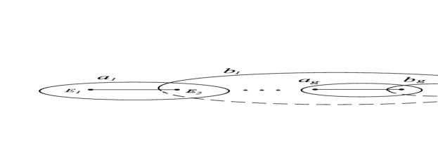
Figure 6.1: A canonical basis of cycles on the hyperelliptic curve represented as 2-fold covering of the complex plane $\lambda$. The parts on the cycles on the lower sheet are shown by dashed lines.

Now consider a generic divisor of points $P_{1}=(\lambda_{1},\mu_{1}),\ldots,P_{g}=(\lambda_{g},\mu_{g})$ on it, and the Abel–Jacobi mapping with a basepoint $P_{0}$

$$\int^{P_{1}}_{P_{0}}\bar{\omega}+\cdots+\int^{P_{g}}_{P_{0}}\bar{\omega}=Z,$$ (6.1)

$$\bar{\omega}=(\bar{\omega}_{1},\dots,\bar{\omega}_{g})^{T},\quad Z=(Z_{1},\ldots,Z_{g})^{T}\in{\mathbb{C}}^{g}.$$

Under the mapping, symmetric functions of the coordinates of the points $P_{1},\ldots,P_{g}$ are $2g$-fold periodic functions of the complex variables $Z_{1},\ldots,Z_{g}$ with the above period lattice $\Lambda^{0}$ (Abelian functions).

Explicit expressions of such functions can be obtained by means of theta-functions on the universal covering ${\mathbb{C}}^{g}=(Z_{1},\ldots,Z_{g})$ of the complex torus. Recall that customary Riemann’s theta-function $\theta(Z|B)$ associated with the Riemann matrix $B$ is defined by the series

$$\theta(Z|B)=\sum_{M\in{\mathbb{Z}}^{g}}\exp\langle\langle BM,M\rangle+\langle M,Z\rangle),$$ (6.2)

$$\langle M,Z\rangle=\sum^{g}_{i=1}M_{i}Z_{i},\quad\langle BM,M\rangle=\sum^{g}_{i,j=1}B_{ij}M_{i}M_{j}.$$

Equation $\theta(Z|B)=0$ defines a codimension one subvariety $\Theta\in\mbox{Jac}(\Gamma)$ (for $g>2$ with singularities) called theta-divisor.

We shall also use theta-functions with characteristics

$$\alpha=(\alpha_{1},\ldots,\alpha_{g}),\quad\beta=(\beta_{1},\ldots,\beta_{g}),\qquad\alpha_{j},\beta_{j}\in{\mathbb{R}},$$

which are obtained from $\theta(Z|B)$ by shifting the argument $Z$ and multiplying by an exponent:

$$\theta\!\left[{\alpha\atop\beta}\right]\!(Z)\equiv\theta\!\left[{\alpha_{1}\,\cdots\,\alpha_{g}\atop\beta_{1}\,\cdots\,\beta_{g}}\right]\!(Z)=\exp\{\langle B\alpha,\alpha\rangle/2+\langle Z+2\pi\jmath\beta,\alpha\rangle\}\,\theta(Z+2\pi\jmath\beta+B\alpha).$$

All these functions enjoy the quadiperiodic property

$$\theta\!\left[{\alpha\atop\beta}\right]\!(Z+2\pi\jmath K+BM)=\exp(2\pi\jmath\epsilon)\exp\{-\langle BM,M\rangle/2-\langle M,Z\rangle\}\theta\!\left[{\alpha\atop\beta}\right]\!(Z),$$ (6.3)

$$\epsilon=\langle\alpha,K\rangle-\langle\beta,M\rangle,$$

Now for a generic divisor $P_{1}=(\lambda_{1},\mu_{1}),\ldots,P_{g}=(\lambda_{g},\mu_{g})$ on $\Gamma$, introduce the polynomial $U(\lambda,s)=(s-\lambda_{1})\cdots(s-\lambda_{g})$, $\lambda\in{\mathbb{C}}$. It is known (see e.g., [1, 2]) that given a generic constant $C\neq E_{i}$, then under the Abel mapping (6.1) with $P_{0}=\infty$ the following relations hold

$$U(\lambda,C)\equiv(C-\lambda_{1})\cdots(C-\lambda_{g})=\varkappa\frac{\theta[\Delta](Z-q)\theta[\Delta](Z+q)}{\theta^{2}[\Delta](Z)},$$ (6.4)

$$q={\cal A}(C,\sqrt{R(C)})=\int_{\infty}^{(C,\sqrt{R(C)})}(\bar{\omega}_{1},\dots,\bar{\omega}_{g})^{T},$$

where $\varkappa$ is a constant depending on the periods of $\Gamma$ only.

These relation can be generalized in different ways as follows.

Theorem 6.1.

(see, e.g., [1, 2, 16]). Under the Abel mapping (6.1) with $P_{0}=\infty$ the following relations hold

$$\sqrt{U(\lambda,E_{i})}\equiv\sqrt{(E_{i}-\lambda_{1})\cdots(E_{i}-\lambda_{g})} =k_{i}\frac{\theta[\Delta+\eta_{i}](Z)}{\theta[\Delta](Z)},$$ (6.5)

$$\sum^{g}_{k=1}\frac{\mu_{k}}{\prod_{l\neq k}(\lambda_{k}-\lambda_{l})}\,\frac{\sqrt{U(\lambda,E_{i})}\,\sqrt{U(\lambda,E_{j})}}{(E_{i}-\lambda_{k})(E_{j}-\lambda_{k})} =k_{ij}\frac{\theta[\Delta+\eta_{ij}](Z)}{\theta[\Delta](Z)},$$ (6.6)

$$i,j=1,\dots,2g-1,\quad i \neq j,$$

where $k_{i},k_{ij}$ are certain constants depending on the periods of $\Gamma$ only, and

$$\Delta=\begin{pmatrix}\Delta^{\prime}\\ \Delta^{\prime\prime}\end{pmatrix},\quad\eta_{i}=\begin{pmatrix}\eta_{i}^{\prime}\\ \eta^{\prime\prime}_{i}\end{pmatrix},\qquad\Delta^{\prime},\Delta^{\prime\prime},\eta_{i}^{\prime},\eta^{\prime\prime}_{i}\in\frac{1}{2}{\mathbb{Z}}^{g}/{\mathbb{Z}}^{g}$$

are half-integer theta-characteristics such that

$$2\pi\jmath\,\eta_{i}^{\prime\prime}+B\eta_{i}^{\prime} =\int^{(E_{i},0)}_{\infty}\bar{\omega}\quad({\rm mod}\;\Lambda),$$ (6.7)

$$2\pi i\Delta^{\prime\prime}+B\Delta^{\prime} ={\cal K}\;({\rm mod}\;\Lambda),\quad\mbox{and}\quad\eta_{ij}=\eta_{i}+\eta_{j}\quad({\rm mod}\;{\mathbb{Z}}^{2g}),$$

${\cal K}\in{\mathbb{C}}^{g}$ being the vector of the Riemann constants.

Apparently, relations (6.6) were first obtained in the explicit form by Königsberger ([22]). Earlier, expressions (6.5) had been considered by K.Weierstrass as generalizations of the Jacobi elliptic functions ${\rm sn}(Z),{\rm cn}(Z)$, and dn$(Z)$. This set of remarkable relations between roots of certain functions on symmetric products of hyperelliptic curves and quotients of theta-functions with half-integer characteristics is historically referred to as Wurzelfunktionen (root functions).

One can show (see, e.g., [13, 1]) that for the chosen canonical basis of cycles ${\mathfrak{a}}_{1},\ldots,{\mathfrak{a}}_{g}$, ${\mathfrak{b}}_{1},\ldots,{\mathfrak{b}}_{g}$ on $\Gamma$,

$$\Delta^{\prime}=(1/2,\ldots,1/2)^{T},\quad\Delta^{\prime\prime}=(g/2,(g-1)/2,\ldots,1,1/2)^{T}\quad({\rm mod}\;1).$$ (6.8)

In the case $g=2$, all the functions in (6.5), (6.6) are single-valued on the 16-fold covering ${\mathbb{T}}^{2}\rightarrow$Jac$(\Gamma)$ with each of the four periods of $\Lambda_{0}$ doubled, so that ${\mathbb{T}}^{2}$ and Jac$(\Gamma)$ are transformed to each other by the change $Z\rightarrow 2Z.$ In view of (6.7), (6.8), one has

$$\Delta =\begin{pmatrix}1/2&1/2\cr 0&1/2\end{pmatrix},\quad\Delta+\eta_{1}=\begin{pmatrix}0&1/2\cr 0&1/2\end{pmatrix},\quad\Delta+\eta_{2}=\begin{pmatrix}0&1/2\cr 1/2&1/2\end{pmatrix},$$

$$\Delta+\eta_{3} =\begin{pmatrix}1/2&0\cr 1/2&1/2\end{pmatrix},\quad\Delta+\eta_{4}=\begin{pmatrix}1/2&0\cr 1/2&0\end{pmatrix},\quad\Delta+\eta_{5}=\begin{pmatrix}1/2&1/2\cr 1/2&0\end{pmatrix}.$$ (6.9)

We shall also need the following modification of the Königsberger formula (6.6), which, for our convenience, we adopt for the case $g=2$.

Theorem 6.2.

Let $C\in{\mathbb{C}}$ be a constant that does not coicide with $E_{i}$. Then under the Abel mapping (6.1) with $g=2$ and $P_{0}=\infty$:

$$\frac{1}{\lambda_{1}-\lambda_{2}}\left[\frac{\mu_{1}}{(E_{i}-\lambda_{1})(E_{j}-\lambda_{1})(C-\lambda_{1})}-\frac{\mu_{2}}{(E_{i}-\lambda_{2})(E_{j}-\lambda_{2})(C-\lambda_{2})}\right]$$

$$=\hat{k}_{ij}\frac{\theta^{2}[\Delta](Z)\;\theta[\Delta+\eta_{ij}](Z-q)\;\theta[\Delta+\eta_{ij}](Z+q)}{\theta[\Delta+\eta_{i}](Z)\;\theta[\Delta+\eta_{j}](Z)\;\theta[\Delta](Z-q)\,\theta[\Delta](Z+q)},$$ (6.10)

$$i,j=1,\dots,2g-1,\quad i\neq j,$$

where $\hat{k}_{ij}$ are constants depending on the periods of $\Gamma$ only and, as in (6.4), $q={\cal A}(C,\sqrt{R(C)})$.

Proof. Let us fix the point $P_{2}=(\lambda_{2},\mu_{2})$ in a generic position on the curve $\Gamma$ and consider the following meromorphic function on this curve

$$f(P)=\frac{\mu+\mu_{2}\frac{(\lambda-E_{i})(\lambda-E_{j})(\lambda-C))}{(\lambda_{2}-E_{i})(\lambda_{2}-E_{j})(\lambda_{2}-C)}}{(\lambda-\lambda_{2})(\lambda-E_{i})(\lambda-E_{j})(\lambda-C)}.$$

Due to the order of poles and zeros of $z,w$, and $\lambda-E_{i}$, $\lambda-C$ on $\Gamma$, for any generic $P_{2}$, the function $f(P)$ has simple poles at $P=P_{2},E_{i},E_{j},Q_{-},Q_{+}$ and does not have a pole neither at $\iota P_{2}=(\lambda_{2},-\mu_{2})$, nor at any other point on $\Gamma$. Next, $f(P)$ has a double zero at $\infty$. Then, using the description of zeros of $\theta(Z)$, $\theta[\Delta+\eta_{i}](Z),\theta[\Delta+\eta_{ij}](Z)$ one can show that up to a constant factor, $f(P)=\bar{f}(P)$ with

$$\bar{f}(P) =\frac{\theta^{2}[\Delta]({\cal A}(P)-{\cal A}(P_{2}))}{\theta[\Delta+\eta_{i}]({\cal A}(P)-{\cal A}(P_{2}))\,\theta[\Delta+\eta_{j}]({\cal A}(P)-{\cal A}(P_{2}))}$$

$$\quad\times\frac{\theta[\Delta+\eta_{ij}]({\cal A}(P)-q-{\cal A}(P_{2}))\,\theta[\Delta+\eta_{ij}]({\cal A}(P)+q-{\cal A}(P_{2}))}{\theta[\Delta]({\cal A}(P)-q-{\cal A}(P_{2}))\,\theta[\Delta]({\cal A}(P)+q-{\cal A}(P_{2}))}.$$

Note that due to the quasiperiodic property of the theta-functions with characteristics, $\bar{f}(P)$ is a meromorphic function on $G$.

Now setting $P=\iota P_{1}=(\lambda_{1},-\mu_{1})$, the function $-f(P)$ transforms to the left hand side of (6.10), and the argument ${\cal A}(P)-{\cal A}(P_{2})$ becomes $-Z$. Hence $\bar{f}(P)$ transforms to the right hand side of (6.10), which proves the theorem.

Combining Theorem 6.2 and formula (6.4), we obtain the following useful corollary.

Proposition 6.3.

Under the Abel mapping (6.1) with $g=2$ and $P_{0}=\infty$,

$$\frac{1}{\lambda_{1}-\lambda_{2}}\left[\frac{(C-\lambda_{2})\mu_{1}}{(E_{i}-\lambda_{1})(E_{j}-\lambda_{1})}-\frac{(C-\lambda_{1})\mu_{2}}{(E_{i}-\lambda_{2})(E_{j}-\lambda_{2})}\right]$$

$$={\rm const}_{ij}\frac{\theta[\Delta+\eta_{ij}](Z-q)\;\theta[\Delta+\eta_{ij}](Z+q)}{\theta[\Delta+\eta_{i}](Z)\,\theta[\Delta+\eta_{j}](Z)},$$ (6.11)

$$q={\cal A}(C,\sqrt{R(C)}),\qquad i,j=1,\dots,2g-1,\quad i\neq j,\quad C\neq E_{i}.$$

Proof. Indeed, the left hand side of (6.11) is obtained from that of (6.10) by multiplication by $(C-\lambda_{1})(C-\lambda_{2})$, whose theta-function expression is given by formula (6.4). Then the product of right hand sides of (6.10) and (6.4) gives (6.11).

Explicit theta-function solutions.

Now let $\Gamma$ be the genus 2 curve

$$\{w^{2}=R(z)\},\qquad R(z)=-(z-a_{1})(z-a_{2})(z-a_{3})\,(z-c_{1})(z-c_{2})\,,$$

$c_{1}<c_{2}$ being the roots of $f\Psi(z)+h\psi(z)$. Thus we identify (without order)

$$\{E_{1},\dots,E_{5}\}=\{a_{1},a_{2},a_{3},c_{1},c_{2}\},$$

and denote the corresponding half-integer characteristic $\eta_{i}$ by $\eta_{a_{i}}$ and $\eta_{c_{\alpha}}$.

Next, choose the canonical basis of cycles as depicted in Fig. 6.1 and calculate the $2\times 2$ period matrix

$$A_{ij}=\oint_{{\mathfrak{a}}_{j}}\varpi_{i},\qquad\varpi_{1}=\frac{dz}{\sqrt{R(z)}},\quad\varpi_{2}=\frac{z\,dz}{\sqrt{R(z)}}.$$

Then the normalized holomorphic differentials on $\Gamma$ are

$$\bar{\omega}_{k}=\sum_{j=1}^{2}C_{kj}\frac{z^{j-1}dz}{\sqrt{R(z)}},\qquad C=A^{-1},$$

and the quadratures (3.14) give

$$\int_{\infty}^{(z_{1},w_{1})}\bar{\omega}_{1}+\int_{\infty}^{(z_{2},w_{2})}\bar{\omega}_{1}=Z_{1},\quad\int_{\infty}^{(z_{1},w_{1})}\bar{\omega}_{2}+\int_{\infty}^{(z_{2},w_{2})}\bar{\omega}_{2}=Z_{2},$$ (6.12)

$$Z_{1}=2C_{11}\tau+Z_{10},\quad Z_{2}=2C_{21}\tau+Z_{20},$$ (6.13)

$Z_{10},Z_{20}$ being constant phases.

Now, comparing the last fraction in (3.2) with the expression (6.5) in Theorem 6.1, we find

$$S_{i}\equiv\frac{\sqrt{(a_{i}-z_{1})(a_{i}-z_{2})}}{\sqrt{(a_{i}-a_{j})(a_{i}-a_{k})}}=k_{i}\frac{\theta[\Delta+\eta_{a_{i}}](Z)}{\theta[\Delta](Z)},\qquad(i,j,k)=(1,2,3),$$ (6.14)

where $Z=(Z_{1},Z_{2})$ and the components of $Z$ depend on $\tau$ according to (6.13).

To calculate $k_{i}$, we set here $z_{1}=a_{j},z_{2}=a_{k}$. Then, in view of (6.12), the definition of $\theta$ with characteristics and the quasiperiodic property (6.3),

$$1=k_{i}\frac{\theta[\Delta+\eta_{a_{i}}]({\cal A}(a_{j})+{\cal A}(a_{k}))}{\theta[\Delta]({\cal A}(a_{j})+{\cal A}(a_{k}))}=k_{i}\frac{\theta[\Delta](0)}{\theta[\Delta+\eta_{a_{i}}](0)},\quad\mbox{that is,}\quad k_{i}=\frac{\theta[\Delta+\eta_{a_{i}}](0)}{\theta[\Delta](0)}.$$

In order to express in theta-functions the factor $G(z_{1},z_{2})$ given by (3.3), we fist note that it does not split into a product of linear functions in $z_{1}$ and $z_{2}$, hence one cannot use the formula (6.4).

On the other hand, from the condition $n_{1}^{2}+n_{2}^{2}+n_{3}^{2}\equiv 1$ we find that

$$G=\frac{\det{\bf I}}{\det{\bf J}}\left(\frac{J_{1}}{J_{1}-d}S_{1}^{2}+\frac{J_{2}}{J_{2}-d}S_{2}^{2}+\frac{J_{3}}{J_{3}-d}S_{1}^{2}\right),$$

which, in view of (6.14), gives

$$\sqrt{G(z_{1},z_{2})}=\sqrt{\frac{\det{\bf I}}{\det{\bf J}}}\,\frac{\sqrt{\Sigma(Z)}}{\theta[\Delta](Z)},$$ (6.15)

$$\Sigma(Z)=\frac{J_{1}}{I_{1}}\theta^{2}[\Delta+\eta_{a_{1}}](Z)+\frac{J_{2}}{I_{2}}\theta^{2}[\Delta+\eta_{a_{2}}](Z)+\frac{J_{3}}{I_{3}}\theta^{2}[\Delta+\eta_{a_{3}}](Z).$$

As a local singularity analysis shows, in general the function $\Sigma(Z)$ has zeros of first order, hence it cannot be a full square of another theta-function expression.

Now, using theta-function expressions (6.14), (6.15) in formulas (3.2), (3.15), (3.16) and applying also the Wurzelfunktionen (6.6), (6.11) with $C=1/(dA_{i})$, we arrive at the following theorem.

Theorem 6.4.

The generic theta-function solutions for the Chaplygin sphere-sphere problem in the case $F_{2}=0$ have the form

$$n_{i}(\tau) =\kappa_{i}\frac{\theta[\Delta+\eta_{a_{i}}](Z)}{\sqrt{\Sigma(Z)}},$$ (6.16)

$$M_{i}(\tau) =\nu_{i}\frac{\theta[\Delta+\eta_{a_{j}}+\eta_{a_{k}}](Z)}{\sqrt{\Sigma(Z)}},$$ (6.17)

$$\omega_{i}(\tau) =\varepsilon_{i}\frac{\theta[\Delta+\eta_{a_{j}}+\eta_{a_{k}}](Z-q_{i})\,\theta[\Delta+\eta_{a_{j}}+\eta_{a_{k}}](Z+q_{i})}{\theta[\Delta](Z)\cdot\sqrt{\Sigma(Z)}},$$ (6.18)

$$\qquad q_{i}={\cal A}(1/(dA_{i}),\sqrt{R(1/(dA_{i}))}),\quad\kappa_{i},\nu_{i},\varepsilon_{i}=\textup{const},\quad(i,j,k)=(1,2,3),$$

where the characteristics are given in (6.9) and $Z_{1},Z_{2}$ depend linearly on $\tau$ as described in (6.13).

We do not give explicit expressions for the constants $\kappa_{i},\nu_{i},\varepsilon_{i}$ here.

Note that due to presence of the square root, the variables $n_{i},M_{i},\omega_{i}$ are not meromorphic functions of $Z_{1},Z_{2}$ and therefore, of the new time $\tau$. This stays in contrast with the solutions of the classical Chaplygin sphere problem, which, after a similar time reparameterization, become meromorphic (see [11, 17]).

Next, comparing the expression (3.17) with the Wurzelfunktion (6.6) and (4.3) with (6.11), assuming $C=0$, we also find

$$\langle\boldsymbol{\omega},\boldsymbol{n}\rangle =\upsilon\frac{\theta[\Delta+\eta_{c_{1}}+\eta_{c_{2}}](Z)}{\theta[\Delta](Z)},$$ (6.19)

$$n_{\zeta} =\varrho\frac{\theta[\Delta+\eta_{c_{1}}+\eta_{c_{2}}](Z-\hat{q})\,\theta[\Delta+\eta_{c_{1}}+\eta_{c_{2}}](Z+\hat{q})}{\theta[\Delta](Z)\;\sqrt{\Sigma(Z)}},$$ (6.20)

$$\qquad\hat{q}={\cal A}(0,\sqrt{R(0)}),\qquad\upsilon,\varrho=\textup{const}.$$

The second formula, together with (6.13), describes the altitude of the contact point on the fixed sphere as a function of $\tau$.

Finally, given the expression (6.15) for the factor $G$, the original time $t$ can be found as a function of $\tau$ by integrating the quadrature (3.12).

Appendix. Separation of variables via reduction to a Hamiltonian system

As mentioned above, the substitution (3.2) is quite non-trivial and can hardly be guessed a priori. Below we describe how one can obtain it in a systematic way.

A1. Reduction to a Hamiltonian system on $S^{2}$

First introduce the spheroconical coordinates $u,\,v$ on the Poisson sphere $\langle{\boldsymbol{n}},{\boldsymbol{n}}\rangle=1$:

$$n_{i}^{2}=\frac{(J_{i}-u)(J_{i}-v)}{(J_{i}-J_{j})(J_{i}-J_{k})},\quad i\neq j\neq k\neq i,\quad J_{i}=I_{i}+d.$$ (6.21)

Then, under the substitution (3.1), the equations (2.2) with $k=-1$ give rise to the following Chaplygin-type system on $S^{2}$

$$\frac{d}{dt}\frac{\partial T}{\partial\dot{u}}-\frac{\partial T}{\partial u}=\dot{u}\Phi,\quad\frac{d}{dt}\frac{\partial T}{\partial\dot{v}}-\frac{\partial T}{\partial v}=-\dot{v}\Phi\,,$$ (6.22)

$$T=\frac{1}{2}(b_{uu}{\dot{u}}^{2}+b_{uv}{\dot{u}}{\dot{v}}+b_{vv}{\dot{v}}^{2}),\quad\Phi=(a_{u}{\dot{u}}+a_{v}{\dot{v}}),$$

where $T$ is the energy integral (2.3) expressed in the spheroconical coordinates under the condition $F_{2}=0$ and $\Phi$ is linear homogeneous in $\dot{u},\dot{v}$. Explicit expressions for the coefficients of $T,\,\Phi$ are quite tedious, so we do not give them here.

Introducing the momenta $P_{u}=\displaystyle\frac{\partial T}{\partial\dot{u}}$, $P_{v}=\displaystyle\frac{\partial T}{\partial\dot{v}}$, this system can be transformed to a Hamiltonian form with extra terms, which possesses invariant measure $N\,du\,dv\,dP_{u}\,dP_{v}$ with the density

$$N=\frac{2uv+(u+v)(2d+\alpha_{1})+\alpha_{2}-d\alpha_{1}}{\sqrt{\det({\bf J}-d{\boldsymbol{n}}\otimes{\boldsymbol{n}})}} (4\alpha_{3}+2\alpha_{1}\alpha_{2}-\alpha_{1}^{3}-d\alpha_{1}^{2}+$$

$$+ (\alpha_{1}^{2}-2\alpha_{2}+4d\alpha_{1})(u+v)-4d(u+v)^{2})^{-1},$$

where $\alpha_{1}=\sum J_{i},\,\alpha_{2}=\sum J_{i}^{2},\alpha_{3}=J_{1}J_{2}J_{3}$.

According to the Chaplygin theory of reducing multiplier ([8]), after the time reparameterization $N(u,\,v)\,dt=d\tau$ the system  (6.22) is transformed to the Lagrange form

$$\frac{d}{d\tau}\frac{\partial T}{\partial u^{\prime}}-\frac{\partial T}{\partial u}=0,\quad\frac{d}{d\tau}\frac{\partial T}{\partial v^{\prime}}-\frac{\partial T}{\partial v}=0,\qquad u^{\prime}=\frac{du}{d\tau},\quad v^{\prime}=\frac{dv}{d\tau}.$$ (6.23)

As a result, under the time reparameterization we obtain an integrable Hamiltonian system on the cotangent bundle $T^{*}S^{2}$ with local coordinates $u,v,p_{u}=\partial T/\partial u^{\prime},p_{v}=\partial T/\partial v^{\prime}$.

A2. Separation of variables

Equations (6.23) possess 2 homogeneous quadratic integrals, which come from $H,F_{1}$ (2.3) and which can be written in the form

$$H=T =\frac{1}{2}(g_{uu}(u^{\prime})^{2}+2g_{uv}u^{\prime}v^{\prime}+g_{vv}(v^{\prime})^{2}),$$

$$F_{1} =\frac{1}{2}(G_{uu}(u^{\prime})^{2}+2G_{uv}u^{\prime}v^{\prime}+G_{vv}(v^{\prime})^{2}).$$

Explicit expressions for the coefficients $g_{uu},\dots,G_{vv}$ as functions of $u,v$ are suppressed due to their complexity.

According to the result of Eisenhart [12] (see its modern accounting in [24]), separating variables $s_{1},s_{2}$ can be chosen as the roots of the equation

$$\det({\bf G}-s{\bf g})=0,$$ (6.24)

$${\bf G}=\begin{Vmatrix}G_{uu}&G_{uv}\\ G_{uv}&G_{vv}\\ \end{Vmatrix},{\bf g}=\begin{Vmatrix}g_{uu}&g_{uv}\\ g_{uv}&g_{vv}\\ \end{Vmatrix}.$$

Note that the roots depend only on the local coordinates $u,v$ on the configuration space $S^{2}$.

The spheroconical coordinates (6.21) depend explicitly on the roots $s_{1},s_{2}$ as follows

$$u=-\frac{1}{2}(y+\sqrt{y^{2}-4x}),\quad v=-\frac{1}{2}(y-\sqrt{y^{2}-4x}),$$

where

$$x=\frac{\pm s_{2}Q(s_{1})\pm s_{1}Q(s_{2})}{4d(s_{1}-s_{2})},\quad y=\frac{\pm Q(s_{1})\pm Q(s_{2})}{2d(s_{1}-s_{2})},$$

$$Q(s)=\sqrt{b_{1}s^{2}-b_{2}s+b_{3}^{2}},$$ (6.25)

$$b_{1}=\frac{1}{16}({\rm Tr}({\bf JA}))^{2}-\frac{1}{2}d\det{\bf A},\quad b_{3}=2\det{\bf J}-\frac{1}{2}d{\rm Tr}({\bf JA}),$$ (6.26)

$$b_{2}=\det{\bf J}{\rm Tr}({\bf JA})-\frac{1}{4}d({\rm Tr}({\bf JA}))^{2}-\frac{1}{2}d\det{\bf A}{\rm Tr}{\bf J}+d^{2}\det{\bf A}.$$ (6.27)

In the new variables $s_{1},s_{2}$ and the conjugated momenta $\displaystyle p_{1}=\frac{\partial T}{\partial s^{\prime}_{1}},p_{2}=\frac{\partial T}{\partial s^{\prime}_{2}}$ the integrals take the Liouville form

$$H=\frac{S_{1}(s_{1})}{s_{1}-s_{2}}p_{1}^{2}-\frac{S_{2}(s_{2})}{s_{1}-s_{2}}p_{2}^{2},\quad F_{1}=\frac{s_{2}S_{1}(s_{1})}{s_{1}-s_{2}}p_{1}^{2}-\frac{s_{1}S_{2}(s_{2})}{s_{1}-s_{2}}p_{2}^{2},$$ (6.28)

where

$$S(x) =\frac{2(8x^{3}+8(d-\epsilon)x^{2}+(2\epsilon^{2}\beta-4d\epsilon)x-4\gamma-d\beta+\sqrt{\Lambda(x)})}{\gamma(2x-\epsilon+2d)^{2}},$$ (6.29)

$$\Lambda =x^{2}(\beta^{2}+8\alpha d)+2x(4\beta\gamma+d\beta^{2}-2d\alpha\epsilon+4\alpha d^{2})+(4\gamma+d\beta)^{2},$$

and we used the notation

$$\alpha=(J_{2}+J_{1}-J_{3})(-J_{2}+J_{2}-J_{3})(-J_{2}+J_{2}+J_{3})=-A_{1}A_{2}A_{3},$$ (6.30)

$$\beta=J_{1}^{2}+J_{2}^{2}+J_{3}^{2}-2J_{1}J_{2}-2J_{2}J_{3}-2J_{3}J_{1}=-A_{1}A_{2}-A_{2}A_{3}-A_{3}A_{1},$$

$$\gamma=J_{1}J_{2}J_{3},\quad\epsilon=J_{1}+J_{2}+J_{3}.$$

Due to the Hamilton equations with the Hamiltonian $H$ in (6.28), the evolution of $s_{1},s_{2}$ is descibed as follows

$$s_{1}^{\prime}=\frac{\sqrt{2/\gamma}}{2s_{1}-e+2d}\frac{y_{1}}{s_{1}-s_{2}},\quad s_{2}^{\prime}=\frac{\sqrt{2/\gamma}}{2s_{2}-e+2d}\frac{y_{2}}{s_{2}-s_{1}},$$ (6.31)

$$y_{i}=\sqrt{Y(x_{i})},$$

$$Y(x)=\Lambda(x)\cdot(hx-f)\left[8x^{3}+8(d-e)x^{2}+(2e^{2}-\beta-4de)x-c+\sqrt{\Lambda(x)}\right],$$ (6.32)

where $h,f$ are the constants of the integrals $H,F_{1}$.

Hence, we performed a separation of variables, however the evolution equations (6.31) have a quite tedious form.

One can show that the equation $y^{2}=Y(x)$ defines an algebraic curve of genus 2 on the plane ${\mathbb{C}}^{2}=(x,y)$. According to the theory of algebraic curves, any curve of genus 2 is hyperelliptic and can be transformed to a canonical Weierstrass form by an appropriate birational transformation of the coordinates $x,y$.

One of such transformations is induced by the chain of substitutions $x\to\xi\to z$

$$x=\frac{4b_{3}\xi}{(\xi+b_{2})^{2}-4b_{1}b^{2}_{3}},\quad\xi=\frac{-(4\det{\bf J}-d{\rm Tr}(\bf{AJ}))\,z+{\rm Tr}\bf{J}-2d}{2\det{\bf A}\det{\bf I}},$$

$b_{1},b_{2},b_{3}$ being defined in (6.26), (6.27). It converts $\Lambda(x)$ in (6.32), as well as $Q(x)$ (6.25) into full squares.

After some tedious calculations, one finds that in the new variables $z_{1}=z(x_{1}),z_{2}=z(x_{2})$ the expressions (6.21) take the form (3.2), which ensures the reduction to hyperelliptic quadratures in the canonical form (3.14).

Acknowledgments

A.V.B. and I.S.M. research was partially supported by the Russian Foundation of Basic Research (projects Nos. 08-01-00651 and 07-01-92210). I.S.M. also acknowledges the support from the RF Presidential Program for Support of Young Scientists (MD-5239.2008.1). Yu.N.F. acknowledges the support of grant BFM 2003-09504-C02-02 of Spanish Ministry of Science and Technology.

References

- [1] Baker H.F. Abelian functions. Abel’s theorem and the allied theory of theta functions. Reprint of the 1897 original. Cambridge University Press, Cambridge, 1995
- [2] Buchstaber, V. M., Enol’skii, V.Z., and Leikin, D.V. Kleinian Functions, Hyperelliptic Jacobians and Applications, Amer. Math. Soc. Transl. Ser. 2, 179, Providence, USA, 1997.
- [3] Borisov, A.V. and Fedorov, Y.N. On Two Modified Integrable Problems of Dynamics, Vestnik Moskov. Univ. Ser. I Mat. Mekh., (1995), no. 6, 102–105 (in Russian).
- [4] Borisov, A.V. and Mamaev, I.S. The Rolling of Rigid Body on a Plane and Sphere. Hierarchy of Dynamics, Regul. Chaotic Dyn. 7, no. 1, (2002), 177–200.
- [5] Borisov, A.V. and Mamaev, I.S. Conservation Laws, Hierarchy of Dynamics and Explicit Integration of Nonholonomic Systems, Regul. Chaotic Dyn. 13, no. 5, (2008), 443–490.
- [6] Borisov, A.V. and Mamaev, I.S. Rolling of a Non-homogeneous Ball over a Sphere Without Slipping and Twisting. Regul. Chaotic Dyn. 12, no. 2, (2007), 153–159.
- [7] Borisov, A.V. and Mamaev, I.S. Isomorphism and Hamilton Representation of Some Nonholonomic Systems. Siberian Math. J. 48, no. 1, (2007), 26–36
- [8] Chaplygin, S.A. On a Ball’s Rolling on a Horizontal Plane, Matematicheskiĭ sbornik (Mathematical Collection) 24, (1903), [English translation: Regul. Chaotic Dyn. 7, no. 2, (2002), 131–148. http://ics.org.ru/eng?menu=mi_pubs&abstract=312.]
- [9] Chaplygin, S.A. On the Theory of Motion of Nonholonomic Systems. The Reducing-Multiplier Theorem, Matematicheskii sbornik (Mathematical Collection) 28, no. 1 (1911), [English transl.: Regul. Chaotic Dyn. 13, no. 4, (2008), 369–376; http://ics.org.ru/eng?menu=mi_pubs&abstract=1303].
- [10] Clebsch, A. and Gordan, P. Theorie der abelschen Funktionen, Leipzig: Teubner, 1866.
- [11] Duistermaat J.J. Chaplygin’s sphere. (2004) arXiv:math.DS/0409019
- [12] Eisenhart, L.P. Separable Systems of Stäckel. Annals of Mathematics 35, no. 2, (1934), 284–305.
- [13] Fay, J. Theta-Functions on Riemann Surfaces, Lecture Notes in Math., 352, New York: Springer-Verlag, 1973.
- [14] Fedorov, Yu. N, Integration of a Generalized Problem on the Rolling of a Chaplygin Ball, in Geometry, Differential Equations and Mechanics, Moskov. Gos. Univ., Mekh.-Mat. Fak., Moscow, 1985, 151–155.
- [15] Fedorov, Yu.N. Motion of a rigid body in a spherical suspension. Vestnik Moskov.Univ. Ser. I, Mat. Mekh. No. 5, (1988), 91–93. English transl.: Mosc. Univ. Mech. Bull. 43, No.5 (1988), 54–58
- [16] Fedorov, Yu. N. Classical integrable systems and billiards related to generalized Jacobians Acta Appl. Math. 55, no.3, (1999), 251–301
- [17] Fedorov, Yu. A Complete Complex Solution of the Nonholonomic Chaplygin Sphere Problem, Preprint, 2007.
- [18] Jacobi K.G. Sur la rotation d’un corps. In: Gesamelte Werke 2 (1884), 139–172
- [19] Kilin, A.A. The Dynamics of Chaplygin Ball: the Qualitative and Computer Analysis. Regul. Chaot. Dyn. 6 (3), (2001) 291–306
- [20] Kharlamov, A.P. Topologicheskii analiz integriruemykh zadach dinamiki tverdogo tela (Topological Analysis of Integrable Problems of Rigid Body Dynamics), Leningrad. Univ., 1988.
- [21] Kozlov, V.V. On the Integration Theory of Equations of Nonholonomic Mechanics, Adv. in Mech., 1985, 8, no. 3, pp. 85–107 (in Russian). English translation: Regul. Chaotic Dyn. 7, no. 2, (2002), 191–176.
- [22] Königsberger L. Zur Transformation der Abelschen Functionen erster Ordnung. J. Reine Agew. Math. 64 (1894), 3–42
- [23] Markeev A.P. Integrability of the problem of rolling of a ball with a non simply connected cavity filled by a fluid. Izv. Acad. Nauk SSSR Ser. Mekh. Tverd. Tela. 1 (1986), 64-65 (Russian)
- [24] Marikhin, V.G. and Sokolov, V.V. On the Reduction of the Pair of Hamiltonians Quadratic in Momenta to Canonic Form and Real Partial Separation of Variables for the Clebsch Top, Rus. J. Nonlin. Dyn. 4, no. 3 (2008), 313–322.
- [25] Veselov A.P., Veselova L.E. Integrable nonholonomic systems on Lie groups. (Russian) Mat. Zametki 44 (1988), no. 5, 604–619. English translation: Math. Notes 44 (1988), no. 5-6, 810–819 (1989)
- [26] Yaroshchuk, V.A. New Cases of the Existence of an Integral Invariant in a Problem on the Rolling of a Rigid Body, Without Slippage, on a Fixed Surface, Vestnik Moskov. Univ. Ser. I Mat. Mekh. no. 6, (1992), 26–30 (in Russian).
- [27] Woronetz, P. Über die rollende Bewegung einer Kreisscheibe auf einer beliebigen Fläche unter der Wirkung von gegebenen Kräften, Math. Annalen., 67, (1909), 268–280.
- [28] Woronetz, P. Über die Bewegung eines starren Körpers, der ohne Gleitung auf einer beliebigen Fläche rollt, Math. Annalen. 70, (1911), 410–453.