SUSY QCD impact on top-pair production associated with a $Z^{0}$-boson at a photon-photon collider

Abstract

The top-pair production in association with a $Z^{0}$-boson at a photon-photon collider is an important process in probing the coupling between top-quarks and vector boson and discovering the signature of possible new physics. We describe the impact of the complete supersymmetric QCD(SQCD) next-to-leading order(NLO) radiative corrections on this process at a polarized or unpolarized photon collider, and make a comparison between the effects of the SQCD and the standard model(SM) QCD. We investigate the dependence of the lowest-order(LO) and QCD NLO corrected cross sections in both the SM and minimal supersymmetric standard model(MSSM) on colliding energy $\sqrt{s}$ in different polarized photon collision modes. The LO, SM NLO and SQCD NLO corrected distributions of the invariant mass of $t\bar{t}$-pair and the transverse momenta of final $Z^{0}$-boson are presented. Our numerical results show that the pure SQCD effects in $\gamma\gamma\to t\bar{t}Z^{0}$ process can be more significant in the $+~{}+$ polarized photon collision mode than in other collision modes, and the relative SQCD radiative correction in unpolarized photon collision mode varies from $32.09\%$ to $-1.89\%$ when $\sqrt{s}$ goes up from $500~{}GeV$ to $1.5~{}TeV$.

PACS: 12.60.Jv, 14.70.Hp, 14.65.Ha, 12.38.Bx

I. Introduction

Although the standard model(SM)[1, 2] has achieved great success in describing all the available experiment data pertaining to the strong, weak and electromagnetic interaction phenomena, the elementary Higgs-boson, which is required strictly by the SM for spontaneous symmetry breaking, remains a mystery. Moreover, the SM suffers from some conceptional difficulties, such as the hierarchy problem, the necessity of fine tuning and the non-occurrence of gauge coupling unification at high energies. That has triggered an intense activity in developing extension models. The supersymmetric (SUSY) models can solve several conceptual problems of the SM by presenting an additional symmetry. For example, the quadratic divergences of the Higgs-boson mass can be cancelled by loop diagrams involving the SUSY partners of the SM particles exactly. Among all the SUSY extensions of the SM, the minimal supersymmetric standard model (MSSM)[3] is the most attractive one. Apart from the SUSY particle direct production, virtual effect of SUSY particle may also lead to observable deviations from the SM expectations. However, no direct experimental evidence of SUSY has been found yet.

The top-quark is the heaviest particle discovered up to now[4, 5], which was discovered by the CDF and D0 collaborations at Fermilab Tevatron ten years ago [6, 7]. It implies that the top-quark probably may play a special role in electroweak symmetry breaking (EWSB), and the observables involving top-quark may be closely connected with new physics. A possible signature for new physics can be demonstrated in the deviation of any of the couplings between the top-quarks and gauge bosons from the predictions of the SM. Until now there have been many works which devote to the effects of new physics on the observables related to the top-quark couplings in some extended models[8, 9, 10].

The International Linear Collider (ILC)[11] is an excellent tool to search for and investigate the extension models of the SM. The ILC is designed not only as an electron-positron collider, but also it provides another option as a photon-photon collider. The photon-photon collider is achieved by using Compton backscattered photons in the scattering of intense laser photons on the initial $e^{+}e^{-}$ beams. With the new possibility of $\gamma\gamma$ collisions at linear colliders, the anomalous coupling between top-quarks and $Z^{0}$-boson can also be probed by using $\gamma\gamma\to t\bar{t}Z^{0}$ process except via $e^{+}e^{-}\to t\bar{t}Z^{0}$ process[12, 13]. To detect a top-quark pair production associated with $Z^{0}$-boson at the ILC, the $\gamma\gamma\to t\bar{t}Z^{0}$ production channel has an outstanding advantage over $e^{+}e^{-}\to t\bar{t}Z^{0}$process due to its relative larger production rate. The reason is that the $e^{+}e^{-}\to t\bar{t}Z^{0}$process has a s-channel suppression from the virtual photon and $Z^{0}$ propagators at the tree-level, especially for the process with massive final particles [14, 15]. To the high energy $t\bar{t}Z^{0}$ production process, the SUSY radiative corrections, especially the SUSY QCD (SQCD) corrections, may be remarkable. We therefore study the full SQCD next-to-leading order (NLO) corrections to $t\bar{t}Z^{0}$ production in polarized and unpolarized $\gamma\gamma$ collisions in this paper.

In this work we calculate the NLO supersymmetric QCD corrections to the process $\gamma\gamma\to t\bar{t}Z^{0}$ in polarized and unpolarized photon-photon collision modes. We present also the calculation for the SM QCD NLO correction for comparison. The paper is arranged as follows: In section II we give the calculation description of the Born cross section. The calculations of full ${\cal O}(\alpha_{s})$ SQCD and SM QCD radiative corrections to the $\gamma\gamma\to t\bar{t}Z^{0}$ process are provided in section III. In section IV we present some numerical results and discussion, and finally a short summary is given.

II. LO calculation for $\gamma\gamma\to t\bar{t}Z^{0}$ process

The contributions to the cross section of process $\gamma\gamma\to t\bar{t}Z^{0}$ at the leading order(LO) in the MSSM model are of the order ${\cal O}(\alpha_{ew}^{3})$ with pure electroweak interactions. We generally make use of the ’t Hooft-Feynman gauge in the LO calculation, except in the calculation for the verification of the gauge invariance. There are totally six Feynman diagrams at the tree-level, which are generated by adopting FeynArts3.2 package[16] and shown in Fig.1. Each of these diagrams in Fig.1 includes a $Z^{0}$-boson bremsstrahlung originating from top-quark(or anti-top quark) line. The Feynman diagrams in Fig.1 can be topologically divided into t-channel(Fig.1(a,b,c)) and u-channel(Fig.1(d,e,f)) diagrams.

Figure 1: The lowest order diagrams for the $\gamma\gamma\to t\bar{t}Z^{0}$ process in both the SM and the MSSM model.

The notations for the process $\gamma\gamma\to t\bar{t}Z^{0}$ are defined as

$$\gamma(\lambda_{1},p_{1})+\gamma(\lambda_{2},p_{2})\to t(k_{1})+\bar{t}(k_{2})+Z^{0}(k_{3}).$$ (2.1)

All their momenta obey the on-shell equations $p_{1}^{2}=p_{2}^{2}=0$, $k_{1}^{2}=k_{2}^{2}=m_{t}^{2}$ and $k_{3}^{2}=m_{Z}^{2}$. The photon polarizations $\lambda_{1,2}$ can be $\pm 1$.

By applying FeynArts3.2 package, each Feynman diagram in Fig.1 is converted into corresponding amplitude as expressed below.

$${\cal M}_{0}^{(a)}(\lambda_{1},\lambda_{2}) = \frac{ie^{3}Q_{t}^{2}}{4s_{W}c_{W}}\times\frac{1}{\left(k_{1}-p_{1}\right)^{2}-m_{t}^{2}}\times\frac{1}{\left(p_{2}-k_{2}\right)^{2}-m_{t}^{2}}\bar{u}(k_{1})\hbox to0.0pt{/\hss}\epsilon\left(p_{1},\lambda_{1}\right)(\hbox to0.0pt{/\hss}k_{1}-\hbox to0.0pt{/\hss}p_{1}+m_{t})~{}~{}~{}~{}$$ (2.2)

$$\times \hbox to0.0pt{/\hss}\epsilon\left(k_{3}\right)\left(1-\gamma_{5}-\frac{8}{3}s_{W}^{2}\right)(\hbox to0.0pt{/\hss}p_{2}-\hbox to0.0pt{/\hss}k_{2}+m_{t})\hbox to0.0pt{/\hss}\epsilon\left(p_{2},\lambda_{2}\right)v(k_{2}),$$

$${\cal M}_{0}^{(b)}(\lambda_{1},\lambda_{2}) = \frac{ie^{3}Q_{t}^{2}}{4s_{W}c_{W}}\times\frac{1}{\left(k_{1}-p_{1}\right)^{2}-m_{t}^{2}}\times\frac{1}{\left(k_{2}+k_{3}\right)^{2}-m_{t}^{2}}\bar{u}(k_{1})\hbox to0.0pt{/\hss}\epsilon\left(p_{1},\lambda_{1}\right)(\hbox to0.0pt{/\hss}k_{1}-\hbox to0.0pt{/\hss}p_{1}+m_{t})~{}~{}~{}~{}$$ (2.3)

$$\times \hbox to0.0pt{/\hss}\epsilon\left(p_{2},\lambda_{2}\right)(-\hbox to0.0pt{/\hss}k_{2}-\hbox to0.0pt{/\hss}k_{3}+m_{t})\hbox to0.0pt{/\hss}\epsilon\left(k_{3}\right)\left(1-\gamma_{5}-\frac{8}{3}s_{W}^{2}\right)v(k_{2}),$$

$${\cal M}_{0}^{(c)}(\lambda_{1},\lambda_{2}) = \frac{ie^{3}Q_{t}^{2}}{4s_{W}c_{W}}\times\frac{1}{\left(k_{1}+k_{3}\right)^{2}-m_{t}^{2}}\times\frac{1}{\left(p_{2}-k_{2}\right)^{2}-m_{t}^{2}}\bar{u}(k_{1})\hbox to0.0pt{/\hss}\epsilon\left(k_{3}\right)\left(1-\gamma_{5}-\frac{8}{3}s_{W}^{2}\right)~{}~{}~{}~{}$$ (2.4)

$$\times (\hbox to0.0pt{/\hss}k_{1}+\hbox to0.0pt{/\hss}k_{3}+m_{t})\hbox to0.0pt{/\hss}\epsilon\left(p_{1},\lambda_{1}\right)(\hbox to0.0pt{/\hss}p_{2}-\hbox to0.0pt{/\hss}k_{2}+m_{t})\hbox to0.0pt{/\hss}\epsilon\left(p_{2},\lambda_{2}\right)v(k_{2}),$$

where $Q_{t}=2/3$ and the corresponding amplitudes of the u-channel Feynman diagrams(shown in Fig.1(d,e,f)) of the process $\gamma\gamma\to t\bar{t}Z^{0}$ can be obtained by making following interchanges.

$${\cal M}_{0}^{(d)}(\lambda_{1},\lambda_{2}) = {\cal M}_{0}^{(a)}(\lambda_{1},\lambda_{2})(p_{1}\leftrightarrow p_{2},\lambda_{1}\leftrightarrow\lambda_{2}),~{}~{}~{}~{}{\cal M}_{0}^{(e)}={\cal M}_{0}^{(b)}(\lambda_{1},\lambda_{2})(p_{1}\leftrightarrow p_{2},\lambda_{1}\leftrightarrow\lambda_{2}),~{}~{}~{}~{}$$ (2.5)

$${\cal M}_{0}^{(f)}(\lambda_{1},\lambda_{2})={\cal M}_{0}^{(c)}(\lambda_{1},\lambda_{2})(p_{1}\leftrightarrow p_{2},\lambda_{1}\leftrightarrow\lambda_{2}).$$

Finally, the total amplitude at the lowest order can be obtained by summing up all the above amplitudes.

$${\cal M}_{0}(\lambda_{1},\lambda_{2})=\sum_{i=a,b,c}^{d,e,f}{\cal M}_{0}^{(i)}(\lambda_{1},\lambda_{2}).$$ (2.6)

The $\gamma-\gamma$ collisions have five polarization modes: $+~{}+$, $+~{}-$, $-~{}+$, $-~{}-$ and unpolarized collision modes. The notation, for example, $+~{}-$ polarization represents the helicities of the two incoming photons being $\lambda_{1}=1$ and $\lambda_{2}=-1$, respectively. The cross sections of the $+~{}-$ and $-~{}+$ photon polarizations (i.e., J=2) are equal, and also the cross sections of the $+~{}+$ and $-~{}-$ photon polarizations (i.e., J=0) are the same. Therefore, in following calculation we concentrate ourselves only on the cross sections in $+~{}+$, $+~{}-$ and unpolarized photon-photon collision modes.

The differential cross sections for the process $\gamma\gamma\to t\bar{t}Z^{0}$ at the tree-level with polarized and unpolarized incoming photons are then obtained as

$$d\sigma_{0}(\lambda_{1},\lambda_{2}) = N_{c}\sum_{t\bar{t}Z}^{spins}|{\cal M}_{0}(\lambda_{1},\lambda_{2})|^{2}d\Phi_{3},$$ (2.7)

$$d\sigma_{0} = \frac{N_{c}}{4}\sum_{\lambda_{1},\lambda_{2}}\sum_{t\bar{t}Z}^{spins}|{\cal M}_{0}(\lambda_{1},\lambda_{2})|^{2}d\Phi_{3},$$ (2.8)

where $\sigma_{0}(\lambda_{1},\lambda_{2})$ is the tree-level cross section for polarized incoming photons with helicities of $\lambda_{1}$ and $\lambda_{2}$ respectively, $N_{c}=3$, and $\sigma_{0}$ is the Born cross section for unpolarized incoming photon beams. ${\cal M}_{0}(\lambda_{1},\lambda_{2})$ is the tree-level amplitude of all the diagrams shown in Fig.1 with $\lambda_{1}$ and $\lambda_{2}$ polarized photon beams. The first summation in Eq.(2.8) is taken over the polarization states of incoming photons, and the second summation over the spins of final particles $t\bar{t}Z^{0}$. The factor $\frac{1}{4}$ is due to taking average over the polarization states of the initial photons. $d\Phi_{3}$ is the three-particle phase space element defined as

$$d\Phi_{3}=\delta^{(4)}\left(p_{1}+p_{2}-\sum_{i=1}^{3}k_{i}\right)\prod_{j=1}^{3}\frac{d^{3}\textbf{{k}}_{j}}{(2\pi)^{3}2E_{j}}.$$ (2.9)

III. NLO SUSY QCD corrections to the $\gamma\gamma\to t\bar{t}Z^{0}$ process

The calculation of the one-loop diagrams is also performed in the conventional ’t Hooft–Feynman gauge. We use the dimensional regularization(DR) scheme to isolate the ultraviolet(UV) singularities. All the NLO SQCD corrections to the $\gamma\gamma\to t\bar{t}Z^{0}$ process in the MSSM come from the virtual correction and real gluon emission correction. And their Feynman diagrams can be divided into two parts: one is the SM-like part, another is the pure SQCD part. We take the definitions of one-loop integral functions as in Ref.[17], and adopt FeynArts3.2 package[16] to generate the SQCD one-loop Feynman diagrams and relevant counterterm diagrams of the process $\gamma\gamma\to t\bar{t}Z^{0}$ , and convert them to corresponding amplitudes. The FormCalc4.1 package[18] is applied to calculate the amplitudes of one-loop Feynman diagrams and get the numerical or analytical results. The relevant two-, three-, four- and five-point integrals are calculated by adopting our in-house programs developed from the FF package[19], these programs were verified in our previous works[13, 20, 21]. In these programs we used the analytical expressions for one-loop integrals presented in Refs.[22, 23, 24, 25]. At the SQCD NLO, there are 954 one-loop Feynman diagrams being taken into account in our calculation, and we depict all the pentagon diagrams in Fig.2. Figs.2(a-f) are the SM-like pentagon diagrams, and Figs.2(g-l) are the pure SQCD pentagon diagrams. The amplitude of the process $\gamma\gamma\to t\bar{t}Z^{0}$ including virtual SQCD corrections at ${\cal O}(\alpha_{s})$ order can be expressed as

$${\cal M}_{SQCD}={\cal M}_{0}+{\cal M}_{SQCD}^{vir}.$$ (3.1)

where ${\cal M}_{SQCD}^{vir}$ is the renormalized amplitude contributed by the full SQCD one-loop Feynman diagrams and their corresponding counterterms. The relevant renormalization constants for top field and mass are defined as

$$t_{0}^{L}=(1+\frac{1}{2}\delta Z_{t,{SQCD}}^{L})t^{L},~{}~{}t_{0}^{R}=(1+\frac{1}{2}\delta Z_{t,{SQCD}}^{R})t^{R},~{}~{}m_{t,0}=m_{t}+\delta m_{t}.$$ (3.2)

Taking the on-mass-shell renormalized condition we get the complete ${\cal O}(\alpha_{s})$ SQCD contributions of the renormalization constants as [27]

$$\delta Z_{t,{SQCD}}^{L} = \frac{\alpha_{s}C_{F}}{4\pi}\left[1-2B_{0}-2B_{1}+4m_{t}^{2}B_{0}^{{}^{\prime}}-4m_{t}^{2}B_{1}^{{}^{\prime}}\right](m_{t}^{2},0,m_{t}^{2})$$ (3.3)

$$+ \frac{\alpha_{s}C_{F}}{2\pi}\left\{\left[\cos^{2}\theta_{\tilde{t}}B_{1}+m_{t}m_{\tilde{g}}\sin(2\theta_{\tilde{t}})B_{0}^{{}^{\prime}}+m_{t}^{2}B_{1}^{{}^{\prime}}\right](m_{t}^{2},m_{\tilde{g}}^{2},m_{\tilde{t}_{1}}^{2})\right.$$

$$+ \left.\left[\sin^{2}\theta_{\tilde{t}}B_{1}-m_{t}m_{\tilde{g}}\sin(2\theta_{\tilde{t}})B_{0}^{{}^{\prime}}+m_{t}^{2}B_{1}^{{}^{\prime}}\right](m_{t}^{2},m_{\tilde{g}}^{2},m_{\tilde{t}_{2}}^{2})\right\},$$

$$\delta Z_{t,{SQCD}}^{R} = \frac{\alpha_{s}C_{F}}{4\pi}\left[1-2B_{0}-2B_{1}+4m_{t}^{2}B_{0}^{{}^{\prime}}-4m_{t}^{2}B_{1}^{{}^{\prime}}\right](m_{t}^{2},0,m_{t}^{2})$$ (3.4)

$$+ \frac{\alpha_{s}C_{F}}{2\pi}\left\{\left[\sin^{2}\theta_{\tilde{t}}B_{1}+m_{t}m_{\tilde{g}}\sin(2\theta_{\tilde{t}})B_{0}^{{}^{\prime}}+m_{t}^{2}B_{1}^{{}^{\prime}}\right](m_{t}^{2},m_{\tilde{g}}^{2},m_{\tilde{t}_{1}}^{2})\right.$$

$$+ \left.\left[\cos^{2}\theta_{\tilde{t}}B_{1}-m_{t}m_{\tilde{g}}\sin(2\theta_{\tilde{t}})B_{0}^{{}^{\prime}}+m_{t}^{2}B_{1}^{{}^{\prime}}\right](m_{t}^{2},m_{\tilde{g}}^{2},m_{\tilde{t}_{2}}^{2})\right\},$$

$$\frac{\delta m_{t}}{m_{t}} = -\frac{\alpha_{s}C_{F}}{4\pi}\left[(4B_{0}+2B_{1})(m_{t}^{2},m_{t}^{2},0)-1\right]$$ (3.5)

$$- \frac{\alpha_{s}C_{F}}{4\pi}\left\{\sum_{i=1}^{2}\left[B_{1}-(-1)^{i}\sin(2\theta_{\tilde{t}})\frac{m_{\tilde{g}}}{m_{t}}B_{0}\right](m_{t}^{2},m_{\tilde{g}}^{2},m_{\tilde{t}_{i}}^{2})\right\},$$

where $C_{F}=4/3$, $\theta_{\tilde{t}}$ is the scalar top mixing angle and $B_{0,1}^{{}^{\prime}}(p^{2},m_{1}^{2},m_{2}^{2})\equiv\frac{\partial B_{0,1}(p^{2},m_{1}^{2},m_{2}^{2})}{\partial p^{2}}$.

Figure 2: The NLO SQCD pentagon Feynman diagrams for the process $\gamma\gamma\to t\bar{t}Z^{0}$ in the MSSM model. The upper indexes in $\tilde{t}^{s,t}$ run from 1 to 2 respectively, which represent physical mass eigenstates $\tilde{t}_{1}$ and $\tilde{t}_{2}$. (a-f) are the SM-like pentagon diagrams, and (g-l) are the pure SQCD pentagon diagrams.

The total renormalized amplitude for all the one-loop Feynman diagrams is UV finite and without collinear IR singularity, but still contains soft IR singularity. If we regularize the soft IR divergence with a fictitious small gluon mass, then the virtual contribution of ${\cal O}(\alpha_{ew}^{3}\alpha_{s})$ order to the cross section of $\gamma\gamma\to t\bar{t}Z^{0}$ process with polarized and unpolarized incoming photons can be expressed as[4]

$$\Delta\sigma_{{\rm virtual}}(\lambda_{1},\lambda_{2}) = \sigma_{0}(\lambda_{1},\lambda_{2})\delta_{virtual}^{\lambda_{1},\lambda_{2}}$$ (3.6)

$$= \frac{(2\pi)^{4}N_{c}}{2|\vec{p}_{1}|\sqrt{s}}\int d\Phi_{3}\sum_{t\bar{t}Z}^{spins}{\rm Re}\left[{\cal M}_{0}^{{\dagger}}(\lambda_{1},\lambda_{2}){\cal M}_{SQCD}^{vir}(\lambda_{1},\lambda_{2})\right],$$

$$\Delta\sigma_{{\rm virtual}} = \sigma_{tree}\delta_{{\rm virtual}}$$ (3.7)

$$= \frac{(2\pi)^{4}N_{c}}{2|\vec{p}_{1}|\sqrt{s}}\int\frac{1}{4}d\Phi_{3}\sum_{\lambda_{1},\lambda_{2}}\sum_{t\bar{t}Z}^{spins}{\rm Re}\left[{\cal M}_{0}^{{\dagger}}(\lambda_{1},\lambda_{2}){\cal M}_{SQCD}^{vir}(\lambda_{1},\lambda_{2})\right],$$

where $N_{c}=3$ and $\vec{p}_{1}$ is spatial momentum in the center of mass system (c.m.s.) for one of the incoming photons. ${\cal M}_{SQCD}^{vir}(\lambda_{1},\lambda_{2})$ represents the renormalized amplitude of all the SQCD NLO Feynman diagrams with $\lambda_{1}$ and $\lambda_{2}$ polarized incoming photons. The phase space integration for $\gamma\gamma\to t\bar{t}Z^{0}$ process is implemented by using 2to3.F subroutine in FormCalc4.1 package. We checked the UV finiteness of the whole contributions from the virtual one-loop diagrams and counterterms both analytically and numerically by adopting non-zero small gluon mass. The soft IR divergence in the process $\gamma\gamma\to t\bar{t}Z^{0}$ is originated from virtual massless gluon corrections, which can be exactly cancelled by adding the real gluon bremsstrahlung corrections to this process in the soft gluon limit. The real gluon emission process is expressed as

$$\gamma(\lambda_{1},p_{1})+\gamma(\lambda_{2},p_{2})\to t(k_{1})+\bar{t}(k_{2})+Z^{0}(k_{3})+g(k_{4}).$$ (3.8)

We split the energy region of the real gluon radiated from the top or anti-top-quark into soft and hard regions, and apply the phase-space-slicing method [26] to isolate the soft gluon emission singularity for $\gamma\gamma\to t\bar{t}Z^{0}g$ process. That means the cross section for polarized photon beams can be decomposed into soft and hard terms

$$\Delta\sigma_{{real}}(\lambda_{1},\lambda_{2})=\Delta\sigma_{{soft}}(\lambda_{1},\lambda_{2})+\Delta\sigma_{{hard}}(\lambda_{1},\lambda_{2})=\sigma_{0}(\lambda_{1},\lambda_{2})(\delta_{{soft}}^{\lambda_{1},\lambda_{2}}+\delta_{{hard}}^{\lambda_{1},\lambda_{2}}).$$ (3.9)

Here we assume gluon being soft when $E_{g}\leq\Delta E_{g}$ and hard when $E_{g}>\Delta E_{g}$, where $\Delta E_{g}\equiv\delta_{s}E_{b}$, $E_{g}$ and $E_{b}=\sqrt{s}/2$ are the gluon energy and the photon beam energy respectively. The differential cross section of $\gamma\gamma\to t\bar{t}Z^{0}g$ in soft gluon energy range can be written as[27, 28]

$${\rm d}\Delta\sigma_{{\rm soft}}(\lambda_{1},\lambda_{2})=-{\rm d}\sigma_{0}(\lambda_{1},\lambda_{2})\frac{\alpha_{s}}{2\pi^{2}}\int_{|\vec{k}_{4}|\leq\Delta E_{g}}\frac{{\rm d}^{3}\vec{k}_{4}}{2k_{4}^{0}}\left[-\frac{k_{1}}{k_{1}\cdot k_{4}}+\frac{k_{2}}{k_{2}\cdot k_{4}}\right]^{2},$$ (3.10)

where the four-momentum of radiated gluon is denoted as $k_{4}=(E_{g},\vec{k}_{4})$. The soft contribution from Eq.(3.10) has an IR singularity at $m_{g}=0$, which can be cancelled with that from the virtual gluon corrections exactly. Therefore, the sum of the virtual and soft gluon emission corrections, is independent of the fictitious small gluon mass $m_{g}$. The hard gluon contribution is UV and IR finite, and can be computed directly by using the Monte Carlo method. We use our in-house $2\to 4$ phase space integration program to calculate the ${\cal O}(\alpha_{ew}^{3}\alpha_{s})$ order contribution to the cross section for hard gluon radiation process $\gamma\gamma\to t\bar{t}Z^{0}g$ . Finally, the corrected total cross section for the $\gamma\gamma\to t\bar{t}Z^{0}$ in $\lambda_{1}$, $\lambda_{2}$ polarized photon collisions($\sigma_{tot}^{\lambda_{1},\lambda_{2}}$) up to the order of ${\cal O}(\alpha^{3}_{ew}\alpha_{s})$, is obtained by summing up the ${\cal O}(\alpha^{3}_{ew})$ Born cross section($\sigma_{0}(\lambda_{1},\lambda_{2})$), the NLO SQCD virtual correction part($\Delta\sigma_{virtual}(\lambda_{1},\lambda_{2})$), and the ${\cal O}(\alpha^{3}_{ew}\alpha_{s})$ contribution from real gluon emission process $\gamma\gamma\to t\bar{t}Z^{0}g$ ($\Delta\sigma_{real}(\lambda_{1},\lambda_{2})$).

$$\sigma_{tot}^{\lambda_{1},\lambda_{2}} = \sigma_{0}(\lambda_{1},\lambda_{2})+\Delta\sigma_{{\rm tot}}(\lambda_{1},\lambda_{2})=\sigma_{0}(\lambda_{1},\lambda_{2})+\Delta\sigma_{{\rm virtual}}(\lambda_{1},\lambda_{2})+\Delta\sigma_{{\rm real}}(\lambda_{1},\lambda_{2})$$ (3.11)

$$= \sigma_{0}(\lambda_{1},\lambda_{2})\left(1+\delta_{SQCD}^{\lambda_{1},\lambda_{2}}\right),$$

where $\delta_{SQCD}^{\lambda_{1},\lambda_{2}}$ is the full ${\cal O}(\alpha_{s})$ SQCD relative correction to the $\gamma\gamma\to t\bar{t}Z^{0}$ process with $\lambda_{1}$, $\lambda_{2}$ polarized photon beams.

IV. Numerical Results and Discussion

In our numerical calculation, we take the relevant parameters as[29]: $\alpha_{{\rm ew}}(m_{Z}^{2})^{-1}=127.918$, $m_{W}=80.403~{}GeV$, $m_{Z}=91.1876~{}GeV$, $m_{t}=174.2~{}GeV$, $m_{u}=m_{d}=66~{}MeV$, $\sin^{2}\theta_{W}=1-m_{W}^{2}/m_{Z}^{2}=0.222549$, and the energy scale $\mu=m_{t}+\frac{1}{2}m_{Z}$. There we use the effective values of the light quark masses ($m_{u}$ and $m_{d}$) which can reproduce the hadron contribution to the shift in the fine structure constant $\alpha_{\rm ew}(m_{Z}^{2})$[30]. The 3-loop evolution of strong coupling constant $\alpha_{s}(\mu^{2})$ in the $\overline{MS}$ scheme with parameters $\Lambda_{QCD}^{n_{f}=5}=203.73~{}MeV$, yielding $\alpha_{s}^{\overline{MS}}(m_{Z}^{2})=0.1176$.

In the MSSM, the mass term of the scalar top quarks can be written as

$$-{\cal L}_{\tilde{t}}^{mass} = \left(\begin{array}[]{cc}\tilde{t}^{\ast}_{L}&\tilde{t}^{\ast}_{R}\end{array}\right){\cal M}^{2}_{\tilde{t}}\left(\begin{array}[]{c}\tilde{t}_{L}\\ \tilde{t}_{R}\end{array}\right),$$ (4.4)

where ${\cal M}^{2}_{\tilde{t}}$ is the mass matrix of $\tilde{t}$ squared, expressed as

$${\cal M}^{2}_{\tilde{t}} = \left(\begin{array}[]{cc}m^{2}_{\tilde{t}_{L}}&m_{t}a_{t}\\ a^{{\dagger}}_{t}m_{t}&m^{2}_{{\tilde{t}}_{R}}\end{array}\right),$$ (4.7)

and

$$m_{\tilde{t}_{L}}^{2} = M_{\tilde{Q}}^{2}+(I^{3L}_{t}-Q_{t}\sin^{2}\theta_{W})\cos 2\beta m_{Z}^{2}+m_{t}^{2},$$

$$m_{\tilde{t}_{R}}^{2} = M_{\tilde{U}}^{2}+Q_{t}\sin^{2}\theta_{W}\cos 2\beta m_{Z}^{2}+m_{t}^{2},$$

$$a_{t} = A_{t}-\mu(\tan\beta)^{-2I^{3L}_{t}},$$ (4.9)

where $M_{\tilde{Q}}$ and $M_{\tilde{U}}$ are the soft SUSY breaking masses, $I_{t}^{3L}$ is the third component of the weak isospin of the top quark, and $A_{t}$ is the trilinear scalar coupling parameter of Higgs-boson and scalar top-quarks, $\mu$ the higgsino mass parameter.

The mass matrix ${\cal M}_{\tilde{t}}$ can be diagonalized by introducing an unitary matrix ${\cal R}^{\tilde{t}}$. The mass eigenstates $\tilde{t}_{1}$, $\tilde{t}_{2}$ are defined as

$$\left(\begin{array}[]{c}\tilde{t}_{1}\\ \tilde{t}_{2}\end{array}\right)={\cal R}^{\tilde{t}}\left(\begin{array}[]{c}\tilde{t}_{L}\\ \tilde{t}_{R}\end{array}\right)=\left(\begin{array}[]{cc}\cos\theta_{\tilde{t}}&\sin\theta_{\tilde{t}}\\ -\sin\theta_{\tilde{t}}&\cos\theta_{\tilde{t}}\end{array}\right)\left(\begin{array}[]{c}\tilde{t}_{L}\\ \tilde{t}_{R}\end{array}\right)$$ (4.18)

Then the mass term of scalar top quark $\tilde{t}$ can be expressed

$$-{\cal L}_{\tilde{t}}^{mass} = \left(\begin{array}[]{cc}\tilde{t}^{\ast}_{1}&\tilde{t}^{\ast}_{2}\end{array}\right){\cal M}_{D}^{\tilde{t}~{}2}\left(\begin{array}[]{c}\tilde{t}_{1}\\ \tilde{t}_{2}\end{array}\right),$$ (4.22)

where

$${\cal M}_{D}^{\tilde{t}~{}2}={\cal R}^{\tilde{t}}{\cal M}^{2}_{\tilde{t}}{\cal R}^{\tilde{t}~{}{\dagger}}=\left(\begin{array}[]{cc}m^{2}_{\tilde{t}_{1}}&0\\ 0&m^{2}_{\tilde{t}_{2}}\end{array}\right).$$ (4.25)

The masses of $\tilde{t}_{1},\tilde{t}_{2}$ and the mixing angle $\theta_{\tilde{t}}$ are fixed by the following equations

$$(m^{2}_{\tilde{t}_{1}},m^{2}_{\tilde{t}_{2}})=\frac{1}{2}\left\{m^{2}_{\tilde{t}_{L}}+m^{2}_{\tilde{t}_{R}}\mp\left[\left(m^{2}_{\tilde{t}_{L}}-m^{2}_{\tilde{t}_{R}}\right)^{2}+4|a_{t}|^{2}m_{t}^{2}\right]^{1/2}\right\},$$ (4.26)

$$\tan{2\theta_{\tilde{t}}}=\frac{2|a_{t}|m_{t}}{m^{2}_{\tilde{t}_{L}}-m^{2}_{\tilde{t}_{R}}},~{}~{}~{}(0<\theta_{t}<\pi).$$ (4.27)

In following numerical calculation at the SQCD NLO, we assume $M_{\tilde{Q}}=M_{\tilde{U}}=M_{SUSY}=200~{}GeV$ and take $A_{t}=400~{}GeV$, $m_{\tilde{g}}=200~{}GeV$ for the related supersymmetric parameters in default. In this case we have $m_{\tilde{t}_{1}}=147.59~{}GeV$ and $m_{\tilde{t}_{2}}=337.34~{}GeV$. Furthermore, we take the gluino mass being $m_{\tilde{g}}=200~{}GeV$, the IR regulator $\lambda=m_{g}^{2}=10^{-1}~{}GeV^{2}$ and the soft cutoff $\delta_{s}\equiv\Delta E_{g}/E_{b}=2\times 10^{-3}$, if there is no other statement.

The verification of the calculation for the tree-level cross section of process $\gamma\gamma\to t\bar{t}Z^{0}$ in unpolarized photon collision mode, is made by adopting different gauges and software tools. In Table 1, we list these numerical results by taking $\sqrt{s}=500~{}GeV$, and using CompHEP-4.4p3 program[31] (in both Feynman and unitary gauges), FeynArts3.2/FormCalc4.1 [16, 18](in Feynman and unitary gauges.) and Grace2.2.1 package[32](in Feynman gauge only), separately. We can see the results are in mutual agreement within the Monte Carlo statistic errors.

	CompHEP	CompHEP	FeynArts	FeynArts	Grace
	Feynman Gauge	Unitary Gauge	Feynman Gauge	Unitary Gauge	Feynman Gauge
$\sigma_{0}$ (fb)	0.11810(3)	0.11809(3)	0.1182(1)	0.1182(1)	0.11805(6)

Table 1: The comparison of the results for the tree-level cross section($\sigma_{0}$) of the process $\gamma\gamma\to t\bar{t}Z^{0}$ with unpolarized photon beams, with $\sqrt{s}=500~{}GeV$, $m_{Z}=91.1876~{}GeV$ and $m_{t}=174.2~{}GeV$. The numerical results are obtained by using CompHEP-4.4p3(in both Feynman and unitary gauges), FeynArts3.2/FormCalc4.1(in Feynman and unitary gauges.) and GraceGrace2.2.1(in Feynman gauge) packages, separately.

Theoretically the physical total cross section should be independent of the regulator $\lambda$ and soft cutoff $\delta_{s}$. We have verified the invariance of the cross section contributions at the SQCD NLO, $\Delta\sigma^{SQCD}_{tot}=\Delta\sigma_{real}^{SQCD}+\Delta\sigma_{virsual}^{SQCD}$, within the calculation errors when the regulator $\lambda$ varies from $10^{-8}~{}GeV^{2}$ to $10^{-1}~{}GeV^{2}$ in conditions of $\delta_{s}=2\times 10^{-3}$ and $\sqrt{s}=500~{}GeV$. We present the plots which show the relation between the ${\cal O}(\alpha_{s})$ SQCD correction and soft cutoff $\delta_{s}$ in Figs.3(a-b), assuming $m_{\tilde{g}}=200~{}GeV$, $m_{\tilde{t}_{1}}=147.59~{}GeV$, $m_{\tilde{t}_{2}}=337.34~{}GeV$, $\lambda=10^{-1}~{}GeV^{2}$ and $\sqrt{s}=500~{}GeV$. Fig.3(a) demonstrates that the curve for the total SQCD one-loop radiative correction, $\Delta\sigma^{SQCD}(\equiv\Delta\sigma^{SQCD}_{virsual}+\Delta\sigma^{SQCD}_{soft}+\Delta\sigma^{SQCD}_{hard})$, is independent of the cutoff $\delta_{s}$ within the range of calculation errors as we expected. That is shown more clearly in Fig.3(b), there the curve for $\Delta\sigma^{SQCD}$ is amplified in size and marked with the calculation errors.

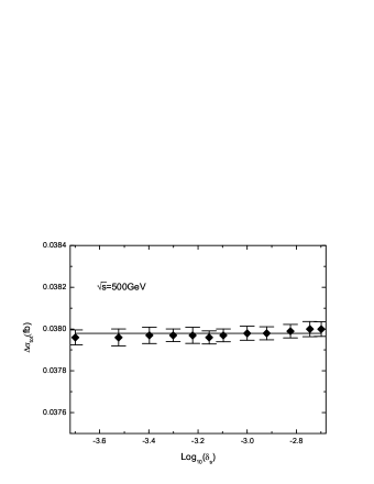
Figure 3: (a) The ${\cal O}(\alpha_{s})$ SQCD correction parts for cross section of $\gamma\gamma\to t\bar{t}Z^{0}$ process as the functions of the soft cutoff $\delta_{s}\equiv\Delta E_{g}/E_{b}$ in conditions of $m_{\tilde{g}}=200~{}GeV$, $m_{\tilde{t}_{1}}=147.59~{}GeV$, $m_{\tilde{t}_{2}}=337.34~{}GeV$, $\lambda=10^{-1}~{}GeV^{2}$ and $\sqrt{s}=500~{}GeV$. (b) The amplified curve marked with the calculation errors for $\Delta\sigma^{SQCD}$ of Fig.3(a) versus $\delta_{s}$.

In Fig.4(a) we present the LO, ${\cal O}(\alpha_{s})$ SQCD and SM-like QCD NLO corrected cross sections for the process $\gamma\gamma\to t\bar{t}Z^{0}$ with unpolarized and completely $+~{}+$, $+~{}-$ polarized photon beams, as the functions of colliding energy $\sqrt{s}$ in the conditions of $m_{\tilde{g}}=200~{}GeV$, $m_{\tilde{t}_{1}}=147.59~{}GeV$ and $m_{\tilde{t}_{2}}=337.34~{}GeV$. Their corresponding relative radiative corrections($\delta^{SQCD}\equiv\frac{\Delta\sigma^{SQCD}}{\sigma_{0}}$, $\delta^{SM-QCD}\equiv\frac{\Delta\sigma^{SM-QCD}}{\sigma_{0}}$) are shown in Fig.4(b). We can see from Figs.4(a-b) that the LO, SQCD and SM-like QCD corrected cross sections are sensitive to the colliding energy when $\sqrt{s}$ is less than $1~{}TeV$, while increase slowly when $\sqrt{s}>1.2~{}TeV$. Fig.4(b) shows that the SQCD and SM-like QCD relative radiative corrections have large values in the vicinity where the colliding energy is close to the $t\bar{t}Z^{0}$ threshold due to Coulomb singularity effect. We list some typical numerical results read from Figs.4(a,b) in Table 2. In considering the photon beam polarization, we introduce the conception of the polarization efficiency of photon beam, which is defined as $P_{\gamma}$($\equiv\frac{N_{+}-N_{-}}{N_{+}+N_{-}}$). We list the numerical results for $+~{}+$ and $+~{}-$ polarized photon collisions with $P_{\gamma}=1.0$ and $0.8$ in Table 2, respectively. From Fig.4(b) and Table 2 we can see clearly that the deviations of the NLO SQCD relative corrections from the corresponding SM QCD corrections in $+~{}+$ photon polarization collision mode, are much larger than in $+~{}-$ and unpolarized photon collision modes.

Figure 4: (a) The LO, SQCD and SM-like QCD one-loop corrected cross sections with $+~{}+$, $+~{}-$ polarized(with $P_{\gamma}=1.0$ ) and unpolarized photon beams for the process $\gamma\gamma\to t\bar{t}Z^{0}$ , as the functions of colliding energy $\sqrt{s}$ with $m_{\tilde{g}}=200~{}GeV$, $m_{\tilde{t}_{1}}=147.59~{}GeV$, $m_{\tilde{t}_{2}}=337.34~{}GeV$. (b) The corresponding relative radiative corrections in different polarization photon collision modes versus $\sqrt{s}$.

$\sqrt{s}(GeV)$	polarization	$\sigma_{0}(fb)$	$\sigma^{SM-QCD}(fb)$	$\sigma^{SQCD}(fb)$	$\delta^{SM-QCD}(\%)$	$\delta^{SQCD}(\%)$
	None	0.1181(1)	0.1615(1)	0.1560(1)	36.75(2)	32.09(2)
	$P_{\gamma}^{(++)}=1$	0.0799(1)	0.1082(2)	0.1027(1)	35.42(2)	28.53(2)
500	$P_{\gamma}^{(++)}=0.8$	0.0937(1)	0.1274(3)	0.1219(2)	35.97(3)	31.00(2)
	$P_{\gamma}^{(+-)}=1$	0.1564(1)	0.2150(2)	0.2095(2)	37.47(3)	33.95(2)
	$P_{\gamma}^{(+-)}=0.8$	0.1426(1)	0.1956(3)	0.1903(2)	37.17(3)	33.45(2)
	None	2.102(2)	2.244(5)	2.110(5)	6.76(4)	0.38(2)
	$P_{\gamma}^{(++)}=1$	1.468(2)	1.494(4)	1.345(4)	1.79(4)	-8.33(2)
800	$P_{\gamma}^{(++)}=0.8$	1.696(3)	1.763(5)	1.619(5)	3.95(5)	-4.54(3)
	$P_{\gamma}^{(+-)}=1$	2.737(3)	2.987(5)	2.869(5)	9.13(4)	4.82(2)
	$P_{\gamma}^{(+-)}=0.8$	2.509(3)	2.718(3)	2.595(5)	8.33(5)	3.43(3)

Table 2: Some typical numerical results of the LO, SQCD and SM-like QCD corrected cross sections in different polarized photon collision modes, which are obtained from Figs.4(a-b).

In Fig.5(a) we show the curves of the LO, SQCD and SM-like QCD NLO corrected cross sections for the process $\gamma\gamma\to t\bar{t}Z^{0}$ in unpolarized photon collision mode, as the functions of gluino mass with the colliding energy $\sqrt{s}=600~{}GeV$, the masses of scalar top-quarks $m_{\tilde{t}_{1}}=147.59~{}GeV$ and $m_{\tilde{t}_{2}}=337.34~{}GeV$. Their corresponding relative radiative corrections($\delta^{SQCD},\delta^{SM-QCD}$) as the functions of gluino mass are depicted in Fig.5(b). From these two figures we can see the pure SQCD NLO correction part always obviously counteracts the contribution from the SM-like NLO QCD correction in the whole plotted gluino mass range ($100~{}GeV<m_{\tilde{g}}<600~{}GeV$), especially when gluino has relative small mass value. We can see that in Fig.5(a) and Fig.5(b) there are negative peak structures at the vicinity of $m_{\tilde{g}}\sim 150~{}GeV$ respectively, where the mass values satisfy the relation $m_{\tilde{t}_{2}}\approx m_{\tilde{g}}+m_{t}$ and the resonance effect takes place.

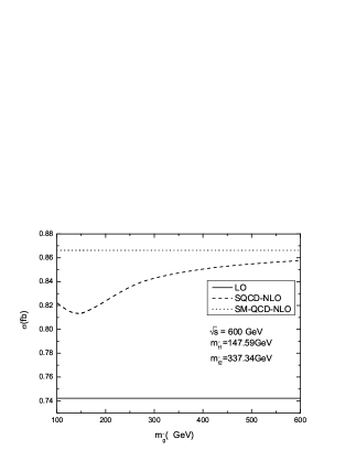
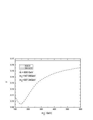
Figure 5: (a) The LO, SQCD and SM-like QCD one-loop corrected cross sections in unpolarized photon collision mode for the process $\gamma\gamma\to t\bar{t}Z^{0}$ , as the functions of gluino mass with $\sqrt{s}=600~{}GeV$, $m_{\tilde{t}_{1}}=147.59~{}GeV$ and $m_{\tilde{t}_{2}}=337.34~{}GeV$. (b) The corresponding relative radiative corrections of Fig.6(a) as the functions of gluino mass.

The LO, SQCD and SM-like QCD one-loop corrected cross sections for the process $\gamma\gamma\to t\bar{t}Z^{0}$ in unpolarized photon collision mode, as the functions of the lighter scalar top-quark mass $m_{\tilde{t}_{1}}$ are shown in Fig.6(a), and the corresponding relative radiative corrections($\delta^{SQCD}$, $\delta^{SM-QCD}$) as the functions of $m_{\tilde{t}_{1}}$ are presented in Fig.6(b). There we take $\sqrt{s}=600~{}GeV$, $m_{\tilde{g}}=200~{}GeV$ and $m_{\tilde{t}_{2}}=337.34~{}GeV$. Again these two figures show that the contribution from pure NLO SQCD correction partly cancels the NLO SM-like QCD correction when the $m_{\tilde{t}_{1}}$ varies in the range of [$100~{}GeV,~{}400~{}GeV$]. The cancellation becomes more significant when $m_{\tilde{t}_{1}}$ is less than $250~{}GeV$.

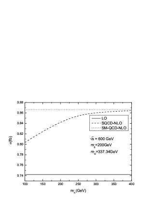
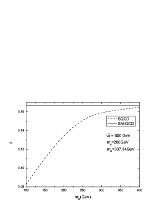
Figure 6: (a) The LO, SQCD and SM-like QCD one-loop corrected cross sections for the process $\gamma\gamma\to t\bar{t}Z^{0}$ in unpolarized photon collision mode, as the functions of scalar top-quark mass $m_{\tilde{t}_{1}}$ with $\sqrt{s}=600~{}GeV$, $m_{\tilde{g}}=200~{}GeV$ and $m_{\tilde{t}_{2}}=337.34~{}GeV$. (b) The corresponding relative radiative corrections of Fig.6(a) as the functions of $m_{\tilde{t}_{1}}$.

As we know that the distribution of transverse momentum of top-quark should be the same as that of anti-top-quark in the CP-conserving MSSM. Therefore, we shall not provide the distribution of $p_{T}^{\bar{t}}$ but only the $p_{T}^{t}$. We depict the differential cross sections of transverse momentum of top-quark at the LO, up to SQCD NLO and SM-like QCD NLO ($d\sigma_{0}/dp_{T}^{t}$, $d\sigma^{SQCD}/dp_{T}^{t}$ and $d\sigma^{SM-QCD}/dp_{T}^{t}$) in Fig.7(a), and the distributions of final $Z^{0}$-boson, $d\sigma_{0}/dp_{T}^{Z}$, $d\sigma^{SQCD}/dp_{T}^{Z}$ and $d\sigma^{SM-QCD}/dp_{T}^{Z}$, in Fig.7(b) separately, in the conditions of $\sqrt{s}=500~{}GeV$, $m_{\tilde{g}}=200~{}GeV$, $m_{\tilde{t}_{1}}=147.59~{}GeV$ and $m_{\tilde{t}_{2}}=337.34~{}GeV$. We can see from Figs.7(a-b) that in the plotted transverse momentum $p_{T}^{t}$($p_{T}^{Z}$) range, the LO differential cross section of $d\sigma_{0}/dp_{T}^{t}$($d\sigma_{0}/dp_{T}^{Z}$) is significantly enhanced by the NLO SM-like QCD and NLO SQCD corrections. The spectra of top-pair invariant mass, denoted as $M_{t\bar{t}}$, at the LO and up to NLO SM-like QCD and NLO SQCD are depicted in Fig.7 by taking $\sqrt{s}=500~{}GeV$, $m_{\tilde{g}}=200~{}GeV$, $m_{\tilde{t}_{1}}=147.59~{}GeV$ and $m_{\tilde{t}_{2}}=337.34~{}GeV$. We can see from the figure that when $M_{t\bar{t}}<400~{}GeV$ the NLO SM-like QCD and NLO SQCD corrections enhance the LO differential cross section $d\sigma_{LO}/dM_{t\bar{t}}$ obviously.

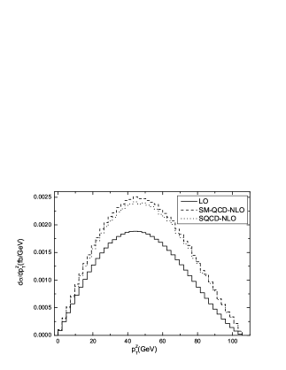
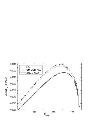
Figure 7: In the conditions of $\sqrt{s}=500~{}GeV$, $m_{\tilde{g}}=200~{}GeV$, $m_{\tilde{t}_{1}}=147.59~{}GeV$ and $m_{\tilde{t}_{2}}=337.34~{}GeV$, the LO, NLO SQCD and NLO SM-like QCD corrected differential cross sections of process $\gamma\gamma\to t\bar{t}Z^{0}$ in unpolarized photon collision mode. (a) The spectra of the transverse momentum of top-quark $p_{T}^{t}$. (b) The spectra of the transverse momentum of $Z^{0}$-boson $p_{T}^{Z}$. (c) The spectra of the invariant mass of top-quark pair $M_{t\bar{t}}$.

V. Summary

The future photon-photon collider would be an effective machine in probing precisely the SM and discovering the effects of new physics. In this paper, we have shown the phenomenological effects, due to the contribution from the NLO SQCD correction terms, can be demonstrated in the study of the top-pair production in association with a $Z^{0}$-boson via polarized and unpolarized photon-photon collisions. We discuss the relationships of the effects coming from the NLO SM-like QCD and complete NLO SQCD contributions to the cross section of process $\gamma\gamma\to t\bar{t}Z^{0}$ , with colliding energy $\sqrt{s}$, gluino mass $m_{\tilde{g}}$ and the lighter scalar top-quark mass $m_{\tilde{t}_{1}}$, separately. The LO, NLO SM-like QCD and complete NLO SQCD corrected spectra of the transverse momenta of final top-quark and $Z^{0}$-boson, and the differential cross section of final $t\bar{t}$-pair invariant mass are studied. We find that the pure SQCD correction to the cross section of process $\gamma\gamma\to t\bar{t}Z^{0}$ is sensitive to gluino and $\tilde{{t}_{1}}$ masses, and generally counteract the correction from the SM-like QCD NLO contributions. Our numerical results show that when $m_{\tilde{g}}=200~{}GeV$, $m_{\tilde{t}_{1}}=147.59~{}GeV$, $m_{\tilde{t}_{2}}=337.34~{}GeV$ and $\sqrt{s}$ goes up from $500~{}GeV$ to $1.5~{}TeV$, the relative NLO SQCD radiative correction to the cross section of the $\gamma\gamma\to t\bar{t}Z^{0}$ process in unpolarized photon collision mode, varies from $32.09\%$ to $-1.89\%$. And we find also the pure SUSY QCD NLO effects in $\gamma\gamma\to t\bar{t}Z^{0}$ process can be more significant in the $+~{}+$ polarized photon collision mode.

Acknowledgments: This work was supported in part by the National Natural Science Foundation of China(No.10575094, No.10875112), the National Science Fund for Fostering Talents in Basic Science(No.J0630319), Specialized Research Fund for the Doctoral Program of Higher Education(SRFDP)(No.20050358063) and a special fund sponsored by Chinese Academy of Sciences.

References

[1]
S. L. Glashow, Nucl. Phys. 22 (1961) 579; S. Weinberg, Phys. Rev. Lett. 1 (1967) 1264;
A. Salam, Proc. 8th Nobel Symposium Stockholm 1968,ed. N. Svartholm (Almquist and Wiksells, Stockholm 1968) p.367;
H. D. Politzer, Phys. Rep. 14 (1974) 129.
[2]
P. W. Higgs, Phys. Lett 12 (1964) 132, Phys. Rev. Lett. 13 (1964) 508;
Phys. Rev. 145 (1966) 1156; F. Englert and R.Brout, Phys. Rev. Lett. 13 (1964) 321;
G. S. Guralnik, C. R. Hagen and T. W. B. Kibble, Phys. Rev. Lett. 13 (1964) 585;
T. W. B. Kibble, Phys. Rev. 155 (1967) 1554.
[3] H.E. Haber and G. Kane, Phys. Rep. 117(1985)75; J.Gunion and H.E.
Haber, Nucl. Phys. B272, (1986)1.
[4]
W.M. Yao,et al. J. of Phys. G33,1 (2006).
[5]
Tevatron Electroweak Working Group(for the CDF and D0
Collaborations), Fermilab-TM-2347-E, TEVEWWG/top 2006/01, CDF-8162,
D0-5064, hep-ex/0603039v1.
[6]
F. Abe, et al. (CDF Collaboration), Phys. Rev. Lett. 74, 2626 (1995).
[7]
S. Abachi, et al. (DØ Collaboration), Phys. Rev. Lett. 74, 2632 (1995).
[8]
Zhou Mian-Lai, Ma Wen-Gan, Han Liang, Jiang Yi, Zhou Hong, Phys. Rev. D61 (2000)
033008; Zhou Mian-Lai, Ma Wen-Gan, Han Liang, Jiang Yi, Zhou Hong, J.Phys. G25 (1999)
27; A. Brandenburg, M. Maniatis, Phys. Lett. B558 (2003) 79.
[9]
C.F. Berger, M. Perelstein and F. Petriello, MADPH-05-1251, SLAC-PUB-11589,
arXiv:hep-ph/0512053; T. Abe et al. [American Linear Collider Working Group], in Proc of the APS/DPF/DPB Summer
Study on the Future of Particle Physics(Snowmass 2001) ed. N. Graf, arXiv:hep-ex/0106057.
[10]
R.S. Chivukula, S.B. Selipsky and E.H. Simmons, Phys. Rev. Lett. 69, 575 (1992);
R.S. Chivukula, E.H. Simmons and J. Terning, Phys. Lett. B331, 383 (1994);
K. Hagiwara and N. Kitazawa, Phys. Rev. D52, 5374 (1995); U. Mahanta,
Phys. Rev. D55, 5848 (1997) and Phys. Rev. D56, 402 (1997).
[11]
Parameters for Linear Collider, http://www.fnal.gov/directorate/icfa/LC_parameters.pdf
[12]
K. Hagiwara, H. Murayama and I. Watanabe, Nucl. Phys. B367(1991), 257.
[13]
Dai Lei, Ma Wen-Gan, Zhang Ren-You, Guo Lei, and Wang Shao-Ming,
Phys. Rev. D78 (2008) 094010, arXiv:0810.4365v1.
[15]
A. Denner, S. Dittmaier, M. Strobel, Phys. Rev. D53 (1996) 44.
[16]
T. Hahn, Comput. Phys. Commun. 140 (2001)418.
[17]
A. Denner, Fortschr. Phys. 41, 307 (1993).
[18]
T. Hahn, M. Perez-Victoria, Comput. Phys. Commun. 118
(1999)153.
[19]
G. J. van Oldenborgh, Phys Commun 66 (1991) 1, NIKHEF-H-90-15.
[20]
Zhang Ren-You, Ma Wen-Gan, Chen Hui, Sun Yan-Bin, and Hou Hong-Sheng,
Phys. Lett. B578(2004) 349.
[21]
Guo Lei, Ma Wen-Gan, Han Liang, Zhang Ren-You, and Jiang Yi, Phys. Lett. bf
B654 2007 13; Guo Lei, Ma Wen-Gan, Zhang Ren-You, and Wang Shao-Ming,
Phys. Lett. B662 2008 150
[22]
G. Passarino and M. Veltman, Nucl. Phys. B160, 151 (1979).
[23]
G.’t Hooft and M. Veltman, Nucl. Phys. B153 (1979) 365.
[24]
A. Denner, U Nierste and R Scharf, Nucl. Phys. B367 (1991)
637.
[25]
A. Denner and S. Dittmaier, Nucl. Phys. B658 (2003) 175.
[26]
B. W. Harris and J.F. Owens, Phys. Rev. D65 (2002) 094032,
arXiv:hep-ph/0102128.
[27]
A. Denner, Fortschr. Phys. 41, 307 (1993).
[28]
G. ’t Hooft and Veltman, Nucl. Phys. B153, 365 (1979).
[29]
W.M. Yao, et al., J. of Phys. G33,1 (2006).
[30]
F. Legerlehner, DESY 01-029, arXiv:hep-ph/0105283.
[31]
E. Boos, V. Bunichev, et al., (the CompHEP collaboration), Nucl.
Instrum. Meth. A534 (2004) 250-259, hep-ph/0403113.
[32]
T. Ishikawa,et al., (MINMI-TATEYA collaboration) ”GRACE
User’s manual version 2.0”, August 1, 1994.