Multimode quantum properties of a self-imaging OPO:
squeezed vacuum and EPR beams generation

Abstract

We investigate the spatial quantum properties of the light emitted by a perfectly spatially degenerate optical parametric oscillator (self-imaging OPO). We show that this device produces local squeezing for areas bigger than a coherence are that depends on the crystal length and pump width. Furthermore, it generates local EPR beams in the far field. We show, calculating the eigenmodes of the system, that it is highly multimode for realistic experimental parameters.

I Introduction

Highly multiplexed quantum channels are more and more needed as complexity increases in the quantum communication and information protocols. They can be obtained by coupling many single mode quantum channels Furosawa , but also by directly using highly multimode quantum systems. In addition, the resolution of several problems in quantum imaging book quantum imaging requires the generation of non-classical states of light having adjustable shapes in the transverse plane: this is the case for superresolution KolobovResolution , or for image processing below the standard quantum noise level trepsdelaubert . For all these reasons, it is very important to develop a source of highly multimode non classical light (squeezed and/or entangled) of arbitrary transverse shape.

In the continuous variable regime, where optical resonators are necessary to efficiently produce non-classical states, one of the keys to successfully generate multimode light is the ability to operate a multimode optical resonator. Indeed, many theoretical proposals rely on the use of an Optical Parametric Oscillator (OPO) operated below threshold with planar cavities kolobovlugiato95 or with confocal cavities Grangier Mancini Petsas which spatially filter half of the transverse modes. However, these proposals still did predict the arising of local vacuum squeezing and image amplification. Hence, we propose here to keep the parametric process to generate non-classical light but also to overcome the problems encountered by the use of a full transverse degenerate cavity : the self-imaging cavity Arnaud . This type of resonator, used for instance to improve the power of multimode lasers Couderc , is in principle able to transmit any optical image within its spatial bandwidth.

The aim of this article is to demonstrate that the self-imaging OPO is an excellent candidate to produce local squeezing, image amplification and also local EPR beams, taking into account its physical limitations such as the thickness of the crystal and the finite size of the various optical beams and detectors.

The following section (section II) describes the experimental configuration and develops the theoretical model, as well as the method used to determine the squeezing spectra measured in well-defined homodyne detection schemes. In section III, the results for such quantities respectively in the near field and in the far field are given, and we investigate the generation of EPR beams. Finally, in section IV we compute the eigenmodes of the system and show that they are closed to Hermite Gauss modes.

II Self-imaging Optical Parametric Oscillator

II.1 The self-imaging cavity

We consider the parametric down conversion taking place in a self-imaging optical parametric oscillator whose cavity has been depicted in the pioneer article of $Arnaud$ Arnaud . Such a cavity is a fully transverse degenerate one, which implies that all the transverse modes of same frequency resonate for the same cavity length. From a geometrical point of view an optical cavity is self imaging when an arbitrary ray retraces its own path after a single round trip. In such a cavity, in the paraxial approximation, the $ABCD$ matrix $M$ after one round trip is equal to identity:

$$\begin{pmatrix}A&B\\ C&D\end{pmatrix}=\begin{pmatrix}1&0\\ 0&1\end{pmatrix}$$ (1)

The simplest self imaging ring cavity requires three lenses of focal length $f_{i}$, $i=1,2,3$ (Arnaud ). As depicted in Fig(1), the ring cavity is self-imaging provided the distances $c_{ij}$ of the image plane of the lens $i$ and the objet plane of the lens $j$ are given by:

$$c_{12}=\frac{f_{1}f_{2}}{f_{3}},\\ c_{23}=\frac{f_{2}f_{3}}{f_{1}},\\ c_{31}=\frac{f_{3}f_{1}}{f_{2}}$$ (2)

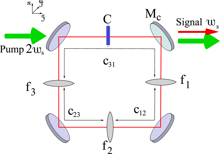
Figure 1: Self-imaging OPO scheme in a ring cavity configuration

Let us consider an Optical Parametric Oscillator (OPO) whose cavity is the self-imaging one described in Fig.1 (Mancini ). A type I parametric medium of length $l_{c}$ is centered on the plane C located at the longitudinal coordinate z=0. The OPO is pumped by a gaussian $TEM_{00}$ field $E_{p}$ of amplitude $A_{p}$ and frequency $\omega_{p}=2\omega_{s}$. Its waist $w_{p}$ is located at the plane C. The OPO works in a longitudinal degenerate operation for which signal and idler have the same frequency $\omega_{s}$. We assume that for the pump wave, all the mirrors are totally transparent, and that for the signal field, the coupling mirror $M_{c}$ has a small transmission $t$, the other three mirrors being perfectly reflecting.

II.2 Electric field operators

We will follow an operational approach GattiLugiato close to the one developed in the confocal case Lopez , and in order to keep the present article concise we give only the main steps of the calculation. The intracavity signal field at frequency $\omega_{s}$ is described by a field envelope operator ${B}(\textbf{x},z)$. In the self imaging resonator, at resonance, the field can be decomposed on any transverse mode basis (such as the Gauss-Laguerre modes for instance). The field operator becomes :

$${B}(\textbf{x},z,t)=\sum_{l}f_{l}(\textbf{x},z){a}_{l}(z,t)\,,$$ (3)

where ${a}_{l}(z,t)$ is the annihilation operator of a photon in mode $l$ at the cavity position $z$ and at time $t$. $f_{l}$ is the amplitude of the $l$ mode. This field obeys the standard equal time commutation relation at a given transverse plane at position $z$:

$$[{B}(\textbf{x},z,t),{B}^{\dagger}(\textbf{x'},z,t)]=\delta(\textbf{x}-\textbf{x'}).$$ (4)

Indeed, contrary to the confocal case Lopez or to any partially imaging cavity case, this operator is the same as the one in the vacuum as no spatial filtering is induced by the cavity. In the regime below threshold considered here, the pump is not depleted, and fluctuations of the pump field do not contribute, at first order to the fluctuations of the signal.

The interaction Hamiltonian of the system, taking into account the thickness of the crystal and the shape of the pump, is given by

$$H_{int} = \frac{i\hbar g}{2l_{c}}\int_{-l_{c}/2}^{l_{c}/2}dz^{\prime}\int\int d^{2}x^{\prime}\{A_{P}(\textbf{x'},z^{\prime})[{B^{\dagger}}(\textbf{x'},z^{\prime},t)]^{2}$$ (5)

$$-h.c.\}\,,$$

where g is the coupling constant proportional to the second order nonlinear susceptibility $\chi^{(2)}$.

II.3 Evolution equation of the field

In this section, we investigate the intracavity evolutions of the signal field in the crystal plane C (near field) and of its spatial fourier transform (far field), taking into account the crystal thickness and the finite size of the pump. The nonlinear interaction is supposed to be very weak, so that the field amplitude in a single pass through the crystal is only slightly affected. Therefore, the $z$ dependence of the operators ${a}_{l}$ can be removed in Eq(5). The longitudinal variation of the signal operator ${B}$ is due to the diffraction described in the modal functions $f_{l}(\textbf{x},z)$.

II.3.1 Near-field evolution

At the mid-point plane $z=0$ of the crystal, designated as the near field plane in the following, the ${B}$ field evolution can be expressed as the sum of a damping and free propagation term inside the cavity and of a parametric interaction term :

$$\frac{\partial{B}}{\partial t}(\textbf{x},0,t)=-\gamma(1+i\delta){B}(\textbf{x},0,t)$$ (6)

$$+g\int\int d^{2}x"K_{int}(\textbf{x},\textbf{x"}){B}^{\dagger}(\textbf{x"},0,t)+\sqrt{2\gamma}{B}_{in}(\textbf{x},0,t)$$

where $\gamma$ is the cavity escape rate, $\delta$ the normalized cavity detuning of the modes, and ${B}_{in}$ the input field operator. $K_{int}$ is the integral kernel describing the non-linear interaction. Assuming exact collinear phase matching $k_{p}=2k_{s}$, and neglecting walk off, this kernel associates two points x and x” through the pump amplitude at the average position $\frac{\textbf{x}+\textbf{x"}}{2}$, and a function $\Delta(\textbf{x}-\textbf{x"})$ describing the diffraction effects within the crystal.

$$K_{int}(\textbf{x},\textbf{x"}) = A_{p}(\frac{\textbf{x}+\textbf{x"}}{2})\Delta(\textbf{x}-\textbf{x"})$$ (7)

with

$$\Delta(\textbf{x}-\textbf{x"})=\frac{ik_{s}}{4\pi l_{c}}\int_{-l_{c}/2}^{l_{c}/2}\frac{dz^{\prime}}{z^{\prime}}e^{\frac{ik_{s}}{4z^{\prime}}|\textbf{x}-\textbf{x"}|^{2}}$$ (8)

where $k_{s}=n_{s}\omega_{s}/c$ is the field wavenumber, and $n_{s}$ the index of refraction at frequency $\omega_{s}$. It can be expressed in terms of the integral sine function $Si(x)=\int_{0}^{x}\frac{\sin udu}{u}$

$$\Delta(\textbf{x}-\textbf{x"})=\frac{k_{s}}{2\pi l_{c}}\left(\frac{\pi}{2}-Si(\frac{k_{s}|\textbf{x}-\textbf{x"}|^{2}}{2l_{c}})\right).$$ (9)

In the thin crystal case ($l_{c}\rightarrow 0$) the function $\Delta(\textbf{x}\pm\textbf{x"})$ tends to the usual two-dimensional distribution $\delta(\textbf{x}\pm\textbf{x"}$.

In the thick crystal case, the parametric interaction mixes the operators at different points of the transverse plane, over areas of finite extension given by the spatial extension of the kernel $K_{int}$. This extension is characterized by the width of the sine function, which define a coherence length :

$$l_{coh}=\sqrt{\frac{\lambda l_{c}}{\pi n_{s}}}.$$ (10)

When $|\textbf{x}-\textbf{x"}|\gg l_{coh}$, $\Delta$ and therefore the kernel $K_{int}$ take negligible values, there is no coupling between these two positions. On the other hand, when $|\textbf{x}-\textbf{x"}|\ll l_{coh}$ the coupling mixes the fluctuations. Thus, we can define $l_{coh}$ as the quantum resolution of our system.

Because of the finite size of the pump, the kernel will take negligible values for $\textbf{x}+\textbf{x"}>w_{p}$. Therefore, we can define the number of transverse modes excited by the parametric process inside the cavity, as the ratio between the size of the pump, and the area defined by $l_{coh}$.

$$b=\frac{w_{p}^{2}}{l_{coh}^{2}}$$ (11)

This definition relies on the classical imaging properties of the system. We will show in the last section of this article show that it is consistent with the computation of the eigenmodes of the system.

II.3.2 Far-field evolution

Let us introduce the spatial Fourier transform of the signal field envelope operator (Lopez )

$$\tilde{B}(\textbf{q},z,t) = \int\frac{d^{2}x}{2\pi}{B}(\textbf{x},z,t)e^{-i\textbf{q}\cdot\textbf{x}}$$ (12)

Equation (6) becomes:

$$\frac{\partial\tilde{B}}{\partial t}(\textbf{q},0,t)=-\gamma(1+i\Delta)\tilde{B}(\textbf{q},0,t)+$$ (13)

$$g\int d^{2}q"\tilde{K}_{int}(\textbf{q},\textbf{q"}){B}^{\dagger}(\textbf{q"},0,t)+\sqrt{2\gamma}\tilde{B}_{in}(\textbf{q},0,t)\,,$$

where the coupling Kernel $\tilde{K}_{int}(\textbf{q},\textbf{q"})$ is the Fourier transform of the kernel (7) with respect to both arguments. Straightforward calculations show that

$$\tilde{K}_{int}(\textbf{q},\textbf{q'}) = \tilde{A_{p}}(\textbf{q}+\textbf{q'}){\rm sinc}[\frac{l_{c}}{2k_{s}}|\frac{\textbf{q}-\textbf{q'}}{2}|^{2}]$$ (14)

where $\tilde{A_{p}}$ is the spatial Fourier transform of the Gaussian pump profile, i.e. $\tilde{A}_{p}(\textbf{q})=\frac{w_{p}^{2}}{2}A_{p}\exp{(-|\textbf{q}|^{2}\frac{w_{p}^{2}}{4})}$.

The sinc term in the coupling kernel of Eq. (14) is the Fourier transform of the $\Delta$ terms in Eq. (7)), and correspond to the limited phase-matching bandwidth of the nonlinear crystal. For a thin crystal, phase matching is irrelevant and there is no limitation in the spatial bandwidth of down-converted modes, whereas for a thick crystal, the cone of parametric fluorescence has an aperture limited to a bandwidth of transverse wavevectors $\Delta q\approx 1/l_{coh}\propto 1/\sqrt{\lambda l_{c}}$. In the self imaging geometry, the cavity ideally transmits all the Fourier modes, so that the spatial bandwidth is only limited by the phase matching along the crystal. Finally, we have to notice that in the far field configuration the $\tilde{A_{p}}(\textbf{q}+\textbf{q'})$ couples different q-vectors modes within the finite width of the pump.

II.4 Input/output relation

In order to calculate the noise spectrum of the outgoing field, an input/output method is used. The input field is supposed to be in a coherent state and the fluctuations at the output can be inferred. The relation linking the outgoing fields $B^{out}(\textbf{x},t)$ to the intracavity and input fields at the cavity input/output portGardiner is:

$$B^{out}(\textbf{x},t)=\sqrt{2\gamma}B(\textbf{x},t)-B^{in}(\textbf{x},t)$$ (15)

The evolution equation of the field, either in the near or in the far field can be solved in the frequency domain by introducing:

$$B^{in/out}(\textbf{x},\Omega)=\int\frac{dt}{\sqrt{2\pi}}B^{in/out}(\textbf{x},t)e^{-i\Omega t}$$

which lead to the input/output relation, linking $B^{in}(\textbf{x},\Omega)$ and $B^{out}(\textbf{x},\Omega)$.

In the case of a thin crystal in the near fieldPetsas , this relation describes an infinite set of independent optical parametric oscillators. In this case the squeezing spectrum can be calculated analytically. More generally, this relation in near field links all points in the transverse plane within the coherence area. In order to get the input/output relation, we have to inverse the input/output relation by using a numerical method used in Lopez .

II.5 Homodyne detection scheme in the near field and far field

In the following sections we calculate the noise spectrum at the output of the OPO as a function of the detected transverse mode selected by an homodyne detection scheme homodynespatiale . By mixing it with a coherent Local Oscillator (LO) of various shape on a 50% beamsplitter (reflection and transmission coefficients $\textit{r}=\frac{1}{\sqrt{2}}$ and $\textit{t}=\frac{1}{\sqrt{2}}$), one can measure the fluctuations on any transverse mode of the output of the self imaging OPO, by measuring the photocurrents difference. The two identical detectors of different size and position are supposed to have a perfect quantum efficiency. All the fields are evaluated at the beam-splitter location, and the z-dependence is omitted in the following.

We use two different configurations : near-field (x-position basis) and far-field (q-vector basis). The complete detection scheme is schematically shown in Fig. 2 and 3. In the near-field configuration, the imaging scheme is composed of a two-lens afocal system (focal length f) which images the crystal/cavity center plane C onto the detection planes D and D’(near field planes). In the far field configuration, a single lens of focal length f transforms its focal object plane C into the image focal detection plane D. Any image in the object plane C is tranformed into its fourier transform in the plane D (far field plane).

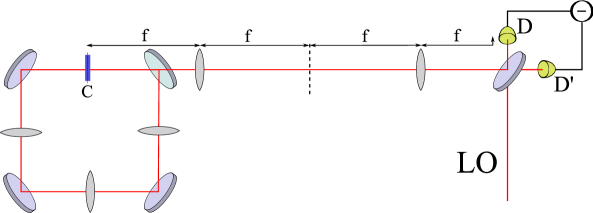
Figure 2: Balanced homodyne detection scheme in the near field. Two matching lenses of focal f are used to image the cavity center C at the detection planes D and D’

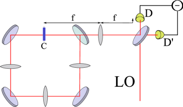
Figure 3: Balanced homodyne detection scheme in the far field. A matching lens of focal f is used to obtain the far field image of the object plane C at the detection planes D and D’

For near-field imaging, the local oscillator can be expressed as $\alpha_{L}(\textbf{x},z)=|\alpha_{L}(\textbf{x},z)|e^{i\varphi_{L}(\textbf{x},z)}$. The difference photocurrent is a measure of the quadrature operator:

$$E_{H}(\Omega)=\!\!\!\!\int_{det}\!\!\!\!d\textbf{x}\left[B^{out}(\textbf{x},\Omega)\alpha_{L}^{*}(\textbf{x})+B^{out+}(\textbf{x},-\Omega)\alpha_{L}(\textbf{x})\right]\,$$ (16)

where det is the image of the photodetection region at the crystal plane C, and assumed to be identical for the two photodetectors. The quantum efficiency of the photodetector is assumed to be equal

For far-field imaging, the lens provides a spatial Fourier transform of the output field $B_{out}(x,\Omega)$, so that at the location of plane D the field $B^{out}_{D}(x,\Omega)$ is:

$$B^{out}_{D}(x,\Omega)=\frac{2\pi}{\lambda f}\tilde{B}^{out}(\frac{2\pi}{\lambda f}x,\Omega)$$ (17)

In this plane, $B^{out}_{D}(x,\Omega)$ is mixed with an intense stationary and coherent beam $\alpha_{LO}^{D}(x)=\frac{2\pi}{\lambda f}\tilde{\alpha}_{LO}(\frac{2\pi x}{\lambda f},\Omega)$, where $\alpha_{L}(x)$ has a gaussian shape, with a waist $w_{LO}$. The homodyne field has thus an expression similar to the near field case, where functions of $x$ are now replaced by their spatial Fourier transforms:

$$E_{H}(\Omega)=$$ (18)

$$\int_{det}d\textbf{q}[\tilde{B}^{out}(\textbf{q},\Omega)\tilde{\alpha}_{LO}^{*}(\textbf{q})+\tilde{B}^{out+}(\textbf{q},-\Omega)\tilde{\alpha}_{LO}(\textbf{q})]$$

In near- and far-field, the fluctuations $\delta E_{H}(\Omega)$ of the homodyne field around steady state are characterized by a noise spectrum:

$$V(\Omega)=\int_{-\infty}^{+\infty}d\Omega^{\prime}\langle\delta E_{H}(\Omega)\delta E_{H}(\Omega^{\prime})\rangle=N+S(\Omega)$$ (19)

where $E_{H}$ is normalized so that $N$ gives the mean photon number measured by the detector

$$N=\int_{det}d\textbf{x}|\alpha_{L}(x)|^{2}$$ (20)

N represents the shot-noise level, and S is the normally ordered part of the fluctuation spectrum, which accounts for the excess or decrease of noise with respect to the standard quantum level (S=0). One should note that there is a complete equivalence between a setup with a finite and flat local oscillator and infinite detectors, and a flat and infinite local oscillator combine with finite size detectors. We will often use the configuration with finite size photodetectors in the following.

III Non-classical properties

We expose here the main properties of the fields emitted by the sub-threshold self-imaging OPO. We will first consider the squeezing in the near-field in a very similar manner as what was done for a confocal OPO. Then we will study the far field properties and demonstrate local EPR correlations.

III.1 Squeezing in the near field

As the self imaging cavity does not exert any spatial filtering on the fields, the non-classical properties are very similar to those observed in the single pass configuration. We will here show the main squeezing predictions for such a device, taking into account the thickness of the crystal. The corresponding calculations are avalaible upon request to the authors.

Let us first consider the case of the thin crystal approximation, where no characteristic length is introduced in the model. We consider a thin crystal self-imaging OPO pumped by a gaussian beam. We look at the output quantum fluctuations with a pixel-like detector whose position is varied. In figure 4, the squeezing is plotted as a function of the detector distance from the optical axis for different mean powers of the pump ($A_{p}=1$ corresponding to the threshold on the axis). The squeezing is maximum when the detection is centered on the pump beam, and tends to zero far from the center. Figure 4 shows that the squeezing increases with the total pump power and depends critically on its local value. Hence, any transverse position on the crystal acts as an independent OPO.

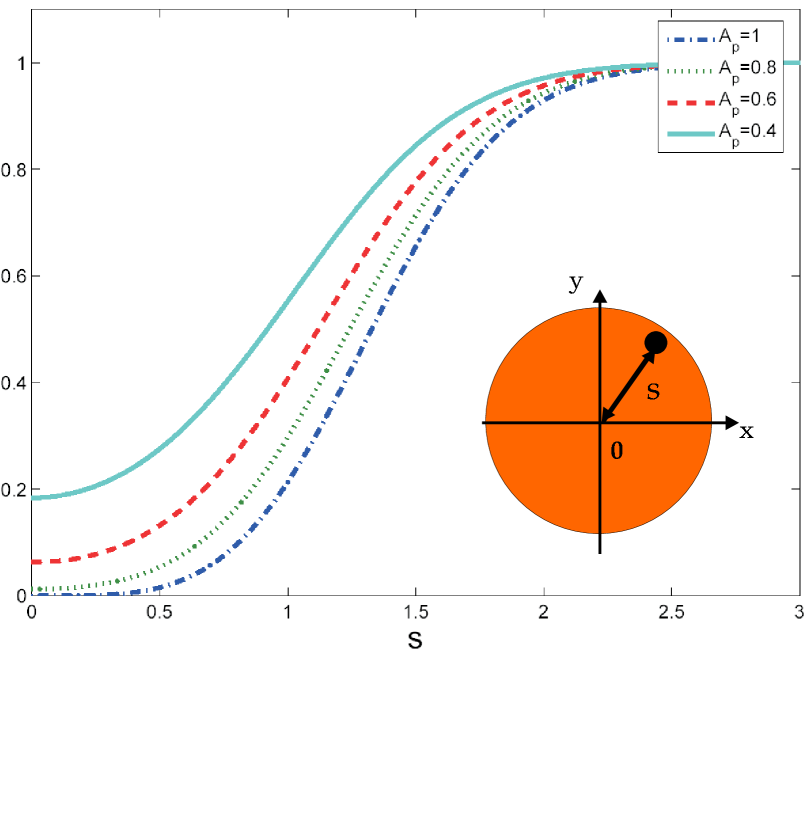
Figure 4: Quantum noise at zero-frequency normalized to the shot noise, for a pixel like detector located in the near field plane, as a function of the pixel distance from the origin $s$, normalized to the waist of the pump ($s=\frac{\rho}{w_{p}}$) and for different pump values

The same behavior is observed in a configuration closer to actual experimental scheme using a circular detector whose radius $\Delta\rho$ can be varied. Like in the previous case, the curves in figure 5 are crucially dependent on the pump power.

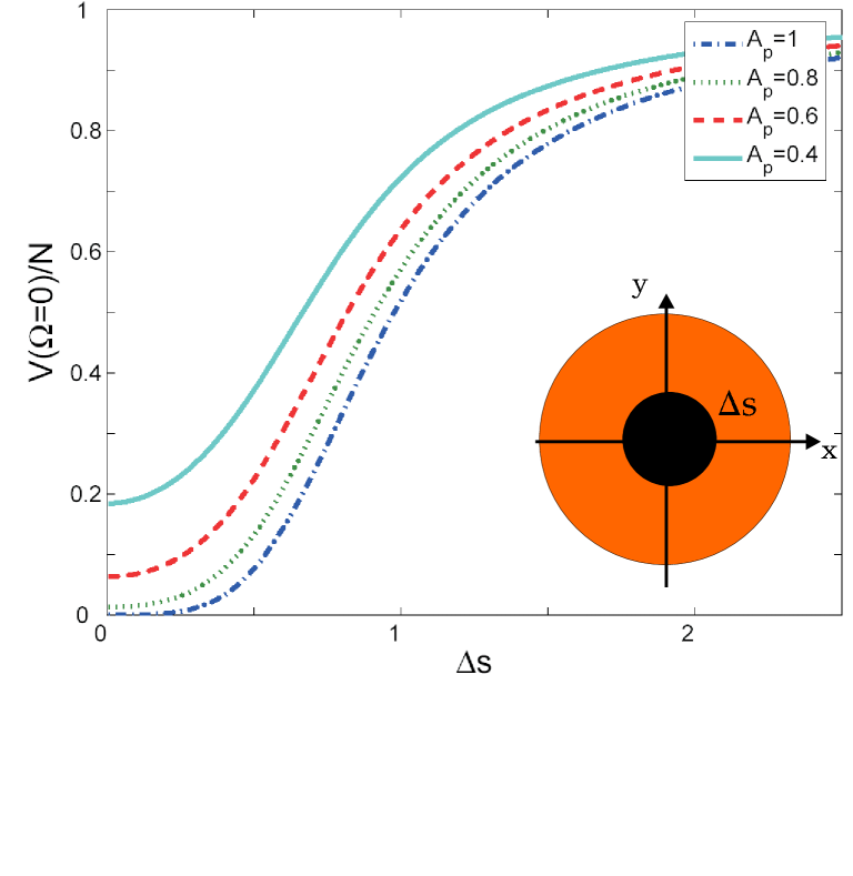
Figure 5: Quantum noise at zero-frequency, normalized to the shot noise, in the thin crystal case, for a circular detector in the near field plane, as a function of the radius of the detector normalized to the pump waist $\Delta s=\frac{\Delta\rho}{\omega_{p}}$

In a more general realistic study, we have to take into account the finite size of the crystal. For a thick crystal, the coherence length $l_{coh}$ introduced in equation (10) has to be taken into account. On transverse size smaller than this coherence length, fluctuations are mixed inside the crystal.
In a first step, we consider a quasi plane pump for which its waist $w_{p}$, considered as infinite, is much larger than the coherence area and can excite many modes. The detector is centered with respect to the optical axis and its size can be changed. As shown in figure 6, the squeezing is maximum when its size is larger than the coherence area, and the noise tends to shot noise for a pixel like detector, whose size becomes smaller than the coherence length. At the scale of the coherence area, the OPO can be considered as locally single mode and the local fluctuations are mixed. In regions smaller than the coherence area independent modes having their own fluctuations cannot be excited. For large detectors, several coherence area can be excited, the OPO can be considered as multimode, and the squeezing is maximum. The coherence length sets the limit between single mode and multimode operation.
In a second step, we have to consider a more realistic case for which the pump waist $w_{p}$ is finite. In figure 7, we represent the quantum noise as a function of the detector size for different pump waist (normalized to the coherence length). For detectors smaller than the coherence area, the quantum noise goes to shot noise whatever the size of the pump is. As explained in the last paragraph, at that scale the OPO can be considered as locally single mode and no squeezing can be obtained. For detectors whose size is close the coherence area one, squeezing is obtained. Nevertheless this squeezing degrades for a given pump waist when the size of the detector increases. For a given pump size, when the detector becomes larger than the excited surface, vacuum fluctuations are coupled to the detected signal and the squeezing degrades. In the same way, for a given detector size, the squeezing decreases with the waist of the pump. In fact a finite pump size limits the number of excited modes. Increasing the pump size, increase the number of excited modes and improve the squeezing.

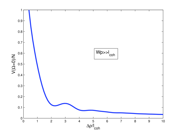
Figure 6: Quantum noise at zero-frequency, normalized to the shot noise, in the thick crystal case, as a function of the detector radius (scaled to $l_{coh}$).The detector in centered on the pump beam

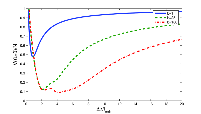
Figure 7: Quantum noise at zero-frequency, normalised to the shot noise, in the thick crystal case, as a function of the radial size of the detector scaled to $l_{coh}$, plotted for several values of the parameter $b=\frac{{w_{p}}^{2}}{{l_{c}oh}^{2}}$

III.2 Entanglement in the far field

In the far field, the analysis has to be performed not in crystal plane (near field plane) but in its Fourier plane (far field plane). Squeezing can be observed in the far field when using a symmetric detector. Indeed, contrary to the near-field case, in the far field configuration the down conversion process couples two symmetric $k$ vectors. Thus in order to recover the squeezing one needs a symmetric detector relative to the optical axis of the imaging system. The results obtained are therefore the same as those in the confocal cavity, both with a plane pump and with a finite pump. Corresponding calculations are also available upon request to the authors.

The advantage of the self imaging cavity is that it does not couple the two symmetrical $k$ vectors. Therefore one expects correlations between two symmetrical areas in the far field, as it will be shown in the following.

In order to characterize the correlation level between symmetrical parts of the beam, we compare the quadrature field fluctuations on two symmetrical pixels. In order to get this quantities, we use the homodyne detection scheme (figure 8) proposed in homodynespatiale , where two symmetrical sets of two detectors measure a quadrature of the field at two symmetrical positions.

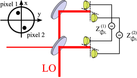
Figure 8: Homodyne detection scheme for the measurement of the quadrature components of the output field on two symmetrical pixels: pixel 1 and pixel 2

Let us consider a pixel-like detector with finite detection area $\Delta\rho_{j}$, according to equation 18 the detected field quadrature is given by :

$$E_{\phi_{L}}^{(j)}(\Omega) = \int_{\Delta\rho_{j}}\!\!\!\!\!\!d\textbf{q}\left[\tilde{B}^{out}(\textbf{q},\Omega)|\alpha_{L}(\textbf{q})|e^{-i\phi_{L}}+\right.$$ (21)

$$\left.\tilde{B}^{out+}(\textbf{q},-\Omega)|\alpha_{L}(\textbf{q})|e^{i\phi_{L}}\right]$$

where we have introduced explicitly the phase of the local oscillator. To compare the fluctuations of the field quadrature measured in two symmetrical pixels $j=1$ and $j=2$, we compare the sum and the difference of these quantities.

$$E_{\phi_{L}}^{(\pm)}(\Omega)=E_{\phi_{L}}^{(1)}(\Omega)\pm E_{\phi_{L}}^{(2)}(\Omega)$$ (22)

In order to evaluate the degree of correlation or anti-correlation, we introduce the corresponding fluctuations spectra:

$$V_{\phi_{L}}^{(\pm)}(\Omega)=\int_{-\infty}^{+\infty}d\Omega^{\prime}\langle E_{\phi_{L}}^{(\pm)}(\Omega)E_{\phi_{L}}^{(\pm)}(\Omega^{\prime})\rangle$$ (23)

Straightforward calculations show that:

$$V_{\phi_{L}}^{(-)}(\Omega)=V_{\phi_{L}+\pi/2}^{(+)}(\Omega)$$ (24)

It results that the correlation between $E_{\phi_{L}}^{(1)}$ and $E_{\phi_{L}}^{(2)}$ is the same that the anticorrelation between the corresponding orthogonal quadrature components $E_{\phi_{L}+\pi/2}^{(1)}$and$E_{\phi_{L}+\pi/2}^{(2)}$. In order to calculate (23), we develop the expression, so as:

$$V_{\phi_{L}}^{(\pm)}(\Omega) = \int_{-\infty}^{+\infty}d\Omega^{\prime}\langle E_{\phi_{L}}^{(1)}(\Omega)E_{\phi_{L}}^{(1)}(\Omega^{\prime})\rangle$$ (25)

$$+\int_{-\infty}^{+\infty}d\Omega^{\prime}\langle E_{\phi_{L}}^{(2)}(\Omega)E_{\phi_{L}}^{(2)}(\Omega^{\prime})\rangle$$

$$\pm\int_{-\infty}^{+\infty}d\Omega^{\prime}\langle E_{\phi_{L}}^{(1)}(\Omega)E_{\phi_{L}}^{(2)}(\Omega^{\prime})\rangle$$

$$\pm\int_{-\infty}^{+\infty}d\Omega^{\prime}\langle E_{\phi_{L}}^{(2)}(\Omega)E_{\phi_{L}}^{(1)}(\Omega^{\prime})\rangle$$

The terms $\int_{-\infty}^{+\infty}d\Omega^{\prime}\langle E_{\phi_{L}}^{(i)}(\Omega)E_{\phi_{L}}^{(i)}(\Omega^{\prime})\rangle$ correspond to the result of the fluctuation spectra of a homodyne detection scheme using a single pixel. The other terms are cross correlation terms, so that:

$$V_{\phi_{L}}^{-}(\Omega)=V_{\phi_{L}+\pi/2}^{+}(\Omega)$$ (26)

When these variances are bellow one, EPR beams are obtained at the output of the self-imaging cavity. One should note that these variances correspond to the fluctuation spectrum obtained performing a homodyne detection in the far field with symmetric detectors : the usual connection between squeezing and quantum correlations is exhibited, both side of the same phenomenonQuantim . More specifically, the spatial entanglement in the far field arise from the correlations between the modes ${a}_{\textbf{q}}\sim e^{i\textbf{q.x}}$ and ${a}_{-\textbf{q}}\sim e^{-i\textbf{q.x}}$. As ${a}_{\textbf{q}}$ and ${a}_{-\textbf{q}}$ are EPR entangled beams, it is well know that the combination of modes:

$$\frac{{a}_{\textbf{q}}+{a}_{-\textbf{q}}}{\sqrt{2}}\sim\cos(\textbf{q.x})$$

$$\frac{{a}_{\textbf{q}}-{a}_{-\textbf{q}}}{\sqrt{2}}\sim\sin(\textbf{q.x})$$ (27)

will be squeezed with respect to two orthogonal quadrature components. The modes proportional to $\cos(\textbf{q.x})$ are the even modes: using an even detection scheme it is possible to see squeezing, as already found in the previous section. Note that if we use an odd detection scheme (symmetrical detectors with an odd local oscillator), it will be also possible to see squeezing in the far field, but on the orthogonal quadrature.

In order to ascertain the inseparable character of this physical state, Duan et al.Duan have shown one needs to make two joint correlation measurements on non commuting observables on the system. They have shown that in the case of gaussian states there exists a criterion of separability in terms of the quantity $S_{12}$, that we will call ’separability’, and is given by:

$$S_{12}(\Omega)=\frac{1}{2}(V_{\phi_{L}}^{-}(\Omega)+V_{\phi_{L}+\frac{\pi}{2}}^{+}(\Omega))$$ (28)

The suddicient Duan criterion for inseparability is given by:

$$S_{12}(\Omega)<1$$ (29)

First, we can perform a joint correlation measurement using two split detectors of same but variable size as depicted in Figure 9. Figure 10 shows the evolution of the separability at zero frequency $S_{12}(0)=S_{12}$ for different b parameters, in function of the detector radius scaled to $l_{cohf}=\lambda f/2\pi w_{p}$ Lopez . Notice that results are the same as a local squeezing measurement using a circular detector of variable radius $\Delta\rho$ centered on the optical axis.

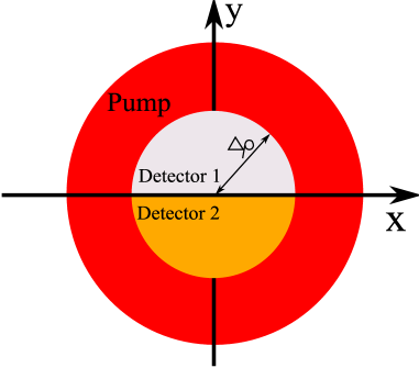
Figure 9: Detection scheme for the inseparability measurement

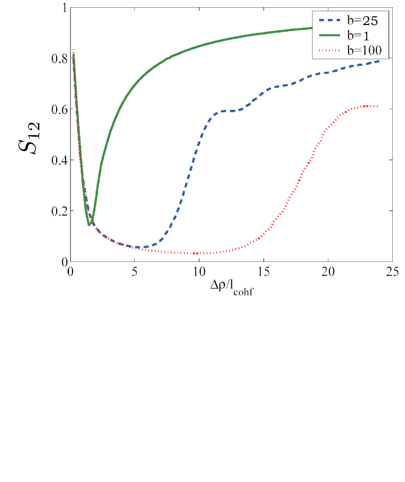
Figure 10: Inseparability at zero-frequency, and at resonance, as a function of the radial amplitude of the detector $\Delta\rho$(scaled to the coherence area $l_{cohf}$) , in the finite pump regime and far field approach and for different values of b.

Fig. 11 shows the results obtained in the case of two symmetrical pixels (pixel of size equal to the coherence length $l_{cohf}$, for different b values, in function of the distance between the two pixels $\rho$.

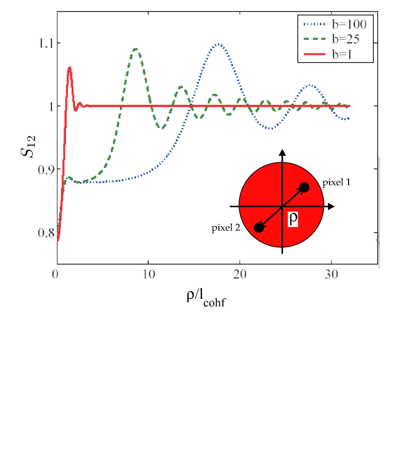
Figure 11: Inseparability at zero-frequency, and at resonance, as a function of the distance between the two pixels $\rho$ (scaled to the coherence area $l_{cohf}$, in the finite pump regime and far field approach and for different values of b.

IV Pixel-based model for the self-imaging OPO

We have so far described the non-classical properties of the self-imaging OPO using detection based geometry, very appropriate to describe actual experiments. However, it is known that any input/output system can be described by eigenmodes : for instance in the case of mode-locked pulses of light incident on a non-linear cristal, it has been shown that independent modes could be found, either using the Schmidt decomposition in the single photon regime Walmsley or diagonalising the coupling matrix in the continuous wave regime Patera . We propose here to use the same technique to exhibit the eigenmodes of the system and give a more precise value of the number of modes involved in the process.

Let us pixelize the transverse space with pixels much smaller than $l_{coh}$ and develop the OPO equations onto the pixel operators. To simplify the system, we can first consider a one dimension pixelization. Let $L$ be the size of the pixelized zone, and $N$ the number of pixels. The pixel $i$ is defined as the zone of size $\frac{L}{N}$ near the abscissa $x_{i}=i\frac{L}{N}$, with i ranging from $-N/2$ to $N/2$. The pixel operator is therefore :

$$B_{i}=\int_{S_{i}}dxB(x)$$ (30)

The pixel size must be chosen small enough to ensure the constant value of $A_{p}$ and $K_{int}$ on every pixel. In this case, the Kernel can be written as :

$$K_{int}(i,j)=K_{int}(\textbf{x}_{i},\textbf{x}_{j})$$ (31)

and the evolution equation (6) at zero frequency then becomes :

$$-\gamma{B}_{i}+\frac{gL}{N}\sum_{j}K_{int}(i,j){B}^{\dagger}_{j}+\sqrt{2\gamma}{B}^{in}_{i}=0$$ (32)

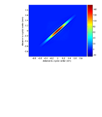
(a)

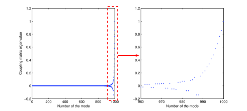
(b)

Figure 12: a) Coupling Matrix $K_{int}$ between two points of the crystal b) Spectrum of this matrix.

To solve these N coupled equations, one must find the eigenvectors and eigenvalues of the matrix $K_{int}(i,j)$. The K matrix and its spectrum are represented on figure 12. Its diagonalization gives a set of eigenmodes with corresponding eigenvalues. Some of these eigenmodes are represented on figure 13, they are very close to Hermite-Gauss polynomials shapes whose characteristic waist is imposed, in our case, by the pump waist.

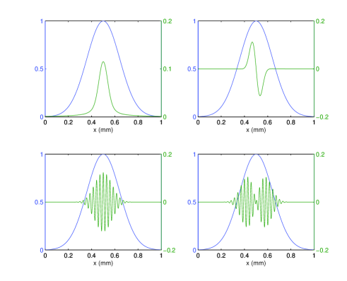
Figure 13: Shape of the eigenvectors of matrix $K_{int}$ (green) for the two highest positive (top) and negative (bottom) eigenvalues compared to the one of the pump (blue)

These modes form a basis of uncorrelated modes of the emitted light. Indeed, let us call $C_{k}$ the eigenmode of eigenvalue $\lambda_{k}$. As $K_{int}(i,j)$ is both self-adjoint and real, $\lambda_{k}$ and $C_{k}$ components are all real. In this basis, equation 32 can be rewritten as set of equations, one per mode :

$$-\gamma{C}_{k}+\frac{gL}{N}\lambda_{k}{C}^{\dagger}_{k}+\sqrt{2\gamma}{C}^{in}_{k}=0$$ (33)

These equations can again be decoupled, using the quadrature operators :

$$C_{k+}=C_{k}+C_{k}^{\dagger}\,\,\,$$ (34)

$$C_{k-}=-i(C_{k}-C_{k}^{\dagger})$$ (35)

The final set of equations is now given by

$$-\gamma C_{k+}+\frac{gL}{N}\lambda_{k}C_{k+}+\sqrt{2\gamma}C_{k+}^{in}=0$$ (36)

$$-\gamma C_{k-}-\frac{gL}{N}\lambda_{k}C_{k-}+\sqrt{2\gamma}C_{k-}^{in}=0$$ (37)

In this basis, using the input/output relations 15, we can calculate the squeezing properties of the modes $C_{k\pm}^{out}$, in the near field of the $z=0$ plane. Using the same method as in Patera , the fluctuations at zero frequency of the quadratures of the eigenmode $C_{k\pm}^{out}$, normalized to the shot-noise level, are given by :

$$V_{k\pm}=\Lambda_{k}^{\pm}=\frac{1\mp r\frac{\lambda_{k}}{\lambda_{max}}}{1\pm r\frac{\lambda_{k}}{\lambda_{max}}}$$ (38)

where $r$ is the pump power normalized to the threshold and $\lambda_{max}=\max_{k}\Lambda_{k}$ the highest eigenvalue of $K_{int}$. $\lambda_{max}$ is of special interest since it is related to the pump power at threshold and $C_{max}$ is the corresponding lasing mode. One can see in the previous equation that for each mode whose eigenvalue is different from zero one of its two variances is bellow one, implying that it is non-classical. However, for eigenvalues very small compared to $\lambda_{max}$, the squeezing is negligible. Thus one can compute the number of relevant mode of the system, for instance using a threshold eigenvalue (about 10% of the maximum eigenvalue). Another possibility is to calculate the cooperativity Walmsley , defined from the eigenvalues of the matrix.

$$\kappa=\frac{(\sum\lambda_{k}^{2})^{2}}{\sum\lambda_{k}^{4}}$$ (39)

The obtained number of modes is very close to the one defined in equation (11) in a 1D case. For example, using typical experimental values (1 cm long crystal of index 2 and a 300 $\mu m$ at 1064 nm), we find $b=\frac{w_{p}}{l_{coh}}=7.5$ and $\kappa=6.8$. This means that in the 2D case, our self-imaging OPO can potentially excite 50 modes.

One should note that from these eigenmodes it is possible to find the noise properties of the pixel operators $B_{i}^{out}$ after the cavity, in the near field of the crystal, by inverting the $K_{int}$ matrix, which gives :

$$B_{i\pm}^{out} = \sum_{k}V_{ik}C_{k\pm}^{out}=\sum_{k}V_{ik}\Lambda_{k}^{\pm}C_{k\pm}^{in}$$ (40)

$$= \sum_{kj}V_{ik}V_{jk}\Lambda_{k}^{\pm}B_{j\pm}^{in}$$ (41)

Using these expressions, we can calculate the measured fluctuations of the quadratures on a detector with an arbitrary shape :

$$V_{det\pm}=\frac{\sum_{ij\in det}<B_{i\pm}^{out}B_{j\pm}^{out}>}{\sum_{i\in det}<(B_{i\pm}^{out})^{2}>}$$ (42)

These numerical simulations show the exact same results as the analytical results presented in section III.

We thus have shown two ways of solving the problem, each having different physical significance. Indeed, in the approach of section III we have seen that the system has a coherence area that defines the smallest mode having non-classical properties. This is relevant of quantum imaging applications as it gives which pixel size one can address with quantum techniques. In the present section we have shown that a proper description of the system consists of an eigenmodes decomposition, modes that have Hermite-Gauss shape and whose squeezing decreases with the mode number. However, these modes shape are complex to measure experimentally.

Laboratoire Kastler-Brossel, of the Ecole Normale Supérieure and the Université Pierre et Marie Curie - Paris 6, is associated with the Centre National de la Recherche Scientifique. We acknowledge the financial support of the Future and Emerging Technologies (FET) programme within the Seventh Framework Programme for Research of the European Commission, under the FET-Open grant agreement HIDEAS, number FP7-ICT-221906

References

- (1) T. Aoki, N. Takei, H. Yonezawa, K. Wakui, T. Hiraoka, A. Furusawa and P. van Loock, Phys. Rev. Lett. 91, 080404 (2003)
- (2) Quantum Imaging, M. Kolobov editor, Springer-Verlag (2006)
- (3) M. Kolobov and C. Fabre Phys. Rev. Lett. 85, 3789 (2000)
- (4) N. Treps, V. Delaubert, A. Maître, J.M. Courty and C. Fabre, Phys Rev A (2005) vol. 71 pp. 013820. V. Delaubert, N. Treps, C. Fabre, H.-A. Bachor and P. Réfrégier Europhys Lett (2008) vol. 81 pp. 44001
- (5) M. Kolobov and L. Lugiato, Phys. Rev. A 52 4930 (1995)
- (6) L.A.Lugiato, Ph.Grangier, J.Opt.Soc.Am.B 14, 225 (1997).
- (7) S. Mancini, A. Gatti and L. Lugiato, Eur. Phys. J. D 12 499 (2000)
- (8) K.I. Petsas, A. Gatti, L. Lugiato and C. Fabre Eur. Phys. J. D 22 501 (2003)
- (9) J.A. Arnaud , Applied Optics, Vol 8. Issue 1, page 189 (1969)
- (10) V. Couderc, 0. Guy, A. Barthelemy, C. Froehly, and F. Louradour, Opt. Lett. 19 1134 (2005)
- (11) A.Gatti, L.Lugiato, Phys.Rev.A 52, 1675 (1995).
- (12) L.Lopez, S.Gigan, N.Treps, A.Maître, C.Fabre, A.Gatti, Phys.Rev.A 72, 013806 (2005).
- (13) C.W.Gardiner, M.J.Collett,Phys.Rev.A 31, 3761 (1985).
- (14) P.Navez, E.Brambilla, A.Gatti, L.A.Lugiato, Phys.Rev.A 65, 023802 (2002).
- (15) L.A.Lugiato, A.Gatti, E.Brambilla, J.Opt.B: Quantum Semiclass.Opt.4, (2002), S176-S183.
- (16) Duan L.M, Giedke G., Cirac I., Zoller P., Phys.Rev.Lett 84, 2722 (2000).
- (17) C.K. Law, I.A. Walmsley and J.H. Eberly, Phys. Rev. Lett. 84 5304 (2000)
- (18) G.J. de Valcarcel, G. Patera, N. Treps and C. Fabre, Phys.Rev.A 74, 061801(R) (2006)