Indian Institute of Technology Bombay
Certificate of Course Work

This is to certify that Ashutosh Deepak Gore was admitted to the candidacy of the Ph.D. degree in January 2003 after successfully completing all the courses required for the Ph.D. degree programme. The details of the course work done are given below:

Sr. No.	Course code	Course name	Credits
1	EE708	Information Theory and Coding	6.00
2	MA402	Algebra	8.00
3	EES801	Seminar	4.00
4	EE659	A First Course in Optimization	6.00
5	EE621	Markov Chains and Queueing Systems	6.00
6	MA403	Real Analysis	8.00
7	HS699	Communication Skills	4.00

IIT Bombay

Date:……..                                                                    Deputy Registrar (Academic)

Abstract

This thesis focuses on link scheduling in wireless mesh networks by taking into account physical layer characteristics. The assumption made throughout is that a packet is received successfully only if the Signal to Interference and Noise Ratio (SINR) at the receiver exceeds a certain threshold, termed as communication threshold. The thesis also discusses the complementary problem of flow control.

First, we consider various problems on centralized link scheduling in Spatial Time Division Multiple Access (STDMA) wireless mesh networks. We motivate the use of spatial reuse as performance metric and provide an explicit characterization of spatial reuse. We propose link scheduling algorithms based on certain graph models (communication graph, SINR graph) of the network. Our algorithms achieve higher spatial reuse than that of existing algorithms, with only a slight increase in computational complexity.

Next, we investigate a related scenario involving link scheduling, namely random access algorithms in wireless networks. We assume that the receiver is capable of power-based capture and propose a splitting algorithm that varies transmission powers of users on the basis of quaternary channel feedback. We model the algorithm dynamics by a Discrete Time Markov Chain and consequently show that its maximum stable throughput is 0.5518. Our algorithm achieves higher maximum stable throughput and significantly lower delay than the First Come First Serve (FCFS) splitting algorithm with uniform transmission power.

Finally, we consider the complementary problem of flow control in packet networks from an information-theoretic perspective. We derive the maximum entropy of a flow which conforms to traffic constraints imposed by a generalized token bucket regulator, by taking into account the covert information present in the randomness of packet lengths. Our results demonstrate that the optimal generalized token bucket regulator has a near uniform bucket depth sequence and a decreasing token increment sequence.

Contents

1. List of Acronyms
2. List of Symbols
3. 1 Introduction
   1. 1.1 Link Scheduling in Wireless Networks
   2. 1.2 Motivation for the Thesis
   3. 1.3 Overview and Contributions of the Thesis
4. 2 A Framework for Link Scheduling Algorithms for STDMA Wireless Networks
   1. 2.1 System Model
   2. 2.2 Link Scheduling based on Protocol Interference Model
      1. 2.2.1 Equivalence of Link Scheduling and Graph Edge Coloring
      2. 2.2.2 Review of Algorithms
   3. 2.3 Limitations of Algorithms based on Protocol Interference Model
   4. 2.4 Link Scheduling based on Communication Graph Model and SINR Conditions
   5. 2.5 Link Scheduling based on SINR Graph Model
   6. 2.6 Spatial Reuse as Performance Metric
5. 3 Point to Point Link Scheduling based on Communication Graph Model
   1. 3.1 ArboricalLinkSchedule Algorithm Revisited
      1. 3.1.1 Performance Results
      2. 3.1.2 Analytical Results
      3. 3.1.3 Discussion
   2. 3.2 A High Spatial Reuse Link Scheduling Algorithm
      1. 3.2.1 Problem Formulation
      2. 3.2.2 Motivation
      3. 3.2.3 ConflictFreeLinkSchedule Algorithm
      4. 3.2.4 Performance Results
      5. 3.2.5 Analytical Results
      6. 3.2.6 Discussion
6. 4 Point to Point Link Scheduling based on SINR Graph Model
   1. 4.1 Motivation
   2. 4.2 SINRGraphLinkSchedule Algorithm
      1. 4.2.1 Description
      2. 4.2.2 Example
   3. 4.3 Analytical Results
   4. 4.4 Performance Results
   5. 4.5 Discussion
7. 5 Point to Multipoint Link Scheduling: A Hybrid Approach
   1. 5.1 System Model
   2. 5.2 Equivalence of Link Scheduling and Graph Vertex Coloring
   3. 5.3 Limitations of Algorithms based on Protocol Interference Model
   4. 5.4 Problem Formulation
   5. 5.5 MaxAverageSINRSchedule Algorithm
   6. 5.6 Performance Results
   7. 5.7 Analytical Result
   8. 5.8 Discussion
8. 6 A Review of Random Access Algorithms for Wireless Networks
   1. 6.1 Traditional Random Access Algorithms
   2. 6.2 Signal Processing in Random Access
   3. 6.3 Channel-Aware ALOHA Algorithms
   4. 6.4 Splitting Algorithms
   5. 6.5 Towards Power Controlled Random Access
9. 7 Power Controlled FCFS Splitting Algorithm for Wireless Networks
   1. 7.1 System Model
   2. 7.2 Motivation and Problem Formulation
   3. 7.3 PCFCFS Interval Splitting Algorithm
      1. 7.3.1 Description
      2. 7.3.2 Examples
   4. 7.4 Throughput Analysis
   5. 7.5 Numerical Results
   6. 7.6 Conclusions
10. 8 Flow Control: An Information Theory Viewpoint
    1. 8.1 System Model
    2. 8.2 Generalized Token Bucket Regulator
    3. 8.3 Notion of Information Utility
    4. 8.4 Problem Formulation
    5. 8.5 Results
       1. 8.5.1 Analytical Result
       2. 8.5.2 Numerical Results
    6. 8.6 Information-Theoretic Interpretation
    7. 8.7 Discussion
11. 9 Conclusions
12. A Proofs of Limiting Transition Probabilities
    1. A.1 Proof of (7.54)
    2. A.2 Proof of (7.55)
    3. A.3 Proof of (7.56)
    4. A.4 Proof of (7.57)

List of Acronyms

3GPP LTE	$3^{rd}$ Generation Partnership Project Long Term Evolution
3GPP2	$3^{rd}$ Generation Partnership Project 2
ACK	Acknowledgment
ALS	ArboricalLinkSchedule
AWGN	Additive White Gaussian Noise
BS	Base Station
BS	BroadcastSchedule
BTA	Basic Tree Algorithm
CAA	Channel Access Algorithm
CDMA	Code Division Multiple Access
CFLS	ConflictFreeLinkSchedule
CRP	Collision Resolution Period
CSI	Channel State Information
CSMA/CA	Carrier Sense Multiple Access with Collision Avoidance
CSMA/CD	Carrier Sense Multiple Access with Collision Detection
CTS	Clear To Send
DTMC	Discrete Time Markov Chain
FCFC	FirstConflictFreeColor
FCFS	First Come First Served
FDMA	Frequency Division Multiple Access
FEC	Forward Error Correction
GP	GreedyPhysical
GTBR	Generalized Token Bucket Regulator
IETF	Internet Engineering Task Force
i.i.d.	independent and identically distributed
ISP	Internet Service Provider
LAN	Local Area Network
LMMSE	Linear Minimum Mean Square Error
OFDM	Orthogonal Frequency Division Multiplexing
PCFCFS	Power Controlled First Come First Served
MAC	Medium Access Control
MANET	Mobile Ad Hoc Network
MASC	MaxAverageSINRColor
MASS	MaxAverageSINRSchedule
MIMO	Multiple Input Multiple Output
MPR	MultiPacket Reception
MTA	Modified Tree Algorithm
NDMA	Network-Assisted Diversity Multiple Access
NP	Non-deterministic Polynomial time
pdf	probability density function
pmf	probability mass function
QoS	Quality of Service
RTS	Request To Send
SGLS	SINRGraphLinkSchedule
SINR	Signal to Interference and Noise Ratio
SLA	Service Level Agreement
SS	Subscriber Station
STBR	Standard Token Bucket Regulator
STDMA	Spatial Time Division Multiple Access
TBR	Token Bucket Regulator
TCP	Transmission Control Protocol
TDMA	Time Division Multiple Access
TGSA	Truncated Graph Based Scheduling Algorithm
VBR	Variable Bit Rate
WiMAX	Worldwide Interoperability for Microwave Access
WLAN	Wireless Local Area Network
WMAN	Wireless Metropolitan Area Network
WMN	Wireless Mesh Network

List of Symbols

$N$	number of nodes in STDMA wireless network
$(X_{j},Y_{j})$	Cartesian coordinates of $j^{th}$ node
$(R_{j},\Theta_{j})$	polar coordinates of $j^{th}$ node
$P$	power with which a node transmits its packet
$N_{0}$	thermal noise power spectral density
$\beta$	path loss exponent
$D(j,k)$	Euclidean distance between nodes $j$ and $k$
$C$	number of slots (colors) in STDMA link schedule
$\gamma_{c}$	communication threshold
$\gamma_{i}$	interference threshold
$R_{c}$	communication range
$R_{i}$	interference range
$\Phi(\cdot)$	STDMA wireless network
$\mathcal{V}$	set of vertices
$\mathcal{E}$	set of directed edges
${\mathcal{E}}_{c}$	set of communication edges
${\mathcal{E}}_{i}$	set of interference edges
$\mathcal{G}_{c}(\mathcal{V},\mathcal{E}_{c})$	communication graph representation of STDMA network
$\mathcal{G}(\mathcal{V},\mathcal{E}_{c}\cup\mathcal{E}_{i})$	two-tier graph representation of STDMA network
$\Psi(\cdot)$	point to point link schedule for STDMA network
$\sigma$	spatial reuse of point to point link schedule
$v$	number of vertices in communication graph
$e$	number of edges in communication graph
$\theta$	thickness of communication graph
$\rho$	maximum degree of any vertex
$t_{i,j}$	index of $j^{th}$ transmitter in $i^{th}$ slot
$r_{i,j}$	index of $j^{th}$ receiver in $i^{th}$ slot
$\mathcal{S}_{i}$	set of transmissions in $i^{th}$ slot of point to point link schedule
$M_{i}$	number of concurrent transmitters in $i^{th}$ slot
$\mbox{SINR}_{r_{i,j}}$	SINR at receiver $r_{i,j}$
$\mbox{SNR}_{r_{i,j}}$	SNR at receiver $r_{i,j}$
$G_{c}(\cdot)$	undirected equivalent of communication graph
$I(\cdot)$	indicator function
$v_{i}$	$i^{th}$ vertex in communication or two-tier graph
$T_{i}$	$i^{th}$ oriented graph
$C(x)$	colour assigned to edge $x$
$L(u)$	label assigned to vertex $u$
$\omega$	maximum number of neighbors with lower labels
$\tau[k_{1},k_{2}]$	number of successful links from slot $k_{1}$ to slot $k_{2}$
$\eta[k_{1},k_{2}]$	number of successful links per time slot from slot $k_{1}$ to slot $k_{2}$
$\mathcal{G}_{r}(\cdot)$	residual subgraph of communication graph
$\mathcal{C}$	set of existing colors
$\mathcal{C}_{c}$	set of conflicting colors
$\mathcal{C}_{1}$	set of colors with primary edge conflict
$\mathcal{C}_{2}$	set of colors with secondary edge conflict
${\mathcal{C}}_{cf}$	set of conflict-free colors
${\mathcal{C}}_{nc}$	set of non-conflicting colors
$R$	radius of circular deployment region
$V(\cdot)$	fading channel gain
$W(\cdot)$	shadowing channel gain measured in bels
$f_{X}(x)$	probability density function of random variable $X$
$t_{j}$	$j^{th}$ transmitter in a given time slot
$r_{j}$	$j^{th}$ receiver in a given time slot
$M$	number of concurrent transmissions in a given time slot
$\mathcal{V}^{\prime}$	set of vertices of SINR graph
$\mathcal{E}^{\prime}$	set of directed edges of SINR graph
$\mathcal{G}^{\prime}(\mathcal{V}^{\prime},\mathcal{E}^{\prime})$	SINR graph representation of STDMA network
$w_{ij}$	interference weight function for edges $i,j\in\mathcal{E}_{c}$
$w_{ij}^{\prime}$	co-schedulability weight function for edges $i,j\in\mathcal{E}_{c}$
$\mathcal{N}(v^{\prime})$	normalized noise power for vertex $v^{\prime}\in\mathcal{V}^{\prime}$
$\mathcal{V}_{uc}^{\prime}$	set of uncolored vertices of $\mathcal{V}^{\prime}$
$\mathcal{V}_{c_{p}}^{\prime}$	set of vertices of $\mathcal{V}^{\prime}$ colored with color $p$
$\mathcal{C}(v^{\prime})$	color assigned to vertex $v^{\prime}\in\mathcal{V}^{\prime}$
$\mathcal{E}_{t}^{\prime}$	set of directed edges of truncated SINR graph
$\mathcal{G}_{t}^{\prime}(\mathcal{V}^{\prime},\mathcal{E}_{t}^{\prime})$	truncated SINR graph
$\mathcal{V}_{cc}^{\prime}$	set of co-colored vertices of $\mathcal{V}^{\prime}$
$\Omega(\cdot)$	point to multipoint link schedule for STDMA network
$r_{i,j,k}$	index of $k^{th}$ receiver of $j^{th}$ transmission in time slot $i$
$\varsigma$	spatial reuse of point to multipoint link schedule
$\mathcal{B}_{i}$	set of transmissions in $i^{th}$ slot of point to multipoint link schedule
$\mbox{SINR}_{r_{i,j,k}}$	SINR at receiver $r_{i,j,k}$
$\eta(j)$	number of neighbors of node $j$
$\mathcal{C}_{p}$	set of colors with primary vertex conflict
$\mathcal{C}_{s}$	set of colors with secondary vertex conflict
$\lambda$	Poisson packet arrival rate
$\mathcal{D}$	average packet delay
$\mathcal{T}$	throughput
$T(k)$	left endpoint of allocation interval for slot $k$
$\phi(k)$	length of allocation interval for slot $k$ of PCFCFS algorithm
$\phi_{0}$	maximum size of allocation interval of PCFCFS algorithm
$a_{i}$	arrival time of $i^{th}$ packet
$d_{i}$	departure time of $i^{th}$ packet
$P_{i}(k)$	transmission power of $i^{th}$ packet in slot $k$
$P_{1}$	nominal transmission power
$P_{2}$	higher transmission power
$\mathcal{L}$	left tag
$\mathcal{R}$	right tag
$\sigma(k)$	tag of allocation interval in slot $k$
$L$	left allocation interval
$R$	right allocation interval
$\alpha_{0}$	maximum size of allocation interval of FCFS algorithm
$G_{i}$	expected number of packets in an interval split $i$ times
$P_{A_{i},B_{j}}$	transition probability from state $(A,i)$ to $(B,j)$
$x_{Z}$	number of packets in allocation interval $Z$
$Q_{X_{i}}$	probability of hitting state $(X,i)$ in a CRP
$K$	random variable denoting number of slots in a CRP
$F$	random variable denoting fraction of original allocation interval returned
	to waiting interval
$U_{X_{i}}$	probability that state $(X,i)$ has a collision or a capture
$D$	expected change in time backlog
$\tau$	number of slots for which algorithm operates
$n_{suc}$	number of successful packets in $[0,\tau)$
$r$	token increment rate of STBR
$B$	bucket depth (maximum burst size) of STBR
$S$	number of slots of operation of TBR
$r_{k}$	token increment of GTBR in slot $k$
$B_{k}$	bucket depth of GTBR in slot $k$
$\ell_{k}$	length of packet transmitted by GTBR in slot $k$
$u_{k}$	number of residual tokens of GTBR at start of slot $k$
$\mathbf{r}$	token increment sequence of GTBR
$\mathbf{B}$	bucket depth sequence of GTBR
$\mathcal{R}_{s}(\cdot)$	standard token bucket regulator
$\mathcal{R}_{g}(\cdot)$	generalized token bucket regulator
$p_{\ell_{k}}(u_{k})$	probability of transmitting packet of length $\ell_{k}$ bits with $u_{k}$ residual tokens
$H_{k}(u_{k})$	flow entropy of GTBR in slot $k$ with $u_{k}$ residual tokens
$H_{k}^{*}(u_{k})$	optimal flow entropy of GTBR in slot $k$ with $u_{k}$ residual tokens
$\mu_{i}$	maximum number of tokens possible in slot $i$

List of Tables

1. List of Acronyms
2. List of Symbols
3. 2.1 System parameters for STDMA networks shown in Figures 2.1(a), 2.5 and 2.10.
4. 4.1 System parameters for the STDMA network shown in Figure 4.1.
5. 4.2 Interference and co-schedulability weight functions for edges of SINR graph shown in Figure 4.3.
6. 4.3 Normalized noise powers at vertices of SINR graph shown in Figure 4.3.
7. 4.4 Output of SGLS algorithm for STDMA network described by Figure 4.1 and Table 4.1.
8. 5.1 System parameters for STDMA networks shown in Figures 5.1(a) and 5.4.
9. 6.1 Transmitting and waiting sets for basic tree algorithm shown in Figure 6.1.
10. 6.2 Transmitting and waiting sets for modified tree algorithm shown in Figure 6.3.
11. 7.1 System parameters for performance evaluation of PCFCFS and FCFS algorithms.
12. 8.1 Entropy-maximizing GTBR for given data transmission time, token rate and bucket depth of a comparable STBR.
13. 9.1 Link scheduling algorithms investigated in Chapters 3, 4 and 5.

List of Figures

1. 1.1 Wireless mesh network, adapted from [1].
2. 1.2 Potential applications of link scheduling and flow control in wireless networks.
3. 2.1 Example of STDMA network and point to point link schedule.
4. 2.2 Communication graph model of STDMA network described by Figure 2.1(a) and Table 2.1.
5. 2.3 Two-tier graph model of STDMA network described by Figure 2.1(a) and Table 2.1.
6. 2.4 Edge coloring of communication graph shown in Figure 2.2 corresponding to the link schedule shown in Figure 2.1(b).
7. 2.5 An STDMA wireless network with six nodes.
8. 2.6 Two-tier graph model of the STDMA wireless network described by Figure 2.5 and Table 2.1.
9. 2.7 Subgraph of two-tier graph shown in Figure 2.6.
10. 2.8 Coloring of subgraph shown in Figure 2.7.
11. 2.9 Point to point link scheduling algorithms based on protocol interference model can lead to high interference.
12. 2.10 An STDMA wireless network with four nodes.
13. 2.11 Two-tier graph model of STDMA wireless network described by Figure 2.10 and Table 2.1.
14. 2.12 Subgraph of two-tier graph shown in Figure 2.11.
15. 2.13 Coloring of subgraph shown in Figure 2.12.
16. 2.14 Point to point link scheduling algorithms based on protocol interference model can lead to higher number of colors.
17. 2.15 Alternative coloring of subgraph shown in Figure 2.12.
18. 2.16 A point to point link schedule corresponding to Figure 2.15 that yields lower number of colors.
19. 3.1 Schedule length vs. number of nodes.
20. 3.2 Potential conflicting edges when coloring edge $(u,v)$.
21. 3.3 Spatial reuse vs. number of nodes for Experiment 1.
22. 3.4 Spatial reuse vs. number of nodes for Experiment 2.
23. 3.5 Spatial reuse vs. number of nodes for Experiment 1 under multipath fading and shadowing channel conditions.
24. 3.6 Spatial reuse vs. number of nodes for Experiment 2 under multipath fading and shadowing channel conditions.
25. 3.7 Comparison of thickness and number of edges with number of vertices.
26. 4.1 An STDMA wireless network with four nodes.
27. 4.2 Communication graph model of STDMA network described by Figure 4.1 and Table 4.1.
28. 4.3 SINR graph model of communication graph shown in Figure 4.2.
29. 4.4 Truncated SINR graph derived from SINR graph shown in Figure 4.3 and weight values given in Tables 4.2 and 4.3.
30. 4.5 Coloring of vertices of truncated SINR graph after first iteration of SGLS algorithm.
31. 4.6 Coloring of vertices of truncated SINR graph after second iteration of SGLS algorithm.
32. 4.7 Coloring of vertices of truncated SINR graph after third iteration of SGLS algorithm.
33. 4.8 Coloring of vertices of truncated SINR graph after complete execution of SGLS algorithm.
34. 4.9 Output of SGLS algorithm for STDMA network described by Figure 4.1 and Table 4.1.
35. 4.10 Spatial reuse vs. number of nodes for Experiment 1.
36. 4.11 Spatial reuse vs. number of nodes for Experiment 2.
37. 5.1 Example of STDMA network and point to multipoint link schedule.
38. 5.2 Communication graph model of STDMA network described by Figure 5.1(a) and Table 5.1.
39. 5.3 Vertex coloring of communication graph shown in Figure 5.2 corresponding to the link schedule shown in Figure 5.1(b).
40. 5.4 An STDMA wireless network with six nodes.
41. 5.5 Communication graph model of STDMA network described by Figure 5.4 and Table 5.1.
42. 5.6 Coloring of vertices $v_{1}$ and $v_{4}$ of graph shown in Figure 5.4.
43. 5.7 Point to multipoint link scheduling algorithms based on protocol interference model can lead to high interference.
44. 5.8 Average spatial reuse vs. number of nodes for Experiment 1.
45. 5.9 Average spatial reuse vs. number of nodes for Experiment 2.
46. 6.1 Basic Tree Algorithm for three nodes $a$, $b$ and $c$.
47. 6.2 Stack representation of transmitting and waiting nodes for basic tree algorithm shown in Figure 6.1.
48. 6.3 Modified Tree Algorithm for three nodes $a$, $b$ and $c$.
49. 6.4 Stack representation of transmitting and waiting nodes for modified tree algorithm shown in Figure 6.3.
50. 7.1 PCFCFS splitting algorithm illustrating a collision followed by an idle.
51. 7.2 FCFS splitting algorithm illustrating a collision followed by an idle.
52. 7.3 PCFCFS splitting algorithm illustrating a collision followed by another collision.
53. 7.4 FCFS splitting algorithm illustrating a collision followed by another collision.
54. 7.5 Discrete Time Markov Chain representing a CRP of PCFCFS splitting algorithm.
55. 7.6 Notation for number of packets in left and right subintervals of the original allocation interval.
56. 7.7 Plot of $\zeta$ versus $\lambda\phi_{0}$.
57. 7.8 Throughput versus arrival rate for PCFCFS and FCFS algorithms.
58. 7.9 Average delay versus arrival rate for PCFCFS and FCFS algorithms.
59. 7.10 Average power versus arrival rate for PCFCFS and FCFS algorithms.
60. 8.1 Flow control of a source’s packets over a packet network.
61. 8.2 Token bucket regulation of a source’s packets over a packet network.
62. 8.3 Relative time instants of parameters defined in (8.4).
63. 8.4 Information utility of GTBR vs. bucket depth of comparable STBR.
64. 8.5 Information utility of GTBR vs. token increment rate of comparable STBR.

Chapter 1 Introduction

1.1 Link Scheduling in Wireless Networks

Wireless and mobile communications have revolutionized the way we communicate over the past decade. This impact has been felt both in voice communications and wireless Internet access. The ever-increasing need for applications like video and images have driven the need for technologies like $3^{rd}$ Generation Partnership Project Long Term Evolution (3GPP LTE), $3^{rd}$ Generation Partnership Project 2 (3GPP2), IEEE 802.16 Worldwide Interoperability for Microwave Access (WiMAX) networks and IEEE 802.11 Wireless Local Area Networks (WLANs) which promise broadband data rates to wireless users. This revolution in wireless communications has had a great impact in India, where the number of cellular subscribers is 250 million (as of November 2008) and is growing at a rate of approximately $3\%$ per month [2].

Wireless networks can be broadly classified into cellular networks and ad hoc networks. A wireless ad hoc network is a collection of wireless nodes that can dynamically self-organize into an arbitrary topology to form a network without necessarily using any pre-existing infrastructure. Based on their application, ad hoc networks can be further classified into Mobile Ad Hoc Networks (MANETs), wireless mesh networks and wireless sensor networks. A wireless mesh network can be considered to be an infrastructure-based ad hoc network with a mesh backbone carrying most of the traffic.

Figure 1.1: Wireless mesh network, adapted from [1].

Wireless Mesh Networks (WMNs) have been recently advocated to provide connectivity and coverage, especially in sparsely populated and rural areas. For example, several Wireless Community Networks (WCNs) are operational in Europe, Australia and USA [3]. Peer to peer wireless technology is also being developed by companies such as [4]. WMNs are dynamically self-organized and self-configured, with nodes in the network automatically establishing an ad hoc network and maintaining mesh connectivity [1]. An example of a WMN is shown in Figure 1.1. Typically, a WMN comprises of two types of nodes: mesh routers and mesh clients. A mesh router consists of gateway/bridge functions and the capability to support mesh networking. Mesh routers have little or no mobility and form a wireless backbone for mesh clients. The gateway/bridge functionalities in mesh routers aid in the integration of WMNs with heterogeneous networks such as Ethernet [5], cellular networks, WLANs [6], WiMAX networks [7] and sensor networks. WMNs are witnessing commercialization in various applications like broadband home networks, enterprise networks, community networks and metropolitan area networks. Moreover, WMNs diversify the functionalities of ad hoc networks, instead of just being another type of ad hoc network. These additional functionalities necessitate novel design principles and efficient algorithms for the realization of WMNs.

Significant research efforts are required to realize the full potential of WMNs. Among the many challenging issues in the design of WMNs, the design of the physical as well as the Medium Access Control (MAC) layers is important, especially from a perspective of achieving high network throughput. At the physical layer, techniques like adaptive modulation and coding, Orthogonal Frequency Division Multiplexing (OFDM) [8], [9] and Multiple Input Multiple Output (MIMO) techniques [10] can be used to increase the capacity of a wireless channel and achieve high data transmission rates. At the MAC layer, various solutions like directional antenna based MAC [11], MAC with power control [12] and multi-channel MAC [13] have been proposed in the literature.

In this thesis, we primarily focus on the design of the MAC layer for wireless mesh networks. We abstract out essential features of the MAC and physical layers of a WMN and propose techniques that deliver high network throughput. We take into account wireless channel effects such as propagation path loss, fading and shadowing [14]. Towards the end of the thesis, we provide an information-theoretic perspective on flow control. The main body of this thesis, however, focuses on MAC layer design for two types of networks: Spatial Time Division Multiple Access (STDMA) networks and random access networks. We next describe these two types of networks along with their potential applications in WMNs.

An STDMA network can be thought of as a mesh network in which multiple transmitter receiver pairs can communicate at the same time. More specifically, consider a WMN comprising of store-and-forward nodes connected by “point to point” wireless communication channels (links). A link is an ordered pair $(t,r)$, where $t$ is a transmitter and $r$ is a receiver. Time is divided into fixed-length intervals called slots. In STDMA, we allow concurrent communications between collections of nodes that are “reasonably far” from each other, i.e., we exploit spatial reuse. An STDMA link schedule describes the transmission rights for each time slot in such a way that communicating entities assigned to the same slot do not “collide”. In this thesis, we design centralized STDMA link scheduling algorithms that take into account physical layer characteristics such as Signal to Interference and Noise Ratio (SINR) at a receiver.

Figure 1.2: Potential applications of link scheduling and flow control in wireless networks.

STDMA link scheduling algorithms can be implemented at the MAC layer of wireless mesh networks, as shown in Figure 1.2. A mesh network can be constructed with mesh routers and mesh clients functioning as relay nodes in addition to their sender and receiver roles. The link schedule can be computed by a designated mesh router and then disseminated to all other nodes. The mesh routers form the mesh backbone to provide connectivity to (possibly mobile) mesh clients.

In a related problem involving link scheduling, we consider a multipoint to point wireless network with random access. When random access algorithms are directly translated from a wired network to a wireless network, they yield equal or lower throughput. This is because they do not consider the time variation of the wireless channel and interference conditions at the receiver. In this thesis, we design a distributed random access algorithm that takes into account wireless channel attributes such as propagation path loss and physical layer characteristics such as SINR at the receiver.

Random access algorithms can be applied to the MAC layer of wireless networks, as shown in Figure 1.2. The BS and SSs are organized into a cell-like structure. Both uplink (from SS to BS) and downlink (from BS to SS) channels are shared among the SSs. This mode requires all SSs to be within the communication range and line of sight of the BS. A random access algorithm can be implemented in the SSs to resolve contentions on the uplink channel.

In a complementary problem, we consider a packet level flow from a source to a destination over a data network. The packets transmitted by the source are regulated at the ingress of the network, as shown in Figure 1.2. In this thesis, we investigate the maximum amount of information that can be transmitted from the source to the destination by utilizing the idea of covert information channels.

To summarize, this thesis deals with the design of MAC layer algorithms (equivalently, link scheduling algorithms) for mesh networks. The proposed link scheduling algorithms take into account physical layer characteristics such as SINR at a receiver. Finally, we also consider the problem of flow control.

Various solutions to the link scheduling problem have been proposed in literature depending on the modeling of the wireless network and interference conditions. In the next section, we motivate our work by briefly outlining the essential differences between our approach and the methodology of existing approaches.

1.2 Motivation for the Thesis

Consider the problem of determining a link schedule for an STDMA wireless network. STDMA link schedules can be classified into point to point and point to multipoint link schedules. In a point to point link schedule, the transmission right in each slot is assigned to certain links, while in a point to multipoint link schedule, the transmission right in each slot is assigned to certain nodes. An STDMA scheduling algorithm is a set of rules that is used to determine a link schedule so as to satisfy certain objectives. An STDMA link schedule should be so designed that, in every time slot, all packets transmitted by the scheduled transmitters are received successfully at the corresponding (intended) receivers.

Two models have been proposed in literature for specifying the criteria for successful packet reception. According to the protocol interference model [15], a packet is received successfully at a receiver only if its intended transmitter is within the communication range and other unintended transmitters are outside the interference range of the receiver. In essence, the protocol interference model mandates a “silence zone” around every scheduled receiver in a time slot. On the other hand, according to the physical interference model [15], a packet is received successfully at a receiver only if the SINR at the receiver is no less than a certain threshold, called communication threshold.

Throughout this thesis, we assume that a packet is received successfully if the SINR at the receiver is greater than or equal to the communication threshold, i.e., we employ the physical interference model. Moreover, we assume that, as long as the SINR threshold condition is satisfied at the receiver of a link, a constant rate of data transfer occurs along that link. In other words, the existence of a channel coding technique that guarantees a fixed data rate is assumed, when the SINR threshold condition is satisfied.

To maximize the aggregate traffic transported by an STDMA wireless network, most link scheduling algorithms employ the protocol interference model and seek to minimize the schedule length. These algorithms model the network by a communication graph and employ novel techniques to color all the edges of the graph using minimum number of colors [16]. Such approaches have three lacunae. First, they transform the link scheduling problem to an edge coloring problem in a graph, which is a simplification of the true system model. Second, they do not incorporate wireless channel effects like propagation path loss, fading and shadowing. Finally, they do not consider SINR threshold conditions at a receiver.

In this thesis, we seek to address these issues by designing polynomial time link scheduling algorithms that employ the physical interference model, provide a reasonably accurate representation of the wireless network and aim to maximize the number of successful packet transmissions per time slot. These algorithms take into account wireless channel effects like propagation path loss, fading and shadowing, as well as SINR conditions at a receiver. We design and evaluate algorithms for both point to point and point to multipoint link scheduling. Our work falls under the realm of joint PHY-MAC design of wireless networks.

In a related scenario involving link scheduling, consider the problem of designing a random access algorithm for a multipoint to point wireless network. When traditional random access algorithms like ALOHA [17] and tree-like algorithms [18] are employed in a wireless network, they yield equal or lower throughput compared to the wired case. This is because such algorithms are incognizant of wireless channel effects and physical layer characteristics. Thus, it is important to design a random access algorithm that incorporates wireless channel effects and exploits flexibilities provided by the physical layer. Towards this step, we assume a receiver that is capable of power-based capture [19]. Also, we assume that users can vary their transmission powers to increase the chances of successful packet reception under the physical interference model. Consequently, we design and analyze a variable-power tree-like algorithm for a random access wireless network.

In the final scenario, we formulate the problem of analyzing flow control in packet networks from an information-theoretic perspective. We focus on the problem of analyzing regulated flows in a point to point network. It is well-known that information (in the Shannon sense) can be transmitted from a source to a destination only by encoding it in the contents, lengths and timings of data packets from the source to the destination [20], [21]. We investigate the maximum amount of information that can be transmitted by a source whose flow is linearly bounded. Specifically, we assume that covert information is conveyed by randomness in packet lengths and investigate properties of the regulating mechanism that leads to maximum information transfer.

1.3 Overview and Contributions of the Thesis

In the first part of the thesis (Chapters 2 to 5), we consider various problems on centralized link scheduling in STDMA wireless networks; each problem represents a different nuance of the overall link scheduling problem. In the second part of the thesis (Chapters 6 and 7), we consider a related link scheduling problem, namely, distributed medium access control in a random access wireless network. In the third and final part of the thesis (Chapter 8), we consider flow control in networks from an information-theoretic perspective.

Chapter 2 presents a generic framework and system model for link scheduling in STDMA wireless networks. We describe the system parameters of an STDMA wireless network and explain two prevalent models used to specify the criteria for successful packet reception, namely protocol interference model and physical interference model [15]. We argue that STDMA link scheduling algorithms can be classified into three classes: algorithms based on modeling the network by a two-tier or communication graph, “hybrid” algorithms based on modeling the network by a communication graph and verifying SINR conditions and algorithms based on modeling the network by an SINR graph. We review representative research papers from each of these classes. We explain the relative merits and demerits of each class of algorithms in terms of computational complexity, performance and accuracy of the network model. We discuss limitations of link scheduling algorithms based only on the communication graph model by providing illustrative examples. Finally, to compare the performance of various link scheduling algorithms, we motivate and introduce spatial reuse as a performance metric. Various “spinoffs” of the “parent” link scheduling problem constitute the subproblems considered in Chapters 3, 4 and 5.

In Chapter 3, we consider STDMA point to point link scheduling algorithms which utilize a communication graph representation of the network. Initially, we examine the ArboricalLinkSchedule (ALS) algorithm [16], which represents the network by a communication graph, partitions the graph into minimum number of planar subgraphs and colors each subgraph in a greedy manner. We suggest a modification to the ALS algorithm based on reusing colors from previously colored subgraphs to color the current subgraph. We compare the performance of the modified algorithm with the ALS algorithm and derive its running time complexity. Subsequently, we propose the ConflictFreeLinkSchedule algorithm, which is a hybrid algorithm based on the communication graph and verifying SINR conditions. Under various wireless channel conditions, we demonstrate that ConflictFreeLinkSchedule achieves higher spatial reuse than existing link scheduling algorithms based on the communication graph. However, this improvement in performance is achieved at a cost of slightly higher computational complexity.

In Chapter 4, we consider the point to point link scheduling problem under the physical interference model. The STDMA network is represented by an SINR graph, in which weights of edges correspond to interferences between pairs of nodes and weights of vertices correspond to normalized noise powers at receiving nodes. We propose a link scheduling algorithm based on the SINR graph representation of the network. We prove the correctness of the algorithm and show that it has polynomial running time complexity. Finally, we demonstrate that the proposed algorithm achieves higher spatial reuse than ConflictFreeLinkSchedule.

In Chapter 5, we consider point to multipoint link scheduling (broadcast scheduling) under the physical interference model. The problem addressed herein can be considered as the “dual” of the problem considered in Chapters 3 and 4. We generalize the definition of spatial reuse to the point to multipoint link scheduling problem. We propose a greedy scheduling algorithm which has demonstrably higher spatial reuse than existing algorithms, without any increase in computational complexity.

In Chapter 6, we consider another flavor of the link scheduling problem, namely random access algorithms for wireless networks. While random access algorithms for satellite networks, packet radio networks, multidrop telephone lines and multitap bus (“traditional random access algorithms”) is a well-researched and mature subject, the study of random access algorithms for wireless networks that take into account physical layer characteristics such as SINR and channel variations has yet to gain momentum. This chapter reviews representative research work which investigate such random access algorithms, most of them being generalizations of the ALOHA protocol (by adapting the retransmission probability) or the tree algorithm (by adapting the set of contending users). We motivate the use of variable transmission power to increase the throughput in random access wireless networks.

We consider random access for wireless networks under the physical interference model in Chapter 7. We design an algorithm that adapts the set of contending users and their corresponding transmission powers based on quaternary (2 bit) channel feedback. We model the algorithm dynamics by a Discrete Time Markov Chain and subsequently derive its maximum stable throughput. Finally, we demonstrate that the proposed algorithm achieves higher throughput and substantially lower delay than the well-known First Come First Serve splitting algorithm [22].

In Chapter 8, we formulate the problem of analyzing flow control in packet networks from a perspective of maximizing mutual information between a source and a destination. We focus on the simpler, yet insightful, problem of analyzing regulated flows in a point to point network. More specifically, we consider a source whose flow is bounded by a “generalized” Token Bucket Regulator (TBR) and analyze the maximum amount of information (in the Shannon sense) that the source can convey to its destination by encoding information in the randomness of packet lengths. This chapter reveals two interesting results. First, under certain “bandwidth” constraints on cumulative tokens and cumulative bucket depth, we demonstrate that a generalized TBR can achieve higher flow entropy than that of a standard TBR. Second, we provide information-theoretic arguments for the observations that the optimal generalized TBR has a decreasing token increment sequence and a near-uniform bucket depth sequence.

In Chapter 9, we summarize the thesis and provide possible directions for future work. Specifically, we suggest generalizations of the two-level power control algorithm proposed in Chapter 7. We also provide pointers for deriving the approximation factors of the algorithms proposed in Chapters 3 and 4.

Chapter 2 A Framework for Link Scheduling Algorithms for STDMA Wireless Networks

An STDMA wireless network consists of a finite set of nodes wherein multiple pairs of nodes can communicate concurrently, as discussed in Chapter 1. In this chapter, we outline a framework for modeling STDMA link scheduling algorithms. We consider a general representation of an STDMA wireless network, i.e., this model is not specific to any technology or protocol. This abstraction lends simplicity to the network model and helps us focus on the design of scheduling algorithms for the network. Since the problem of determining an optimal link schedule is NP-hard [16], researchers have proposed various heuristics to obtain close-to-optimal solutions. In our view, such heuristics can be broadly classified into three categories: algorithms based on modeling the network by a two-tier or communication graph, “hybrid” algorithms based on modeling the network by a communication graph and verifying SINR conditions and algorithms based on modeling the network by an SINR graph. We review representative research papers from each of these classes. The relative merits and demerits of each class of algorithms are also elucidated in the chapter. Our observations motivate us to propose a performance metric that is proportional to aggregate network throughput.

The rest of this chapter is structured as follows. In Section 2.1, we describe the system model of an STDMA wireless network and explain the protocol and physical interference models. In Section 2.2, we elucidate the equivalence between a point to point link schedule for an STDMA network and the colors of edges of the communication graph model of the network. This is followed by a review of research work on point to point link scheduling algorithms based on the protocol interference model. In Section 2.3, we describe the limitations of algorithms based on the protocol interference model from a perspective of maximizing network throughput in wireless networks. We review research work on link scheduling algorithms based on the physical interference model in Sections 2.4 and 2.5. Specifically, Section 2.4 reviews algorithms based on communication graph model of the network and SINR conditions, while Section 2.5 reviews algorithms based on an SINR graph model of the network. Finally, in Section 2.6, we propose spatial reuse as a performance metric and argue that it corresponds to network throughput from a physical layer viewpoint.

2.1 System Model

We consider a general model of an STDMA wireless network with $N$ static store-and-forward nodes in a two-dimensional plane, where $N$ is a positive integer. Nodes are indexed as $1,2,\ldots,N$. In a wireless network, a link is an ordered pair of nodes $(t,r)$, where $t$ is a transmitter and $r$ is a receiver. We assume equal length packets. Time is divided into slots of equal duration. During a time slot, a node can either transmit, receive or remain idle. The slot duration equals the amount of time it takes to transmit one packet over the wireless channel. We make the following additional assumptions:

• Synchronized nodes: All nodes are synchronized to slot boundaries.

• Homogeneous nodes: Every node has identical receiver sensitivity, transmission power and thermal noise characteristics.

• Backlogged nodes: We assume a node to be continuously backlogged, i.e., a node always has a packet to transmit and cannot transmit more than one packet in a time slot.

Let:

$$(x_{j},y_{j}) = \mbox{Cartesian coordinates of node $j$}\;=:\;{\mathbf{r}}_{j},$$

$$P = \mbox{power with which a node transmits its packet},$$

$$N_{0} = \mbox{thermal noise power spectral density},$$

$$D(j,k) = \mbox{Euclidean distance between nodes $j$ and $k$}.$$

The received signal power at a distance $D$ from the transmitter is given by $\frac{P}{D^{\beta}}$, where $\beta$ is the path loss exponent. An STDMA link schedule is a mapping from the set of links to time slots. We only consider static link schedules, i.e., link schedules that repeat periodically throughout the operation of the network. Let $C$ denote the number of time slots in a link schedule, i.e., the schedule length. For a given time slot $i$, $j^{th}$ communicating transmitter-receiver pair is denoted by $t_{i,j}\rightarrow r_{i,j}$, where $t_{i,j}$ denotes the index of the node which transmits a packet and $r_{i,j}$ denotes the index of the node which receives the packet. Let $M_{i}$ denote the number of concurrent transmitter-receiver pairs in time slot $i$. A point to point link schedule for the STDMA network is denoted by $\Psi(\mathcal{S}_{1},\cdots,\mathcal{S}_{C})$, where

$$\mathcal{S}_{i} := \{t_{i,1}\rightarrow r_{i,1},\cdots,t_{i,M_{i}}\rightarrow r_{i,M_{i}}\}$$

$$=$$ set of transmitter-receiver pairs which can communicate concurrently

$$\mbox{in time slot $i$}.$$

Note that a link schedule repeats periodically throughout the operation of the network. More specifically, transmitter-receiver pairs that communicate concurrently in time slot $i$ also communicate concurrently in time slots $i+C$, $i+2C$ and so on. Thus, $\mathcal{S}_{i}=\mathcal{S}_{i\pmod{C}}$. Finally, note that all transmitters and receivers are stationary.

Every point to point link schedule must satisfy the following:

• Operational constraint: During a time slot, a node can transmit to exactly one node, receive from exactly one node or remain idle, i.e.,

  $$\{t_{i,j},r_{i,j}\}\cap\{t_{i,k},r_{i,k}\}=\phi\;\;\forall\;\;i=1,\ldots,C\;\;\forall\;\;1\leqslant j<k\leqslant M_{i}.$$ (2.1)

(a) An STDMA wireless network with six nodes.

(b) A point to point link schedule for the network shown in Figure 2.1(a).

Figure 2.1: Example of STDMA network and point to point link schedule.

As an illustration, consider the STDMA wireless network shown in Figure 2.1(a). It consists of six nodes whose coordinates (in meters) are $1\equiv(-40,5)$, $2\equiv(0,0)$, $3\equiv(95,0)$, $4\equiv(135,0)$, $5\equiv(-75,0)$ and $6\equiv(0,-75)$. An example point to point link schedule for this STDMA network is shown in Figure 2.1(b). Note that this schedule is only one of the several possible schedules and is given here only for illustrative purposes. The schedule length is $C=8$ time slots and the schedule is defined by $\Psi(\mathcal{S}_{1},\mathcal{S}_{2},\mathcal{S}_{3},\mathcal{S}_{4},\mathcal{S}_{5},\mathcal{S}_{6},\mathcal{S}_{7},\mathcal{S}_{8})$, where

$$\mathcal{S}_{1} = \{t_{1,1}\rightarrow r_{1,1}\}$$

$$= \{1\rightarrow 2\},$$

$$\mathcal{S}_{2} = \{t_{2,1}\rightarrow r_{2,1},\;t_{2,2}\rightarrow r_{2,2},\;t_{2,3}\rightarrow r_{2,3}\}$$

$$= \{3\rightarrow 4,\;5\rightarrow 1,\;2\rightarrow 6\},$$

$$\mathcal{S}_{3} = \{t_{3,1}\rightarrow r_{3,1}\}$$

$$= \{3\rightarrow 2\},$$

$$\mathcal{S}_{4} = \{t_{4,1}\rightarrow r_{4,1},\;t_{4,2}\rightarrow r_{4,2},\;t_{4,3}\rightarrow r_{4,3}\}$$

$$= \{4\rightarrow 3,\;6\rightarrow 2,\;1\rightarrow 5\},$$

$$\mathcal{S}_{5} = \{t_{5,1}\rightarrow r_{5,1},\;t_{5,2}\rightarrow r_{5,2}\}$$

$$= \{2\rightarrow 5,\;6\rightarrow 1\},$$

$$\mathcal{S}_{6} = \{t_{6,1}\rightarrow r_{6,1}\}$$

$$= \{2\rightarrow 1\},$$

$$\mathcal{S}_{7} = \{t_{7,1}\rightarrow r_{7,1},\;t_{7,2}\rightarrow r_{7,2}\}$$

$$= \{1\rightarrow 6,\;5\rightarrow 2\},$$

$$\mathcal{S}_{8} = \{t_{8,1}\rightarrow r_{8,1}\}$$

$$= \{2\rightarrow 3\}.$$

After 8 time slots, the schedule repeats periodically, as shown in Figure 2.1(b).

A scheduling algorithm is a set of rules that is used to determine a link schedule $\Psi(\cdot)$. Usually, a scheduling algorithm needs to satisfy certain objectives.

Consider $j^{th}$ receiver in time slot $i$, i.e., receiver $r_{i,j}$. The power received at $r_{i,j}$ from its intended transmitter $t_{i,j}$ (signal power) is $\frac{P}{D^{\beta}(t_{i,j},r_{i,j})}$. Similarly, the power received at $r_{i,j}$ from its unintended transmitters (interference power) is $\sum_{\stackrel{{\scriptstyle k=1}}{{k\neq j}}}^{M_{i}}\frac{P}{D^{\beta}(t_{i,k},r_{i,j})}$. Thus, the Signal to Interference and Noise Ratio (SINR) at receiver $r_{i,j}$ is given by

$${\mbox{SINR}}_{r_{i,j}} = \frac{\frac{P}{D^{\beta}(t_{i,j},r_{i,j})}}{N_{0}+\sum_{\stackrel{{\scriptstyle k=1}}{{k\neq j}}}^{M_{i}}\frac{P}{D^{\beta}(t_{i,k},r_{i,j})}}.$$ (2.2)

Without considering the interference power, the Signal to Noise Ratio (SNR) at receiver $r_{i,j}$ is given by

$${\mbox{SNR}}_{r_{i,j}} = \frac{P}{N_{0}D^{\beta}(t_{i,j},r_{i,j})}.$$ (2.3)

According to the protocol interference model [15], transmission $t_{i,j}\rightarrow r_{i,j}$ is successful if:

1. the SNR at receiver $r_{i,j}$ is no less than a certain threshold $\gamma_{c}$, termed as the communication threshold. From (2.3), this translates to

   $$D(t_{i,j},r_{i,j}) \leqslant \left(\frac{P}{N_{0}\gamma_{c}}\right)^{\frac{1}{\beta}}\;\;=:\;\;R_{c},$$ (2.4)

   where $R_{c}$ is termed as communication range, and

2. the signal from any unintended transmitter $t_{i,k}$ is received at $r_{i,j}$ with an SNR less than a certain threshold $\gamma_{i}$, termed as the interference threshold. From (2.3), this translates to

   $$D(t_{i,k},r_{i,j}) > \left(\frac{P}{N_{0}\gamma_{i}}\right)^{\frac{1}{\beta}}=:R_{i}\;\;\forall\;\;k=1,\ldots,M_{i},\;k\neq j,$$ (2.5)

   where $R_{i}$ is termed as interference range.

In essence, the transmission on a link is successful if the distance between the nodes is less than or equal to the communication range and no other node is transmitting within the interference range from the receiver.

The STDMA network is denoted by $\Phi(N,({\mathbf{r}}_{1},\ldots,{\mathbf{r}}_{N}),P,\gamma_{c},\gamma_{i},\beta,N_{0})$. Note that $0<\gamma_{i}<\gamma_{c}$, thus $R_{i}>R_{c}$. The relation $R_{i}=2R_{c}$ is widely assumed in literature [23], [24], [25], [26].

According to the physical interference model [15], the transmission on a link is successful if the SINR at the receiver is greater than or equal to the communication threshold $\gamma_{c}$. More specifically, the physical interference model states that transmission $t_{i,j}\rightarrow r_{i,j}$ is successful if:

$$\frac{\frac{P}{D^{\beta}(t_{i,j},r_{i,j})}}{N_{0}+\sum_{\stackrel{{\scriptstyle k=1}}{{k\neq j}}}^{M_{i}}\frac{P}{D^{\beta}(t_{i,k},r_{i,j})}}\geqslant\gamma_{c}.$$ (2.6)

Note that the physical interference model is less restrictive but more complex. Usually, this representation has been employed to model mesh networks with TDMA like access mechanisms [27]. We will discuss this aspect later in the thesis.

A point to point link schedule $\Psi(\cdot)$ is conflict-free if the SINR at every intended receiver does not drop below the communication threshold, i.e.,

$$\mbox{SINR}_{r_{i,j}}\geqslant\gamma_{c}\;\;\forall\;\;i=1,\ldots,C,\;\;\forall\;\;j=1,\ldots,M_{i}.$$ (2.7)

2.2 Link Scheduling based on Protocol Interference Model

2.2.1 Equivalence of Link Scheduling and Graph Edge Coloring

In this section, we describe the communication and two-tier graph representations of an STDMA wireless network. We explain the equivalence between a point to point link schedule for the STDMA network and the colors of edges of the communication graph representation of the network, and illustrate this equivalence with an example.

The STDMA network $\Phi(\cdot)$ can be modeled by a directed graph $\mathcal{G}(\mathcal{V},\mathcal{E})$, where $\mathcal{V}$ is the set of vertices and $\mathcal{E}$ is the set of edges. Let $\mathcal{V}=\{v_{1},v_{2},\ldots,v_{N}\}$, where vertex $v_{j}$ represents node $j$ in $\Phi(\cdot)$. In the graph representation, if node $k$ is within node $j$’s communication range, then there is an edge from $v_{j}$ to $v_{k}$, denoted by $v_{j}\stackrel{{\scriptstyle c}}{{\rightarrow}}v_{k}$ and termed as communication edge. Similarly, if node $k$ is outside node $j$’s communication range but within its interference range, then there is an edge from $v_{j}$ to $v_{k}$, denoted by $v_{j}\stackrel{{\scriptstyle i}}{{\rightarrow}}v_{k}$ and termed as interference edge. Thus, $\mathcal{E}=\mathcal{E}_{c}\,\cup\,\mathcal{E}_{i}$, where $\mathcal{E}_{c}$ and $\mathcal{E}_{i}$ denote the set of communication and interference edges respectively. The two-tier graph representation of the STDMA network $\Phi(\cdot)$ is defined as the graph $\mathcal{G}(\mathcal{V},\mathcal{E}_{c}\cup\mathcal{E}_{i})$ comprising of all vertices and both communication and interference edges. The communication graph representation of the STDMA network $\Phi(\cdot)$ is defined as the graph $\mathcal{G}_{c}(\mathcal{V},\mathcal{E}_{c})$ comprising of all vertices and communication edges only. We will illustrate these representations with an example.

Parameter	Symbol	Value
transmission power	$P$	10 mW
path loss exponent	$\beta$	4
noise power spectral density	$N_{0}$	-90 dBm
communication threshold	$\gamma_{c}$	20 dB
interference threshold	$\gamma_{i}$	10 dB

Table 2.1: System parameters for STDMA networks shown in Figures 2.1(a), 2.5 and 2.10.

Figure 2.2: Communication graph model of STDMA network described by Figure 2.1(a) and Table 2.1.

Figure 2.3: Two-tier graph model of STDMA network described by Figure 2.1(a) and Table 2.1.

Consider the STDMA wireless network $\Phi(\cdot)$ whose deployment is shown in Figure 2.1(a). The system parameters for this network are given in Table 2.1. From (2.4) and (2.5), it can be easily shown that $R_{c}=100$ m and $R_{i}=177.8$ m. The corresponding communication graph representation $\mathcal{G}_{c}(\mathcal{V},\mathcal{E}_{c})$ is shown in Figure 2.2. The communication graph comprises of 6 vertices and 14 directed communication edges. The vertex and communication edge sets are given by

$$\mathcal{V} = \{v_{1},v_{2},v_{3},v_{4},v_{5},v_{6}\},$$ (2.8)

$$\mathcal{E}_{c} = \{v_{1}\stackrel{{\scriptstyle c}}{{\rightarrow}}v_{2},v_{2}\stackrel{{\scriptstyle c}}{{\rightarrow}}v_{1},v_{1}\stackrel{{\scriptstyle c}}{{\rightarrow}}v_{5},v_{5}\stackrel{{\scriptstyle c}}{{\rightarrow}}v_{1},v_{1}\stackrel{{\scriptstyle c}}{{\rightarrow}}v_{6},v_{6}\stackrel{{\scriptstyle c}}{{\rightarrow}}v_{1},v_{2}\stackrel{{\scriptstyle c}}{{\rightarrow}}v_{5},$$ (2.9)

$$v_{5}\stackrel{{\scriptstyle c}}{{\rightarrow}}v_{2},v_{2}\stackrel{{\scriptstyle c}}{{\rightarrow}}v_{6},v_{6}\stackrel{{\scriptstyle c}}{{\rightarrow}}v_{2},v_{2}\stackrel{{\scriptstyle c}}{{\rightarrow}}v_{3},v_{3}\stackrel{{\scriptstyle c}}{{\rightarrow}}v_{2},v_{3}\stackrel{{\scriptstyle c}}{{\rightarrow}}v_{4},v_{4}\stackrel{{\scriptstyle c}}{{\rightarrow}}v_{3}\}.$$

The two-tier graph model $\mathcal{G}(\mathcal{V},\mathcal{E}_{c}\cup\mathcal{E}_{i})$ of the STDMA network $\Phi(\cdot)$ is shown in Figure 2.3. The two-tier graph comprises of 6 vertices, 14 directed communication edges and 10 directed interference edges. The vertex and communication edge sets are given by (2.8) and (2.9) respectively, while the interference edge set is given by

$$\mathcal{E}_{i} = \{v_{1}\stackrel{{\scriptstyle i}}{{\rightarrow}}v_{4},v_{4}\stackrel{{\scriptstyle i}}{{\rightarrow}}v_{1},v_{2}\stackrel{{\scriptstyle i}}{{\rightarrow}}v_{4},v_{4}\stackrel{{\scriptstyle i}}{{\rightarrow}}v_{2},v_{3}\stackrel{{\scriptstyle i}}{{\rightarrow}}v_{6},v_{6}\stackrel{{\scriptstyle i}}{{\rightarrow}}v_{3},$$ (2.10)

$$v_{4}\stackrel{{\scriptstyle i}}{{\rightarrow}}v_{6},v_{6}\stackrel{{\scriptstyle i}}{{\rightarrow}}v_{4},v_{5}\stackrel{{\scriptstyle i}}{{\rightarrow}}v_{6},v_{6}\stackrel{{\scriptstyle i}}{{\rightarrow}}v_{5},\}.$$

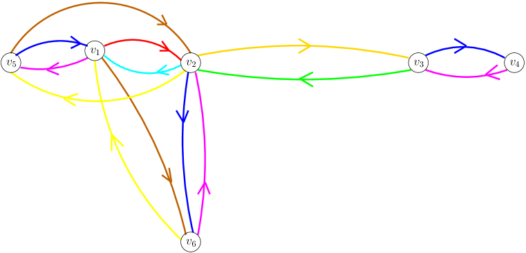
Figure 2.4: Edge coloring of communication graph shown in Figure 2.2 corresponding to the link schedule shown in Figure 2.1(b).

Given the above representations, a point to point link schedule $\Psi(\cdot)$ for an STDMA wireless network $\Phi(\cdot)$ can be considered as equivalent to assigning a unique color to every edge in the communication graph, such that transmitter-receiver pairs with the same color transmit simultaneously in a particular time slot. For the example network considered, the link schedule shown in Figure 2.1(b) corresponds to the coloring of the edges of the communication graph shown in Figure 2.4. Time slots 1, 2, 3, 4, 5, 6, 7 and 8 in $\Psi(\cdot)$ correspond to colors red, blue, green, magenta, yellow, cyan, brown and gold in $\mathcal{E}_{c}$ respectively. Note that a coloring algorithm that uses the least number of colors also minimizes the schedule length. This aspect is further addressed in subsequent sections.

2.2.2 Review of Algorithms

In this section, we provide an overview of past research in the field of STDMA point to point link scheduling algorithms based on the protocol interference model. The protocol interference model is widely studied in literature because of its simplicity. It has been usually employed to model networks such as Carrier Sense Multiple Access with Collision Avoidance (CSMA/CA) based WLANs [27], [25]. Centralized algorithms [16], [28], [29], [30], [25] as well as distributed algorithms [31] have been proposed for generating link schedules based on the protocol interference model.

A link scheduling algorithm based on the protocol interference model utilizes a communication or two-tier graph model of the STDMA network to determine a point to point link schedule [32], [33]. Algorithms based on the protocol interference model for assigning links to time slots (equivalently, colors) require that two communication edges $v_{i}\stackrel{{\scriptstyle c}}{{\rightarrow}}v_{j}$ and $v_{k}\stackrel{{\scriptstyle c}}{{\rightarrow}}v_{l}$ can be colored the same if and only if:

1. vertices $v_{i}$, $v_{j}$, $v_{k}$, $v_{l}$ are all mutually distinct, i.e., there is no primary edge conflict, and

2. $v_{i}\rightarrow v_{l}\not\in\mathcal{G}(\cdot)$ and $v_{k}\rightarrow v_{j}\not\in\mathcal{G}(\cdot)$, i.e, there is no secondary edge conflict.

The first criterion is based on the operational constraint (2.1). The second criterion states that a node cannot receive a packet if it lies within the interference range of any other transmitting node. A scheduling algorithm utilizes various graph coloring methodologies to obtain a non-conflicting link schedule, i.e., a link schedule devoid of primary and secondary edge conflicts.

To maximize the throughput of an STDMA network, algorithms based on the protocol interference model seek to minimize the total number of colors used to color all the communication edges of $\mathcal{G}(\cdot)$. This will in turn minimize the schedule length. It is well known that for an arbitrary communication graph, the problem of determining a minimum length schedule (optimal schedule) is NP-hard [16], [29]. Hence, the approach followed in the literature is to devise algorithms that produce close to optimal (sub-optimal) solutions. The efficiency of a sub-optimal algorithm is typically measured in terms of its computational (run time) complexity and performance guarantee (approximation factor).

The concept of STDMA for wireless networks was formalized in [28]. The authors assume a multihop packet radio network with fixed node locations and consider the problem of assigning an integral number of slots to every link in an STDMA cycle (frame). To solve this problem, they model the network by a communication graph, determine a set of maximal cliques and then assign a certain number of slots to all the links in each maximal clique. Finally, the authors develop a fluid approximation for the mean system delay and validate it using simulations.

In [29], the authors consider pre-specified link demands in a spread spectrum packet radio network. They formulate the problem as a linear optimization problem and use the ellipsoid algorithm [34] to solve the problem. They assume that the desired link data rates are rational numbers and develop a strongly polynomial algorithm that computes a minimum length schedule. Finally, they consider the problem of link scheduling to satisfy pre-specified end-to-end demands in the network. They formulate this problem as a multicommodity flow problem and describe a polynomial time algorithm that computes a minimum length schedule. As pointed out by the authors, their algorithm is not practical due to its high computational complexity.

A significant work in link scheduling under protocol interference model is reported in [16], in which the authors show that tree networks can be scheduled optimally, oriented graphs can be scheduled near-optimally and arbitrary networks can be scheduled such that the schedule is bounded by a length proportional to the graph thickness times the optimum number of colors.

In [16], the authors seem to have missed a subtle point that colors from previously colored oriented graphs can be used to color the current oriented graph. Instead, they use a fresh set of colors to color each successive oriented graph. Consequently, their algorithm leads to a higher numbers of colors, especially if the number of oriented graphs is large. The authors employ such a heuristic primarily to upper bound the number of colors used by the algorithm ([16], Lemma 3.4) and consequently obtain bounds on the running time complexity and performance guarantee of the algorithm ([16], Theorem 3.3). Though the ArboricalLinkSchedule algorithm has nice theoretical properties such as low computational complexity, it can be shown that it may yield a higher number of colors in practice. This leads to lower network throughput.

We should point out here that, if we modify the ArboricalLinkSchedule algorithm to reuse colors from previously colored oriented graphs to color the current oriented graph, then the schedule length will always be lower than the schedule length obtained by the ArboricalLinkSchedule algorithm. This can lead to higher network throughput. We develop this idea further in Chapter 3. Furthermore, we show that this can be achieved with only a slight increase in computational complexity.

In [26], the authors investigate throughput bounds for a given wireless network and traffic workload under the protocol interference model. They use a conflict graph to represent interference constraints. The problem of finding maximum throughput for a given source-destination pair under the flexibility of multipath routing is formulated as a linear program with flow constraints and conflict graph constraints. They show that this problem is NP-hard and describe techniques to compute lower and upper bounds on throughput. Finally, the authors numerically evaluate throughput bounds and computation time of their heuristics for simple network scenarios and IEEE 802.11 MAC (bidirectional MAC). Though the authors provide a general framework for joint routing and scheduling, they neither derive the computational complexity of their heuristics nor describe their link scheduling algorithm explicitly.

Recently, in [25], the authors investigate joint link scheduling and routing under the protocol interference model for a wireless mesh network consisting of static mesh routers and mobile client devices. Assuming that $l(u)$ denotes the aggregate traffic demand on node $u$, they consider the problem of maximizing $\lambda$, such that at least $\lambda l(u)$ amount of traffic can be routed from each node $u$ to a fixed gateway node. Since this problem is NP-hard, the authors propose heuristics based on linear programming and re-routing flows on the communication graph. They derive the worst case bound of their algorithm and evaluate its performance via simulations. Though the authors make a reasonable attempt to solve the joint routing and scheduling problem, their algorithm is extremely complex and brute force in nature. Furthermore, the authors have not provided intuitive arguments for their algorithm.

Another recent work which jointly investigates link scheduling and routing under protocol interference model is reported in [30]. The authors consider wireless mesh networks with half duplex and full duplex orthogonal channels, wherein each node can transmit to at most one node and/or receive from at most $k$ nodes ($k\geqslant 1$) during any time slot. They investigate the joint problem of routing and scheduling to analyze the achievability of a given rate vector between multiple source-destination pairs. The scheduling algorithm is equivalent to an edge-coloring on a multi-graph representation and the corresponding necessary conditions lead the routing problem to be formulated as a linear optimization problem. The authors describe a polynomial time approximation algorithm to obtain an $\epsilon$-optimal solution of the routing problem using the primal dual approach. Finally, they evaluate the performance of their algorithms via simulations.

It has been observed that high data rates are achievable in a wireless mesh network by allowing a node to transmit to only one neighboring node at fixed peak power in any time slot [30]. We point out here that a similar assumption of uniform transmission power has been made in our system model in subsequent chapters of the thesis.

Algorithms based on the protocol interference model represent the network by a communication or two-tier graph and employ a plethora of techniques from graph theory [35] and approximation algorithms [36], [37] to devise heuristics which yield a minimum length schedule. Consequently, such algorithms have the advantage of low computational complexity (in general). However, recent research suggests that these algorithms result in low network throughput. This aspect is further illustrated in the following section.

2.3 Limitations of Algorithms based on Protocol Interference Model

Due to its inherent simplicity, the protocol interference model has been traditionally employed to represent a wide variety of wireless networks. However, it leads to low network throughput in wireless mesh networks. To emphasize this point, we provide examples to demonstrate that algorithms based on the protocol interference model can result in schedules that yield low network throughput.

Intuitively, the protocol interference model divides the deployment region of the STDMA wireless network into “communication zones” and “interference zones”. This transforms the scheduling problem to an edge coloring problem for the communication graph representation of the network. However, this simplification can result in schedules that do not satisfy the SINR threshold condition (2.7).

Specifically, algorithms based on the protocol interference model do not necessarily maximize the throughput of an STDMA wireless network because:

1. They can lead to high cumulative interference at a receiver, due to hard-thresholding based on communication and interference radii [32], [33]. This is because the SINR at receiver $r_{i,j}$ decreases with an increase in the number of concurrent transmissions $M_{i}$, while the communication radius $R_{c}$ and the interference radius $R_{i}$ have been defined for a single transmission only.

   

   Figure 2.5: An STDMA wireless network with six nodes.

   

   Figure 2.6: Two-tier graph model of the STDMA wireless network described by Figure 2.5 and Table 2.1.

   

   Figure 2.7: Subgraph of two-tier graph shown in Figure 2.6.

   

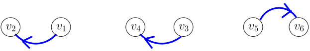
   Figure 2.8: Coloring of subgraph shown in Figure 2.7.

   

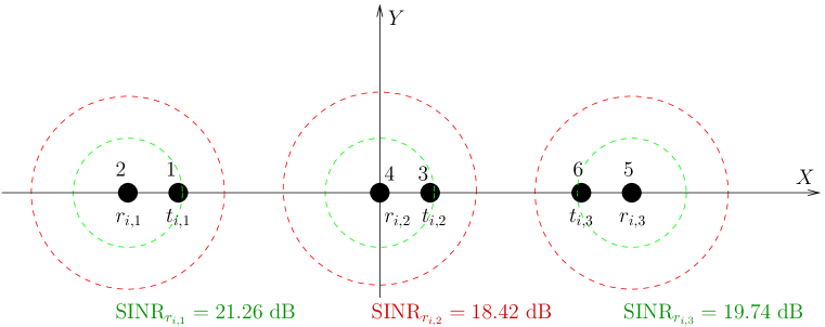
   Figure 2.9: Point to point link scheduling algorithms based on protocol interference model can lead to high interference.

   For example, consider the STDMA wireless network whose deployment is shown in Figure 2.5. The network consists of six labeled nodes whose coordinates (in meters) are $1\equiv(-360,0)$, $2\equiv(-450,0)$, $3\equiv(90,0)$, $4\equiv(0,0)$, $5\equiv(360,0)$ and $6\equiv(450,0)$. The system parameters are shown in Table 2.1, which yield $R_{c}=100$ m and $R_{i}=177.8$ m. The two-tier graph model of the STDMA network is shown in Figure 2.6; note that interference edges are absent. Consider the transmission requests $1\rightarrow 2$, $3\rightarrow 4$ and $5\rightarrow 6$, which correspond to communication edges of the subgraph shown in Figure 2.7. The communication edges $v_{1}\stackrel{{\scriptstyle c}}{{\rightarrow}}v_{2}$, $v_{3}\stackrel{{\scriptstyle c}}{{\rightarrow}}v_{4}$ and $v_{5}\stackrel{{\scriptstyle c}}{{\rightarrow}}v_{6}$ shown in Figure 2.7 do not have primary or secondary edge conflicts. To minimize the number of colors, such an algorithm will color these edges with the same color, as shown in Figure 2.8. Equivalently, transmissions $1\rightarrow 2$, $3\rightarrow 4$ and $5\rightarrow 6$ will be scheduled in the same time slot, say time slot $i$. However, our computations show that the SINRs at receivers $r_{i,1}$, $r_{i,2}$ and $r_{i,3}$ are $21.26$ dB, $18.42$ dB and $19.74$ dB respectively. Figure 2.9 shows the nodes of the network along with the labeled transmitter-receiver pairs, receiver-centric communication and interference zones and the SINRs at the receivers. From the SINR threshold condition (2.6), transmission $t_{i,1}\rightarrow r_{i,1}$ is successful, while transmissions $t_{i,2}\rightarrow r_{i,2}$ and $t_{i,3}\rightarrow r_{i,3}$ are unsuccessful. This leads to low network throughput.

2. Moreover, these algorithms can be extremely conservative and result in higher number of colors.

   

   Figure 2.10: An STDMA wireless network with four nodes.

   

   Figure 2.11: Two-tier graph model of STDMA wireless network described by Figure 2.10 and Table 2.1.

   

   Figure 2.12: Subgraph of two-tier graph shown in Figure 2.11.

   

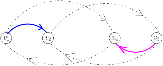
   Figure 2.13: Coloring of subgraph shown in Figure 2.12.

   

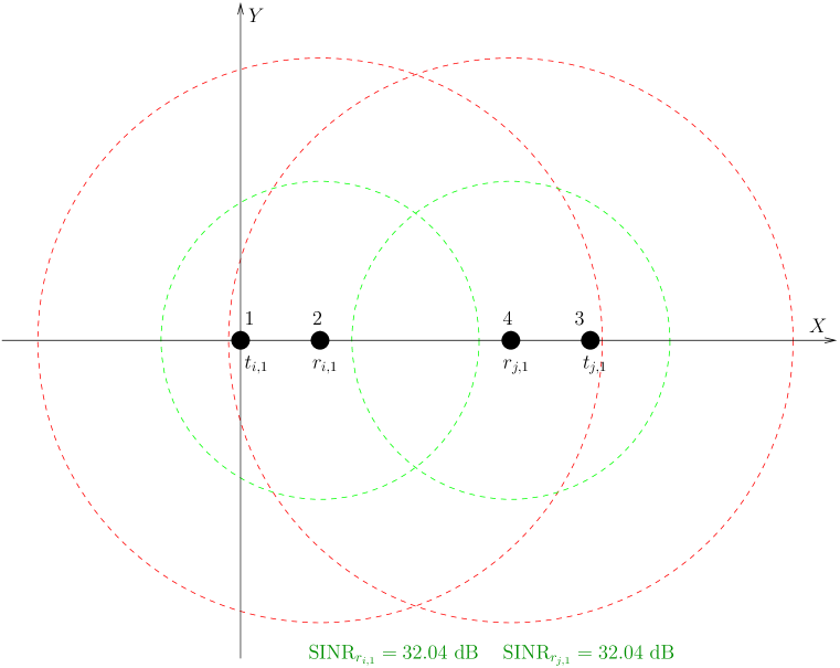
   Figure 2.14: Point to point link scheduling algorithms based on protocol interference model can lead to higher number of colors.

   

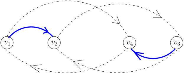
   Figure 2.15: Alternative coloring of subgraph shown in Figure 2.12.

   

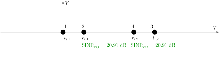
   Figure 2.16: A point to point link schedule corresponding to Figure 2.15 that yields lower number of colors.

   For example, consider the STDMA wireless network whose deployment is shown in Figure 2.10. The network consists of four labeled nodes whose coordinates (in meters) are $1\equiv(0,0)$, $2\equiv(50,0)$, $3\equiv(220,0)$ and $4\equiv(170,0)$. The system parameters are shown in Table 2.1, which lead to $R_{c}=100$ m and $R_{i}=177.8$ m. The two-tier graph model of the STDMA network is shown in Figure 2.11. Consider the transmission requests $1\rightarrow 2$ and $3\rightarrow 4$, which correspond to communication edges of the subgraph shown in Figure 2.12. The communication edges $v_{1}\stackrel{{\scriptstyle c}}{{\rightarrow}}v_{2}$ and $v_{3}\stackrel{{\scriptstyle c}}{{\rightarrow}}v_{4}$ shown in Figure 2.12 have secondary edge conflicts. Hence, such an algorithm will typically color these edges with different colors, as shown in Figure 2.13. Equivalently, a link scheduling algorithm based on the protocol interference model will schedule transmissions $1\rightarrow 2$ and $3\rightarrow 4$ in different time slots, say time slots $i$ and $j$ respectively, where $i\neq j$. Our computations show that the resulting SINRs at receivers $r_{i,1}$ and $r_{j,1}$ are both equal to $32.04$ dB. Figure 2.14 shows the nodes of the network along with the labeled transmitter-receiver pairs, receiver-centric communication and interference zones and SINRs at the receivers. Observe that, with an algorithm based on the protocol interference model, the SINRs at both receivers are well above the communication threshold of $20$ dB. Alternatively, consider an algorithm (perhaps based on the physical interference model) that schedules transmissions $1\rightarrow 2$ and $3\rightarrow 4$ in the same time slot, say time slot $i$. The corresponding edge coloring is shown in Figure 2.15. Our computations show that the resulting SINRs at receivers $r_{i,1}$ and $r_{j,1}$ are both equal to $20.91$ dB, which are also above the communication threshold. Figure 2.16 shows the nodes of the network along with the labeled transmitter-receiver pairs and SINRs at the receivers. In essence, with the alternate algorithm, both transmissions $t_{i,1}\rightarrow r_{i,1}$ and $t_{i,2}\rightarrow r_{i,2}$ are successful, since signals levels are so high at the receivers that strong interferences can be tolerated. In summary, a point to point link scheduling algorithm based on the protocol interference model will typically schedule the above transmissions in different slots and yield lower network throughput compared to the alternate algorithm.

3. Lastly, these algorithms are not aware of the topology of the network, i.e., they determine a link schedule without being cognizant of the exact positions of the transmitters and receivers.

The above examples demonstrate that scheduling algorithms based on the protocol interference model can result in low network throughput. Observe that algorithms that construct an approximate model of the STDMA network (two tier graph or communication graph) and focus on minimizing the schedule length do not necessarily maximize network throughput. This observation is developed into a proposal for an appropriate performance metric in Section 2.6.

Since link scheduling algorithms based on the protocol interference model yield low throughput, researchers have propounded algorithms based on the physical interference model to improve the throughput of STDMA wireless networks. To achieve higher throughput, one possible technique is to model the STDMA network by a communication graph and check SINR threshold conditions during assignment of links to time slots; this is the approach most commonly employed, for example in [27], [32], [38]. The other technique is to incorporate SINR threshold conditions into a special graph model of the network; this approach is more challenging and (to the best of our knowledge) is considered only in research work such as [39], [40], [41]. Research papers which employ the former approach are reviewed in Section 2.4, while research papers which employ the latter approach are reviewed in Section 2.5.

2.4 Link Scheduling based on Communication Graph Model and SINR Conditions

In this section, we examine recent research in link scheduling based on modeling the STDMA network by a communication graph and verifying SINR conditions at the receivers. Though algorithms based on this model [24], [42], yield higher throughput, they usually result in higher computational complexity than algorithms based on the protocol interference model.

In [27], the authors investigate throughput improvement in an IEEE 802.11 like wireless mesh network with CSMA/CA channel access scheme replaced by STDMA. For a successful packet transmission, they mandate that two-way communication be successful, i.e., a packet transmission is defined to be successful if and only if both data and acknowledgement packets are received successfully. Under this “extended physical interference model”, they present a greedy algorithm which computes a point to point link transmission schedule in a centralized manner. Assuming uniform random node distribution and using results from occupancy theory [43], they derive an approximation factor for the length of this schedule relative to the shortest schedule. Though the analysis presented in [27] is novel, their model is restrictive because it is only applicable to wireless networks using link-layer reliability protocols.

The throughput performance of link scheduling algorithms based on two-tier graph model $\mathcal{G}(\mathcal{V},\mathcal{E}_{c}\,\cup\,\mathcal{E}_{i})$ has been analyzed under physical interference conditions in [32]. The authors determine the optimal number of simultaneous transmissions by maximizing a lower bound on the throughput and subsequently propose Truncated Graph-Based Scheduling Algorithm (TGSA), an algorithm that provides probabilistic guarantees for network throughput. Though the analysis presented in [32] is mathematically elegant and based on the Edmundson-Madansky bound [44], [45], their algorithm does not yield high network throughput. This is because the partitioning of a maximal independent set of communication edges into multiple subsets (time slots) is arbitrary and not based on network topology, which can lead to significant interference in certain regions of the network. This is further elucidated by the simulation results in Chapter 3.

The performance of algorithms based on the protocol interference model versus those based on communication graph model and SINR conditions is evaluated and compared in [33]. To generate a non-conflicting link schedule based on the protocol interference model, the authors use a two-tier graph model with certain SINR threshold values chosen based on heuristics and examples. To generate a conflict-free point to point link schedule based on the physical interference model, the authors employ a method suggested in [46] which describes heuristics based on two path loss models, namely terrain-data based ground wave propagation model and Vogler’s five knife-edge model. Their simulations results indicate that, under a Poisson arrival process, algorithms based on the protocol interference model result in higher average packet delay than algorithms based on communication graph model and SINR conditions.

In [42], the authors investigate the tradeoff between the average number of concurrent transmissions (spatial reuse) and sustained data rate per node for an IEEE 802.11 wireless network. They show that spatial reuse depends only on the ratio of transmit power to carrier sense threshold [6]. Keeping the carrier sense threshold fixed, they propose a distributed power and rate control algorithm based on interference measurement and evaluate its performance via simulations.

In [24], the authors investigate mitigation of inter-flow interference in an IEEE 802.11e wireless mesh network from a temporal-spatial diversity perspective. Measurements of received signal strengths are used to construct a virtual coordinate system to identify concurrent transmissions with minimum inter-flow interference. Based on this new coordinate system, one of the nodes, designated as gateway node, determines the scheduling order for downlink frames of different connections. Through extensive simulations with real-life measurement traces, the authors demonstrate throughput improvement with their algorithm.

Algorithms based on representing the network by a communication graph and verifying SINR threshold conditions yield higher network throughput than algorithms based on the protocol interference model. However, this is achieved at the cost of higher computational complexity. Furthermore, the gains in throughput may not be significant enough to justify the increase in computational complexity. This has prompted few researchers to solve the link scheduling problem in a more fundamental manner. These researchers have proposed an altogether different model of the network, termed as SINR graph model, and developed heuristics. Such algorithms are reviewed in the following section.

2.5 Link Scheduling based on SINR Graph Model

In literature, many authors refer to algorithms based on communication graph model and checking SINR conditions as “algorithms based on physical interference model”. In this thesis, only algorithms that embed SINR threshold conditions into an appropriate graph model of the network are referred to as “algorithms based on the physical interference model”. Though the physical interference model is more realistic, algorithms based on this model [39], [40], [41] have, in general, higher computational complexity than algorithms based on the protocol interference model.

Point to point link scheduling for power-controlled STDMA networks under the physical interference model is analyzed in [39]. The authors define scheduling complexity as the minimum number of time slots required for strong connectivity of the graph constructed from the point to point link schedule. They develop an algorithm employing non-linear power assignment and show that its scheduling complexity is polylogarithmic in the number of nodes. In a related work [40], the authors investigate the time complexity of scheduling a set of communication requests in an arbitrary network. They consider a “generalized physical model” wherein the actual received power of a signal can deviate from the theoretically received power by a multiplicative factor. Their algorithm successfully schedules all links in time proportional to the squared logarithm of the number of nodes times the static interference measure [47]. Though the authors of [39], [40] allow non-uniform transmission power at all nodes and develop novel algorithms, their algorithms are impractical. This is because wireless devices have constraints on maximum transmission power, while the algorithms in [39], [40] can result in arbitrarily high transmission power at some nodes.

In [26], the authors provide a general framework for computation of throughput bounds for a given wireless network and traffic workload. Though their work primarily focuses on the protocol interference model, they briefly allude to the physical interference model too. Specifically, they describe a technique to construct a weighted conflict graph to represent interference constraints. They briefly describe methods to compute lower and upper bounds on throughput and the issues involved therein. However, the authors do not describe simulation results under the physical interference model, perhaps due to the tremendous complexity incurred in solving linear programs for representative network scenarios.

Remark 2.5.1.

Under physical interference model, the weighted conflict graph $F(V_{F},E_{F})$ [26] is constructed from the network as follows. Let $S_{ij}:=\frac{P}{D^{\beta}(i,j)}$ denote the received signal power at node $j$ due to the transmission from node $i$. In $F(\cdot)$, a vertex corresponds to a directed link $l_{ij}$ (equivalently, node pair $(i,j)$) provided $\frac{S_{ij}}{N_{0}}\geqslant\gamma_{c}$. $F(\cdot)$ is a perfect graph wherein the weight $w_{ij}^{pq}$ of the directed edge from vertex $l_{pq}$ to vertex $l_{ij}$ is given by $w_{ij}^{pq}=\frac{S_{pj}}{\frac{S_{ij}}{\gamma_{c}}-N_{0}}$.

We should point out here that, analogous to a conflict graph, an SINR graph representation of an STDMA wireless network has been proposed by us in Chapter 4. Furthermore, the authors of [26] do not propose any specific link scheduling algorithm and use the weighted conflict graph only to compute bounds on network throughput. On the other hand, we use an SINR graph representation of the network under the physical interference model and develop a link scheduling algorithm with lower time complexity and demonstrably superior performance.

More specifically, in Chapter 4, we investigate link scheduling for STDMA wireless networks under the physical interference model. Unlike [39], [40], we assume that a node transmits at fixed power, i.e., we assume uniform power assignment. Moreover, unlike [39], [40], we do not assume a minimum distance of unity between any two nodes. Consequently, our system model is more practical than those of [39], [40]. Under these realistic assumptions, we propose a link scheduling algorithm based on an SINR graph representation of the network. In the SINR graph, weights of the edges correspond to interferences between pairs of nodes. We prove the correctness of the algorithm and derive its computational complexity. We demonstrate that the proposed algorithm achieves higher throughput than existing algorithms, without any increase in computational complexity.

So far, we have provided a brief glimpse into three classes of link scheduling algorithms, each with its relative merits and demerits. For example, algorithms based on the protocol interference model have low computational complexity and are simple to implement, but yield low network throughput. On the other hand, algorithms based on SINR graph representation have higher computational complexity and are more cumbersome to implement, but achieve higher network throughput. Also, there exist algorithms based on communication graph and SINR conditions whose performance characteristics lie between these two classes. Hence, in general, these three classes of algorithms exhibit a tradeoff between complexity and performance. Finally, algorithms based on the protocol interference model are better suited to model WLANs, while the latter two classes of algorithms are better suited to model wireless mesh networks. For these reasons, we investigate and develop algorithms from each of these classes in this thesis.

Prior to proposing efficient algorithms in each of these classes, we seek to address the following question: Is schedule length an appropriate performance metric for an algorithm that considers the SINR threshold condition (2.6) as the criterion for successful packet reception? In other words, should algorithms based on communication graph and SINR conditions and algorithms based on SINR graph representation focus on minimizing the schedule length? We answer this important question in detail in the following section.

2.6 Spatial Reuse as Performance Metric

In literature, link scheduling algorithms have only focused on minimizing the schedule length. However, algorithms that minimize the schedule length do not necessarily maximize network throughput, as explained in Section 2.3. Thus, from a perspective of maximizing network throughput observed by the physical layer, it is imperative to consider a performance metric that takes into account SINR threshold condition (2.6) as the criterion for successful packet reception, i.e., a metric also suitable for the physical interference model. We propose such a performance metric, spatial reuse, in this section. We show that maximizing spatial reuse directly translates to maximizing network throughput.

Consider an STDMA wireless network that operates over $(k_{2}-k_{1}+1)$ time slots $k_{1},k_{1}+1,\ldots,k_{2}-1,k_{2}$. The total number of successfully scheduled links from slot $k_{1}$ to slot $k_{2}$ is

$$\tau[k_{1},k_{2}] = \sum_{i=k_{1}}^{k_{2}}\sum_{j=1}^{M_{i}}I(\mbox{SINR}_{r_{ij}}\geqslant\gamma_{c}).$$ (2.11)

So, the number of successfully scheduled links per time slot from slot $k_{1}$ to slot $k_{2}$ is

$$\eta[k_{1},k_{2}] = \frac{\sum_{i=k_{1}}^{k_{2}}\sum_{j=1}^{M_{i}}I(\mbox{SINR}_{r_{ij}}\geqslant\gamma_{c})}{k_{2}-k_{1}+1}.$$ (2.12)

We define spatial reuse $\sigma$ as the limiting value of $\eta[k_{1},k_{2}]$ (assuming that the limit exists). In other words, spatial reuse is the limiting value of $\eta[k_{1},k_{2}]$ as the duration of the time interval becomes very large. Mathematically,

Spatial Reuse $$:= \lim_{|k_{2}-k_{1}|\rightarrow\infty}\eta[k_{1},k_{2}],$$

$$\therefore\sigma = \lim_{|k_{2}-k_{1}|\rightarrow\infty}\frac{\sum_{i=k_{1}}^{k_{2}}\sum_{j=1}^{M_{i}}I(\mbox{SINR}_{r_{ij}}\geqslant\gamma_{c})}{k_{2}-k_{1}+1}.$$ (2.13)

Assuming a constant data rate of $R$ bits per second on each successful link and a slot duration of $\tau_{s}$ seconds, the (aggregate) network throughput is given by $\sigma R\tau_{s}$ bits per second. Thus, spatial reuse is directly proportional to network throughput. Note that spatial reuse is cognizant of the physical interference model, thereby making it an appropriate performance metric for the comparison of various link scheduling algorithms.

The fact that the interference at a receiver is an increasing function of the number of concurrent transmissions in a time slot limits the value of spatial reuse (for a given STDMA network). More specifically, if too many transmissions are scheduled in a single time slot, the interference at some receivers will be high enough to drive the SINRs below the communication threshold, leading to lower spatial reuse. Therefore, for a given STDMA network, there are certain fundamental limits (upper bounds) on the spatial reuse.

In our system model, we only consider static link schedules, i.e., the same fixed pattern of slots repeats cyclically. Hence, for our system model, the equation for spatial reuse, (2.13), can be simplified to

Spatial Reuse $$= \sigma\;=\;\frac{\sum_{i=1}^{C}\sum_{j=1}^{M_{i}}I(\mbox{SINR}_{r_{ij}}\geqslant\gamma_{c})}{C}.$$ (2.14)

The essence of STDMA is to have a reasonably large number of concurrent and successful transmissions. For a network which is operational for a long period of time, say $L$ time slots, the total number of successfully received packets is $L\sigma$. Thus, a high value of spatial reuse directly translates to higher network throughput and the number of colors $C$ is relatively unimportant. Hence, spatial reuse

turns out to be a crucial metric for the comparison of different STDMA algorithms in Chapters 3, 4 and 5.

Chapter 3 Point to Point Link Scheduling based on Communication Graph Model

We begin our investigation in link scheduling by critically examining the ArboricalLinkSchedule algorithm proposed in [16]. The algorithm is based only on the communication graph (protocol interference model) and seeks to minimize the schedule length. Though ArboricalLinkSchedule has good properties such as low computational complexity, it can yield higher schedule length in practice. Towards this end, we propose a novel modification to ArboricalLinkSchedule that results in lower schedule length. We compare the performance of the modified algorithm with the ArboricalLinkSchedule algorithm and derive its run time (computational) complexity in Section 3.1. We then propose the ConflictFreeLinkSchedule point to point link scheduling algorithm, which is based on communication graph model and SINR conditions, in Section 3.2. The performance of the proposed algorithm is compared with existing link scheduling algorithms under various wireless channel conditions. We show that the proposed algorithm has polynomial run time complexity. Finally, we summarize the implications of our work.

3.1 ArboricalLinkSchedule Algorithm Revisited

In this section, we propose a modification to the ArboricalLinkSchedule point to point link scheduling algorithm. Since both the original algorithm and the proposed modification are based on the protocol interference model, we compare their performance in terms of average schedule length. Finally, we also derive the run time complexity of the modified algorithm.

Our system model and notation are same as described in Section 2.2. We seek an algorithm that determines a minimum length point to point link schedule for an STDMA wireless network under the protocol interference model. For consistency with the graph model described in [16], we assume that the STDMA wireless network $\Phi(\cdot)$ is modeled by the communication graph $\mathcal{G}_{c}(\mathcal{V},\mathcal{E}_{c})$ only, i.e., interference edges are absent $(\mathcal{E}=\mathcal{E}_{c})$.

It is well known that, under the protocol interference model, the problem of determining an optimal schedule, i.e., a minimum length schedule, is NP-hard [48]. As pointed out in Section 2.2.1, this is closely related to the problem of coloring all edges of the communication graph with minimum number of colors, which is also known to be NP-hard [16]. Consequently, the only recourse is to devise approximation algorithms (heuristics) and show their efficiency theoretically and experimentally.

One such algorithm, ArboricalLinkSchedule, has been described in [16]. First, the algorithm uses the labeler function to label all the vertices of the communication graph. Next, it partitions the communication graph into edge-disjoint subgraphs, which are termed as “oriented graphs”. Finally, the oriented graphs are colored in sequence. Specifically, the vertices in each oriented graph are scanned in increasing order of label and the unique edge associated with each vertex is colored using the NonConflictingEdge function [16]. The labeler function and the partitioning technique are described later in the section.

In [16], the authors appear to have missed a delicate point that colors from previously colored oriented graphs can be used to color the present oriented graph. Specifically, they use a fresh set of colors to color each successive oriented graph. In our opinion, the authors employ this method to upper bound the number of colors used by the algorithm ([16], Lemma 3.4) and thus derive the running time complexity of the algorithm ([16], Theorem 3.3). However, such a heuristic can potentially lead to a higher number of colors (and higher schedule length) in practice.

Therefore, we propound a modification to the ArboricalLinkSchedule algorithm that reuses colors from previously colored oriented graphs to colors the current oriented graph. The resulting schedule length will always be lower than that of ArboricalLinkSchedule, leading to potentially higher throughput. Our proposed link scheduling algorithm is ALSReuseColors, which considers the communication graph $\mathcal{G}_{c}({\mathcal{V}},\mathcal{E})$ and is described in Algorithm 1.

In Phase 1, we label all the vertices using the labeler function [16]. The labeler function is reproduced in Algorithm 2 for convenience. It is a recursive function that assigns a unique label (from $1$ to $N$) to every vertex of the communication graph. Let $L(w)$ denote the label assigned to vertex $w$. The notation $\mathcal{G}_{r}\setminus\{u\}$ denotes the graph that results when vertex $u$ and all its incident edges are removed from graph $\mathcal{G}_{r}(\cdot)$. At every step in the recursion, it chooses the minimum degree vertex $u$ in the residual graph $\mathcal{G}_{r}(\cdot)$ and assigns it the highest label that has not been assigned so far. Note that vertices with lower degree tend to be assigned higher labels. The labeler function ensures that, for any given node, the number of neighbors with lower labels is much lower than the number of vertices in $\mathcal{G}_{c}(\cdot)$.

In Phase 2, the communication graph $\mathcal{G}_{c}(\cdot)$ is decomposed into what are called as out-oriented and in-oriented graphs $T_{1},T_{2},\ldots,T_{k}$, similar to the technique employed in [16]. Recall that an in-oriented graph is a directed graph in which every vertex has at most one outgoing edge, while an out-oriented graph is a directed graph in which every vertex has at most one incoming edge. Each $T_{i}$ is a forest and every edge of $\mathcal{G}_{c}(\cdot)$ is in exactly one of the $T_{i}$’s. This decomposition is achieved by partitioning graph $G_{c}(\cdot)$, the undirected equivalent of $\mathcal{G}_{c}(\cdot)$, into undirected forests. The number of forests can be minimized by using techniques from Matroid theory ([49], $k$-forest problem). However, this optimal decomposition requires extensive computation. Hence, we adopt a faster albeit non-optimal approach of using successive breadth first searches [50] to decompose $G_{c}(\cdot)$ into undirected forests. Each undirected forest is further mapped to two directed forests. In one forest, the edges in every connected graph point away from the root and every vertex has at most one incoming edge, thus producing an out-oriented graph. In the other forest, the edges in every connected graph point toward the root and every vertex has at most one outgoing edge, thus producing an in-oriented graph.

In Phase 3, the oriented graphs are considered sequentially. For each oriented graph, the vertices are considered in increasing order of label and the unique edge associated with each vertex is colored using the NCEReuseColors function. The NCEReuseColors function is explained in Algorithm 3. For the edge $x$ under consideration, it discards any color from any oriented graph that has an edge with a primary or secondary conflict with $x$. It returns the least color among the residual set of non-conflicting colors from all oriented graphs colored so far. If no non-conflicting color from any oriented graph is found, it returns a new color.

Algorithm 1 ALSReuseColors

1:  input: Directed communication graph $\mathcal{G}_{c}(\mathcal{V},\mathcal{E})$

2:  output: A coloring $C:\mathcal{E}\rightarrow\{1,2,\ldots\}$

3:  $n\leftarrow\mbox{labeler}(\mathcal{G}_{c})$ {Phase 1}

4:  use successive breadth first searches to partition $\mathcal{G}_{c}(\cdot)$ into oriented graphs $T_{i}$, $1\leqslant i\leqslant k$ {Phase 2}

5:  for $i\leftarrow 1\mbox{ to }k$ do {Phase 3 begins}

6:     for $j\leftarrow 1\mbox{ to }n$ do

7:        if $T_{i}$ is out-oriented then

8:           let $x=(s,d)$ be such that $L(d)=j$

9:        else

10:           let $x=(s,d)$ be such that $L(s)=j$

11:        end if

12:        $C(x)\leftarrow\mbox{NCEReuseColors}(x)$

13:     end for

14:  end for{Phase 3 ends}

Algorithm 2 integer labeler($\mathcal{G}_{r}$)

1:  if $\mathcal{G}_{r}(\cdot)$ is not empty then

2:     let $u$ be a vertex of $\mathcal{G}_{r}(\cdot)$ of minimum degree

3:     $L(u)\leftarrow 1+\mbox{labeler}(\mathcal{G}_{r}\setminus\{u\})$

4:  else

5:     return $0$

6:  end if

Algorithm 3 integer NCEReuseColors($x$)

1:  input: Directed communication graph $\mathcal{G}_{c}(\mathcal{V},\mathcal{E})$

2:  output: A non-conflicting color

3:  ${\mathcal{C}}\leftarrow\mbox{set of existing colors}$

4:  $\mathcal{C}_{1}\leftarrow\{C(h):$ $h$ is colored and $x$ and $h$ have a primary edge conflict$\}$

5:  $\mathcal{C}_{2}\leftarrow\{C(h):$ $h$ is colored and $x$ and $h$ have a secondary edge conflict$\}$

6:  ${\mathcal{C}}_{nc}={\mathcal{C}}\setminus\{\mathcal{C}_{1}\cup\mathcal{C}_{2}\}$

7:  if ${\mathcal{C}}_{nc}\neq\phi$ then

8:     return the least color $\in$ $\mathcal{C}_{nc}$

9:  else

10:     return $|\mathcal{C}|+1$

11:  end if

3.1.1 Performance Results

In the simulation experiment, every node location is generated randomly, using a uniform distribution for its $X$ and $Y$ coordinates in the deployment area. We assume that the deployment region is a square of length $L$. Thus, if $(X_{j},Y_{j})$ are the Cartesian coordinates of $j^{th}$ node, then $X_{j}\sim U[0,L]$ and $Y_{j}\sim U[0,L]$. The values chosen for system parameters $P$, $\gamma_{c}$, $\beta$ and $N_{0}$, are prototypical values of system parameters in wireless networks [42]. After generating random positions for $N$ nodes, we have complete information of $\Phi(\cdot)$. Using (2.4), we compute the communication range, and then map the STDMA network $\Phi(\cdot)$ to the communication graph $\mathcal{G}_{c}(\cdot)$. Once the schedule $\Psi(\cdot)$ is computed by every algorithm, we know its schedule length $|\mathcal{C}|$. For a given set of parameters $(N,L,R_{c})$, we calculate the average schedule length by averaging $|\mathcal{C}|$ over 1000 randomly generated networks. Keeping all other parameters fixed, we observe the effect of increasing the number of nodes on the average schedule length. In our experiments, we compare the performance of the following algorithms:

• ArboricalLinkSchedule [16],

• Proposed ALSReuseColors.

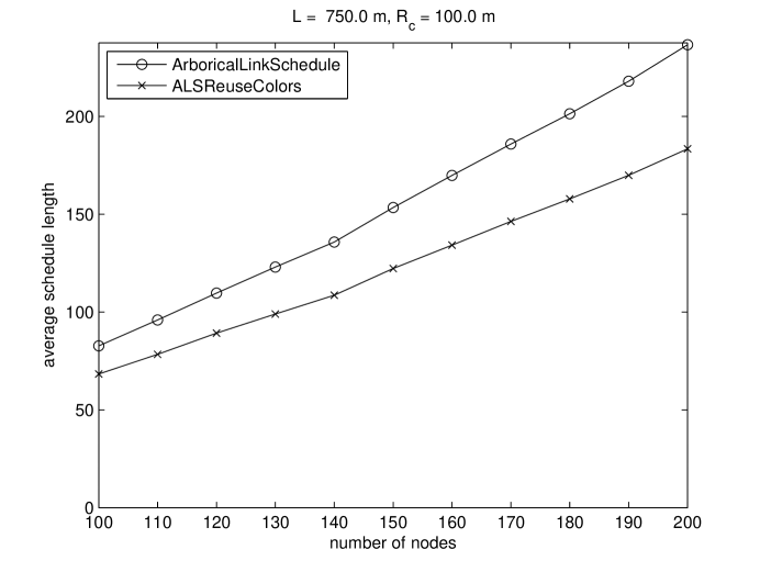
Figure 3.1: Schedule length vs. number of nodes.

We assume that $P=10$ mW, $\beta=4$, $N_{0}=-90$ dBm and $\gamma_{c}=20$ dB. From (2.4), we obtain $R_{c}=100$ m. We assume that $L=750$ m, and vary the number of nodes from 100 to 200 in steps of 10. Figure 3.1 plots the average schedule length vs. number of nodes for both the algorithms.

For both the algorithms, we observe that average schedule length increases almost linearly with the number of nodes. The average schedule length of ALSReuseColors is about $23\%$ lower than that of ArboricalLinkSchedule.

Note that an increase in the number of nodes in a given geographical area leads to an increase in the number of edges incident on a vertex and a subsequent increase in the number of oriented graphs. ArboricalLinkSchedule, which is based on using a fresh set of colors for each oriented graph, requires increasingly higher number of colors to color the communication graph compared to ALSReuseColors. Consequently, the gap between the average schedule lengths increases with number of nodes in Figure 3.1.

3.1.2 Analytical Results

We now derive upper bounds on the running time (computational) complexity of the ALSReuseColors algorithm. With respect to the communication graph ${\mathcal{G}}_{c}({\mathcal{V}},\mathcal{E})$, let:

$$e = \mbox{number of edges},$$

$$v = \mbox{number of vertices},$$

$$\rho = \mbox{maximum degree of any vertex},$$

$$\theta =$$ thickness of the graph

$$:= {\mathcal{G}}_{c}(\cdot)$$ minimum number of planar graphs into which the undirected equivalent of

$$\mbox{can be partitioned},$$

$$\omega = \mbox{maximum number of neighbors with lower labels (for any vertex)}.$$

Recall that the modified algorithm partitions the communication graph $\mathcal{G}_{c}(\cdot)$ into oriented graphs $T_{1},T_{2},\ldots,T_{k}$, and colors the oriented graphs in that order. $T_{1}$ is termed as the first oriented graph, while any oriented graph $T_{j}$, where $2\leqslant j\leqslant k$, is termed as a subsequent oriented graph.

Lemma 3.1.1.

Suppose that each vertex of the first oriented graph $T_{1}$ has at most $\omega$ neighbors with lower labels. Then, $T_{1}$ may be colored using no more than $O(\omega\rho)$ colors.

Proof.

This is similar to the proof of Lemma 3.1 in [16]. ∎

Lemma 3.1.2.

Any subsequent oriented graph $T_{j}$, where $2\leqslant j\leqslant k$, can be colored using no more than $O(\rho^{2})$ colors.

Proof.

Figure 3.2: Potential conflicting edges when coloring edge $(u,v)$.

We prove the lemma for an out-oriented graph. A similar proof holds for an in-oriented graph. Let $\mathcal{G}_{c}$ be partitioned into edge-disjoint oriented graphs $T_{1},\ldots,T_{k}$. Consider the coloring of edge $(u,v)$ in $j^{th}$ oriented graph $T_{j}$, where $2\leqslant j\leqslant k$, as shown in Figure 3.2. Now, edges of previously colored oriented graphs $T_{1},\ldots,T_{j-1}$ must also be considered for potential edge conflicts with edge $(u,v)$ of $T_{j}$. Define

$$S_{1} := \Big{\{}(v,x):(v,x)\in\bigcup_{i=1}^{j}T_{i}\mbox{ and $(v,x)$ is colored}\Big{\}},$$

$$S_{2} := \Big{\{}(u,x):(u,x)\in\bigcup_{i=1}^{j}T_{i}\mbox{ and $(u,x)$ is colored}\Big{\}},$$

$$S_{3} := \Big{\{}(y,x_{i}):(y,x_{i})\in\bigcup_{i=1}^{j}T_{i}\mbox{ and $(y,x_{i})$ is colored and }(u,x_{i})\in\mathcal{G}_{c}\Big{\}},$$

$$S_{4} := \Big{\{}(x_{i},y):(x_{i},y)\in\bigcup_{i=1}^{j}T_{i}\mbox{ and $(x_{i},y)$ is colored}\mbox{ and }(x_{i},v)\in\mathcal{G}_{c}\Big{\}}.$$

Any edge which can cause a primary edge conflict with $(u,v)$ must belong to $S_{1}$ or $S_{2}$. Also, any edge which can cause a secondary edge conflict with $(u,v)$ must belong to $S_{3}$ or $S_{4}$. Let $n_{i}=|S_{i}|$ for $i=1,2,3,4$. The lemma reduces to proving that $n_{1}+n_{2}+n_{3}+n_{4}$ is $O(\rho^{2})$.

By definition of maximum vertex degree, $n_{1}\leqslant\rho-1$ and $n_{2}\leqslant\rho-1$. Thus, $n_{1}+n_{2}$ is $O(\rho)$. For the computation of $n_{3}$, we must also consider secondary edge conflicts with edges of previously colored oriented graphs, as shown in Figure 3.2. The worst-case value of $n_{3}$ is $(\rho-1)(\rho-1)$. Thus, $n_{3}$ is $O(\rho^{2})$. Similarly, by considering secondary edge conflicts with edges of previously colored oriented graphs, it follows that $n_{4}$ is $O(\rho^{2})$. Finally, $n_{1}+n_{2}+n_{3}+n_{4}$ is $O(\rho^{2})$. ∎

Lemma 3.1.3.

For the first oriented graph $T_{1}$, the running time of Phase 3 of ALSReuseColors is $O(v\omega\rho)$.

Proof.

This is similar to the proof of Lemma 3.2 in [16]. ∎

Lemma 3.1.4.

For any subsequent oriented graph $T_{j}$, where $2\leqslant j\leqslant k$, the running time of Phase 3 of ALSReuseColors is $O(v\rho^{2})$.

Proof.

From Lemma 3.1.2, for any subsequent oriented graph $T_{j}$, the size of the set of conflicting colors $(\mathcal{C}_{1}\cup\mathcal{C}_{2})$ of function NCEReuseColors is $O(\rho^{2})$. Thus, determining a new color for an edge in Phase 3 of ALSReuseColors takes $O(\rho^{2})$ steps. Since this is done for every label and hence for every vertex, it follows that the overall running time of Phase 3 of ALSReuseColors is $O(v\rho^{2})$. ∎

Theorem 3.1.5.

For an arbitrary graph of thickness $\theta$ and maximum degree $\rho$, ALSReuseColors has a running time of $O(ev\log v+v\theta\rho^{2})$.

Proof.

The running time of the labeler function is $O(e+v\log v)$ using a Fibonacci Heap [51]. The partitioning method of [49] results in a decomposition of a graph of thickness $\theta$ into at most $6\theta$ oriented graphs in time $O(ev\log v)$. Thus, $k\leqslant 6\theta$. From Lemma 3.2 in [16], the first oriented graph $T_{1}$ can be colored in time $O(v\omega\rho)$. However, consider the coloring of $j^{th}$ oriented graph $T_{j}$, where $2\leqslant j\leqslant k$. From Lemma 3.1.4, $T_{j}$ can be colored in time $O(v\rho^{2})$. Hence, the for loop of ALSReuseColors runs in time $O(v\theta\rho^{2})$. Therefore, the overall running time of ALSReuseColors is $O(e+v\log v+ev\log v+v\theta\rho^{2})$. Since $e+v\log v<ev\log v$ holds for any directed graph $\mathcal{G}_{c}(\cdot)$ that models a wireless mesh network, the overall running time of ALSReuseColors simplifies to $O(ev\log v+v\theta\rho^{2})$. ∎

3.1.3 Discussion

In this section, we have considered an STDMA wireless network with uniform transmission power at all nodes and presented an algorithm for point to point link scheduling under the protocol interference model. The proposed algorithm, which is a modification of the ArboricalLinkSchedule algorithm in [16], models the network by a communication graph, partitions the communication graph into edge-disjoint oriented graphs and colors each oriented graph successively. However, unlike [16], we reuse colors from previously colored oriented graphs to color the current oriented graph. The proposed algorithm results in around $26\%$ lower schedule length than that of [16], albeit at the cost of slightly higher computational complexity. Since schedules are constructed only once offline and then used by the network for a long period of time, our approach has the potential of providing higher long-term network throughput.

For the rest of this chapter, we consider point to point link scheduling under the physical interference model. The algorithm developed in this section will be further refined to design a link scheduling algorithm in the next section.

3.2 A High Spatial Reuse Link Scheduling Algorithm

In this section, we propose a point to point link scheduling algorithm based on the communication graph model of an STDMA wireless network as well as SINR computations. We adopt spatial reuse as the performance metric, which has been motivated in Section 2.6. We compare the performance of the proposed algorithm with link scheduling algorithms which utilize a communication graph model of the network. We show that the proposed algorithm achieves higher spatial reuse compared to existing algorithms, without any increase in computational complexity.

3.2.1 Problem Formulation

Our system model and notation are exactly as described in Section 2.2. A link schedule is feasible if it satisfies the following conditions:

1. Operational constraint (2.1).

2. Range constraint: Every receiver is within the communication range of its intended transmitter, i.e.,

   $$D(t_{i,j},r_{i,j})\leqslant R_{c}\;\;\forall\;\;i=1,\ldots,C\;\;\forall\;\;j=1,\ldots,M_{i}.$$ (3.1)

A link schedule $\Psi(\cdot)$ is exhaustive if every pair of nodes which are within communication range occur exactly twice in the link schedule, once with one node being the transmitter and the other node being the receiver, and during another time slot with the transmitter-receiver roles interchanged. Mathematically,

$$D(j,k)\leqslant R_{c}\Rightarrow j\rightarrow k\in\bigcup_{i=1}^{C}{\mathcal{S}}_{i}\;\;\mbox{and}\;\;k\rightarrow j\in\bigcup_{i=1}^{C}{\mathcal{S}}_{i}\;\;\forall\;\;1\leqslant j<k\leqslant N.$$ (3.2)

Our aim is to design a low complexity conflict-free STDMA point to point link scheduling algorithm that achieves high spatial reuse, where spatial reuse is given by (2.14). We only consider STDMA link schedules which are feasible and exhaustive. Thus, our schedules satisfy (2.1), (2.7), (3.1) and (3.2).

3.2.2 Motivation

We briefly describe the essential features of STDMA link scheduling algorithms. An STDMA link scheduling algorithm is equivalent to assigning a unique color to every edge in the communication graph, such that transmitter-receiver pairs corresponding to communication edges with the same color are simultaneously active in a particular time slot, as described in Section 2.2.1. The core of a typical link scheduling algorithm consists of the following functions:

1. An order in which communication edges are considered for coloring.

2. A function which determines the set of all existing colors which can be assigned to the edge under consideration without violating the problem constraints.

3. A BestColor rule to determine which color to assign to the edge under consideration.

The second function considers only operational and range constraints in link scheduling algorithms based on the protocol interference model (equivalently, based on the communication graph). However, in the link scheduling algorithm that we propose, SINR constraints are also taken into account.

Algorithms based on the protocol interference model are inadequate to design efficient link schedules. This is because the communication graph ${\mathcal{G}}_{c}({\mathcal{V}},{\mathcal{E}}_{c})$ is a crude approximation of $\Phi(\cdot)$. Even the two-tier graph ${\mathcal{G}}({\mathcal{V}},{\mathcal{E}}_{c}\,\cup\,{\mathcal{E}}_{i})$, which is a better approximation of $\Phi(\cdot)$, leads to low network throughput, as argued in Section 2.3. On the other hand, from $\Phi(\cdot)$ and ${\mathcal{G}}_{c}(\cdot)$, one can exhaustively determine the STDMA schedule which yields the highest spatial reuse. However, this is a combinatorial optimization problem of prohibitive complexity $(O(|{\mathcal{E}}_{c}|^{|{\mathcal{E}}_{c}|}))$ and is thus computationally infeasible.

To overcome these problems, we propose a new algorithm for STDMA link scheduling under the realistic physical interference model. Our algorithm is based on the communication graph model ${\mathcal{G}}_{c}({\mathcal{V}},{\mathcal{E}}_{c})$ as well as SINR computations. Motivated by techniques from matroid theory [52], we develop a computationally feasible algorithm with demonstrably high spatial reuse. The essence of our algorithm is to partition the set of communication edges into subsets (forests) and color the edges in each subset sequentially. The edges in each forest are considered in a random order for coloring, since randomized algorithms are known to outperform deterministic algorithms, especially when the characteristics of the input are not known a priori [53].

A similar matroid-based network partitioning technique is used in [54] to generate high capacity subnetworks for a distributed throughput maximization problem in wireless mesh networks. Techniques from matroid theory have also been employed to develop efficient heuristics for NP-hard combinatorial optimization problems in fields such as distributed computer systems [55] and linear network theory [56].

3.2.3 ConflictFreeLinkSchedule Algorithm

We call the proposed point to point link scheduling algorithm as ConflictFreeLinkSchedule (CFLS). The algorithm considers the communication graph ${\mathcal{G}}_{c}({\mathcal{V}},{\mathcal{E}}_{c})$ and SINR conditions and is explained in Algorithm 4.

In Phase 1, we label all the vertices randomly. Specifically, if ${\mathcal{G}}_{c}(\cdot)$ has $v$ vertices, we perform a random permutation of the sequence $(1,2,\ldots,v)$ and assign these labels to vertices with indices $1,2,\ldots,v$ respectively. $L(u)$ denotes the label assigned to vertex $u$.

In Phase 2, the communication graph ${\mathcal{G}}_{c}(\cdot)$ is decomposed into what are called out-oriented and in-oriented graphs $T_{1},T_{2},\ldots,T_{k}$ [16]. Each $T_{i}$ is a forest and every edge of ${\mathcal{G}}_{c}(\cdot)$ is in exactly one of the $T_{i}$’s. This decomposition is achieved by partitioning graph $G_{c}(\cdot)$, the undirected equivalent of ${\mathcal{G}}_{c}(\cdot)$, into undirected forests. The number of forests can be minimized by using techniques from Matroid theory ([49], $k$-forest problem). However, this optimal decomposition requires extensive computation. Hence, we adopt the faster albeit non-optimal approach of using successive breadth first searches [50] to decompose $G_{c}(\cdot)$ into undirected forests. Each undirected forest is further mapped to two directed forests. In one forest, the edges in every connected component point away from the root and every vertex has at most one incoming edge, thus producing an out-oriented graph. In the other forest, the edges in every connected component point toward the root and every vertex has at most one outgoing edge, thus producing an in-oriented graph.

In Phase 3, the oriented graphs are considered sequentially. For each oriented graph, vertices are considered in increasing order by label and the unique edge associated with each vertex is colored using the FirstConflictFreeColor (FCFC) function.

The FCFC function is explained in Algorithm 5. For the edge under consideration $x$, it discards any color that has an edge with a primary conflict with $x$. Among the residual set of colors, we choose the first color such that the resulting SINRs at the receiver of $x$ and the receivers of all co-colored edges are no less than the communication threshold $\gamma_{c}$. If no such color is found, we assign a new color to $x$. Hence, this function guarantees that the ensuing schedule is conflict-free.

Algorithm 4 ConflictFreeLinkSchedule (CFLS)

1:  input: STDMA network $\Phi(\cdot)$, communication graph ${\mathcal{G}}_{c}(\cdot)$

2:  output: A coloring $C:{\mathcal{E}}_{c}\rightarrow\{1,2,\ldots\}$

3:  label the vertices of ${\mathcal{G}}_{c}$ randomly {Phase 1}

4:  use successive breadth first searches to partition ${\mathcal{G}}_{c}$ into oriented graphs $T_{i}$, $1\leqslant i\leqslant k$ {Phase 2}

5:  for $i\leftarrow 1\mbox{ to }k$ do {Phase 3 begins}

6:     for $j\leftarrow 1\mbox{ to }n$ do

7:        if $T_{i}$ is out-oriented then

8:           let $x=(s,d)$ be such that $L(d)=j$

9:        else

10:           let $x=(s,d)$ be such that $L(s)=j$

11:        end if

12:        $C(x)\leftarrow\mbox{FirstConflictFreeColor}(x)$

13:     end for

14:  end for{Phase 3 ends}

Algorithm 5 integer FirstConflictFreeColor($x$)

1:  input: STDMA network $\Phi(\cdot)$, communication graph ${\mathcal{G}}_{c}(\cdot)$

2:  output: A conflict-free color

3:  ${\mathcal{C}}\leftarrow\mbox{set of existing colors}$

4:  ${\mathcal{C}}_{c}\leftarrow\{C(h):h\in{\mathcal{E}}_{c}$, $h$ is colored, $x$ and $h$ have a primary edge conflict$\}$

5:  ${\mathcal{C}}_{cf}={\mathcal{C}}\setminus{\mathcal{C}}_{c}$

6:  for $i\leftarrow 1\mbox{ to }|{\mathcal{C}}_{cf}|$ do

7:     $r\leftarrow i^{th}\mbox{ color in }{\mathcal{C}}_{cf}$

8:     $E_{i}\leftarrow\{h:h\in{\mathcal{E}}_{c},C(h)=r\}$

9:     $C(x)\leftarrow r$

10:     if SINR at all receivers of $E_{i}\cup\{x\}$ exceed $\gamma_{c}$ then

11:        return $r$

12:     end if

13:  end for

14:  return $|\mathcal{C}|+1$

3.2.4 Performance Results

Simulation Model

In the simulation experiments, the location of every node is generated randomly, using a uniform distribution for its $X$ and $Y$ coordinates, in the deployment area. For a fair comparison of our algorithm with the Truncated Graph-Based Scheduling Algorithm (TGSA) [32], we assume that the deployment region is a circular region of radius $R$. Thus, if $(X_{j},Y_{j})$ are the Cartesian coordinates of $j^{th}$ node, $j=1,\ldots,N$, then $X_{j}\sim U[-R,R]$ and $Y_{j}\sim U[-R,R]$ subject to $X_{j}^{2}+Y_{j}^{2}\leqslant R^{2}$. Equivalently, if $(R_{j},\Theta_{j})$ are the polar coordinates of $j^{th}$ node, then $R_{j}^{2}\sim U[0,R^{2}]$ and $\Theta_{j}\sim U[0,2\pi]$. After generating random positions for $N$ nodes, we have complete information of $\Phi(\cdot)$. Using (2.4) and (2.5), we compute the communication and interference radii, and then map the network $\Phi(\cdot)$ to the two-tier graph ${\mathcal{G}}({\mathcal{V}},{\mathcal{E}}_{c}\,\cup\,{\mathcal{E}}_{i})$. Once the link schedule is computed by an algorithm, $\sigma$ is computed using (2.14). System parameters are chosen based on their prototypical values in wireless mesh networks [42]. For a given set of system parameters, we calculate the average spatial reuse by averaging $\sigma$ over 1000 randomly generated networks. Keeping all other parameters fixed, we observe the effect of increasing the number of nodes $N$ on the average spatial reuse.

In our experiments, we compare the performance of the following algorithms:

• ArboricalLinkSchedule (ALS) [16],

• Truncated Graph-Based Scheduling Algorithm (TGSA) [32],

• GreedyPhysical (GP) [27],

• Proposed ConflictFreeLinkSchedule (CFLS).

Performance Comparison under Path Loss Model

In the first set of experiments (Experiment 1), we assume that $R=500$ m, $P=10$ mW, $\beta=4$, $N_{0}=-90$ dBm, $\gamma_{c}=20$ dB and $\gamma_{i}=10$ dB [42]. Thus, $R_{c}=100$ m and $R_{i}=177.8$ m. We vary the number of nodes from 30 to 110 in steps of 5. Figure 3.3 plots the average spatial reuse vs. number of nodes for all the algorithms.

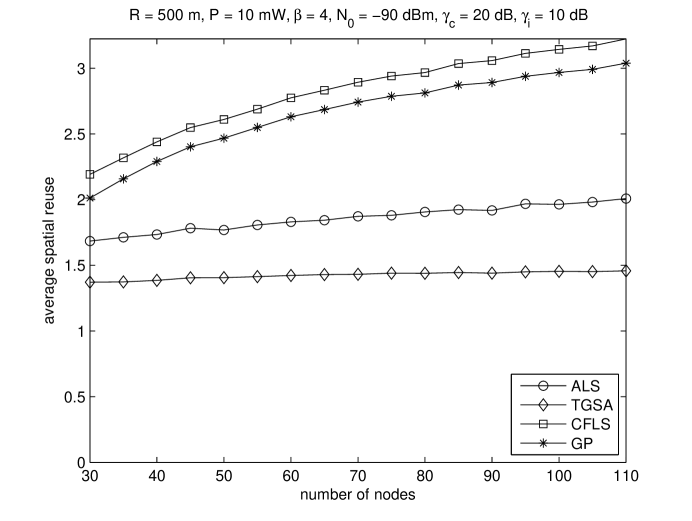
Figure 3.3: Spatial reuse vs. number of nodes for Experiment 1.

In the second set of experiments (Experiment 2), we assume that $R=700$ m, $P=15$ mW, $\beta=4$, $N_{0}=-85$ dBm, $\gamma_{c}=15$ dB and $\gamma_{i}=7$ dB. Thus, $R_{c}=110.7$ m and $R_{i}=175.4$ m. We vary the number of nodes from 70 to 150 in steps of 5. Figure 3.4 plots the average spatial reuse vs. number of nodes for all the algorithms.

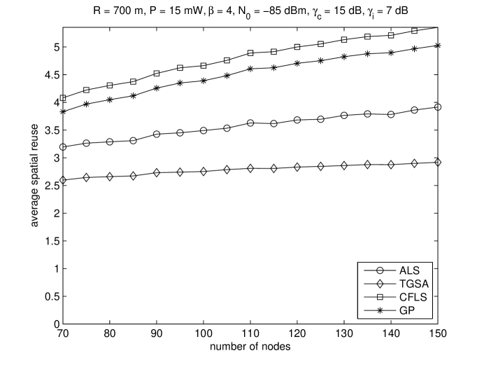
Figure 3.4: Spatial reuse vs. number of nodes for Experiment 2.

For the ALS algorithm, we observe that spatial reuse increases very slowly with increasing number of nodes.

For the TGSA algorithm, we observe that spatial reuse is $18$-$27\%$ lower than that of ALS and $30$-$55\%$ lower than that of GP. A plausible explanation for this behavior is as follows. The basis for TGSA is the computation of $M^{*}$, the optimal number of transmissions in every slot [32]. $M^{*}$ is determined by maximizing a lower bound on the expected number of successful transmissions in a time slot. Since the partitioning of a maximal independent set of communication arcs into subsets of cardinality at most $M^{*}$ is arbitrary and not geography-based, there could be scenarios where the transmissions scheduled in a subset are in the vicinity of each other, resulting in moderate to high interference. In essence, maximizing this lower bound does not necessarily translate to maximizing the number of successful transmissions in a time slot. Also, due to its design, the TGSA algorithm yields higher number of colors compared to ALS and GP.

Though the GP algorithm is based on communication graph and SINR conditions, it yields slightly lower spatial reuse than CFLS. A possible reason for this observation is as follows. The GP algorithm colors edges of the communication graph in the decreasing order of interference number. The interference number of edge $e$ is the number of edges $e_{i}$ such that, if $(e,e_{i})$ are scheduled simultaneously, then the SINR threshold condition (2.7) is violated along one or both links. Edges with higher interference number tend to be located towards the center of the deployment region. Since these edges are colored first, a large number of colors are utilized in the initial stages of the algorithm, lead to potentially higher schedule length and lower spatial reuse. A better technique would be successively examine edges at the centre and the periphery, which is achieved by the partition technique employed by CFLS.

For the proposed CFLS algorithm, we observe that spatial reuse increases steadily with increasing number of nodes and is about $15\%$ higher than the spatial reuse of ALS, TGSA and GP.

Performance Comparison under Realistic Conditions

In a realistic wireless environment, channel impairments like multipath fading and shadowing affect the received SINR at a receiver [14]. In this section, we compare the performance of the ALS, TGSA, GP and CFLS algorithms in a wireless channel which experiences Rayleigh fading and lognormal shadowing.

In the absence of fading and shadowing, the SINR at receiver $r_{i,j}$ is given by (2.2). We assume that every algorithm (ALS, TGSA, GP and CFLS) considers only path loss in the channel prior to constructing the two-tier graph ${\mathcal{G}}({\mathcal{V}},{\mathcal{E}}_{c}\,\cup\,{\mathcal{E}}_{i})$ and computing the link schedule.

However, for computing the average spatial reuse of each algorithm, we take into account fading and shadowing channel gains between each pair of nodes. More specifically, for computing the spatial reuse using (2.14), the (actual) SINR at receiver $r_{i,j}$ is given by

$${\mbox{SINR}}_{r_{i,j}}=\frac{\frac{P}{D^{\beta}(t_{i,j},r_{i,j})}V(t_{i,j},r_{i,j})10^{W(t_{i,j},r_{i,j})}}{N_{0}+\sum_{\stackrel{{\scriptstyle k=1}}{{k\neq j}}}^{M_{i}}\frac{P}{D^{\beta}(t_{i,k},r_{i,j})}V(t_{i,k},r_{i,j})10^{W(t_{i,k},r_{i,j})}},$$ (3.3)

where random variables $V(\cdot)$ and $W(\cdot)$ correspond to channel gains due to Rayleigh fading and lognormal shadowing respectively. We assume that $\{V(k,l)|1\leqslant k,l\leqslant N,k\neq l\}$ are independent and identically distributed (i.i.d.) random variables with probability density function (pdf) [10]

$$f_{V}(v) = \frac{1}{\sigma_{V}^{2}}e^{\frac{-v}{\sigma_{V}^{2}}}u(v),$$ (3.4)

where $u(\cdot)$ is the unit step function. Also, $\{W(k,l)|1\leqslant k,l\leqslant N,k\neq l\}$ are assumed to be i.i.d. zero mean Gaussian random variables with pdf [57]

$$f_{W}(w) = \frac{1}{\sqrt{2\pi}\sigma_{W}}e^{\frac{-w^{2}}{2\sigma_{W}^{2}}}.$$ (3.5)

Random variables $V(\cdot)$ and $W(\cdot)$ are independent of each other and also independent of the node locations.

The simulation model and experiments are exactly as described before. In the simulations, we assume $\sigma_{V}^{2}=\sigma_{W}^{2}=1$. For Experiment 1, Figure 3.5 plots the average spatial reuse vs. number of nodes for all the algorithms. For Experiment 2, Figure 3.6 plots the average spatial reuse vs. number of nodes for all the algorithms.

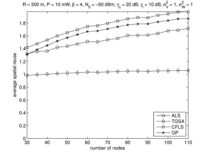
Figure 3.5: Spatial reuse vs. number of nodes for Experiment 1 under multipath fading and shadowing channel conditions.

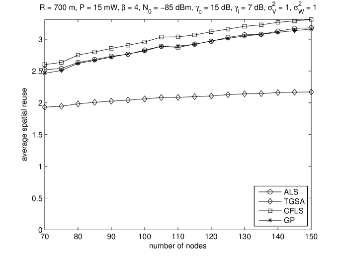
Figure 3.6: Spatial reuse vs. number of nodes for Experiment 2 under multipath fading and shadowing channel conditions.

From Figures 3.3, 3.4, 3.5 and 3.6, we observe that spatial reuse decreases by $20$-$40\%$ in a channel experiencing multipath fading and shadowing effects. A plausible explanation for this observation is as follows. Since the channel gains between every pair of nodes are independent of each other, it is reasonable to assume that the interference power at a typical receiver remains almost the same as in the non-fading case. This is because, even if the power received from few unintended transmitters is low, the power received from other unintended transmitters will be high (on average); thus the interference power remains constant. Consequently, the change in SINR is determined by the change in received signal power only. If the received signal power is higher compared to the non-fading case, the transmission is anyway successful and spatial reuse remains unchanged (see (2.14)). However, if the received signal power is lower, the transmission is now unsuccessful and spatial reuse decreases. Hence, on average, the spatial reuse decreases.

Finally, from Figures 3.5 and 3.6, we observe that the proposed CFLS algorithm achieves $5$-$17\%$ higher spatial reuse than the ALS and GP algorithms and $40$-$80\%$ higher spatial reuse than the TGSA algorithm, under realistic wireless channel conditions.

3.2.5 Analytical Results

In this section, we derive upper bounds on the running time (computational) complexity of ConflictFreeLinkSchedule algorithm. We use the following notation with respect to the communication graph ${\mathcal{G}}_{c}({\mathcal{V}},{\mathcal{E}}_{c})$:

$$e = \mbox{number of communication edges},$$

$$v = \mbox{number of vertices},$$

$$\theta =$$ thickness of the graph

$$:= {\mathcal{G}}_{c}(\cdot)$$ minimum number of planar graphs into which the undirected equivalent of

$$\mbox{can be partitioned}.$$

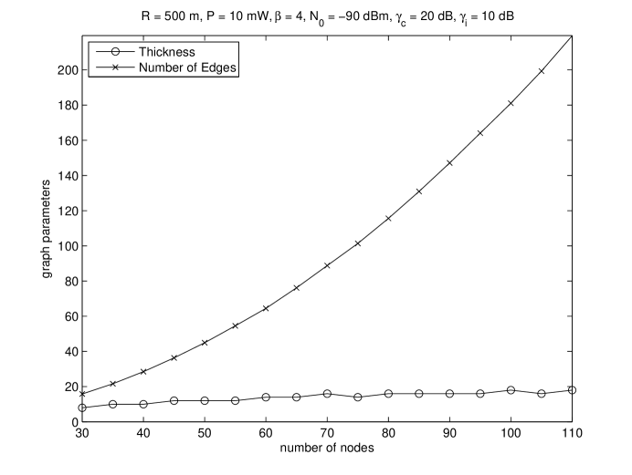
(a) Experiment 1

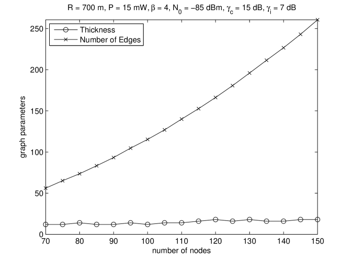
(b) Experiment 2

Figure 3.7: Comparison of thickness and number of edges with number of vertices.

Before we prove our results, it is instructive to observe Figure 3.7, which shows the variation of $\theta$ and $e$ with $v$ for the two experiments described in Section 3.2.4. Since determining the thickness of a graph is NP-hard [58], each value of $\theta$ in Figure 3.7 is an upper bound on the actual thickness based on the number of forests into which the undirected equivalent of the communication graph has been decomposed using successive breadth first searches. We observe that the graph thickness increases very slowly with the number of vertices $(\theta\ll v)$, while the number of edges increases super-linearly with the number of vertices.

Lemma 3.2.1.

An oriented graph $T$ can be colored using no more than $O(v)$ colors using ConflictFreeLinkSchedule.

Proof.

Since an oriented graph with $v$ vertices has at most $v$ edges, the edges of $T$ can be colored with at most $v$ colors. ∎

Lemma 3.2.2.

For an oriented graph $T$, the running time of ConflictFreeLinkSchedule is $O(v^{2})$.

Proof.

Assuming that an element can be chosen randomly and uniformly from a finite set in unit time ([53], Chapter 1), the running time of Phase 1 can be shown to be $O(v)$. Since there is only one oriented graph, Phase 2 runs in time $O(v)$. In Phase 3, the unique edge associated with the vertex under consideration is assigned a color using FirstConflictFreeColor. From Lemma 3.2.1, the size of the set of colors to be examined $|{\mathcal{C}}_{c}\cup{\mathcal{C}}_{cf}|$ is $O(v)$. In FirstConflictFreeColor, the SINR is checked only once for every colored edge in the set $\bigcup_{i=1}^{|{\mathcal{C}}_{cf}|}E_{i}$ and at most $v$ times for the edge under consideration $x$. With a careful implementation, FirstConflictFreeColor runs in time $O(v)$. So, the running time of Phase 3 is $O(v^{2})$. Thus, the total running time is $O(v^{2})$. ∎

Theorem 3.2.3.

For an arbitrary graph $\mathcal{G}$, the running time of ConflictFreeLinkSchedule is $O(ev\log v+ev\theta)$.

Proof.

Assuming that an element can be chosen randomly and uniformly from a finite set in unit time [53], the running time of Phase 1 can be shown to be $O(v)$. For Phase 2, the optimal partitioning technique of [49] based on Matroids can be used to partition the communication graph ${\mathcal{G}}_{c}$ into at most $6\theta$ oriented graphs in time $O(ev\log v)$. Thus, $k\leqslant 6\theta$ holds for Phase 3. From Lemma 3.2.2, it follows that the first oriented graph $T_{1}$ can be colored in time $O(v^{2})$. However, consider the coloring of $j^{th}$ oriented graph $T_{j}$, where $2\leqslant j\leqslant k$. When coloring edge $x$ from $T_{j}$ using FirstConflictFreeColor, conflicts can occur not only with the colored edges of $T_{j}$, but also with the edges of the previously colored oriented graphs $T_{1},T_{2},\ldots,T_{j-1}$. Hence, the worst-case size of the set of colors to be examined $|{\mathcal{C}}_{c}\cup{\mathcal{C}}_{cf}|$ is $O(e)$. Note that in FirstConflictFreeColor, the SINR is checked only once for every colored edge in the set $\bigcup_{i=1}^{|{\mathcal{C}}_{cf}|}E_{i}$ and at most $e$ times for the edge under consideration $x$. With a careful implementation, FirstConflictFreeColor runs in time $O(e)$. Hence, any subsequent oriented graph $T_{j}$ can be colored in time $O(ev)$. Thus, the running time of Phase 3 is $O(ev\theta)$. Therefore, the overall running time of ConflictFreeLinkSchedule is $O(ev\log v+ev\theta)$. ∎

3.2.6 Discussion

In this section, we have developed ConflictFreeLinkSchedule, a point to point link scheduling algorithm for an STDMA wireless mesh network under the physical interference model. The performance of the proposed algorithm is superior to those of existing link scheduling algorithms for STDMA wireless networks with uniform power assignment. A practical experimental modeling shows that, on average, the proposed algorithm achieves $20\%$ higher spatial reuse than the ArboricalLinkSchedule [16], GreedyPhysical [27] and Truncated Graph-Based Scheduling [32] algorithms. Since link schedules are constructed offline only once and then used by the network for a long period of time, these improvements in performance directly translate to higher long-term network throughput.

The computational complexity of ConflictFreeLinkSchedule is comparable to the computational complexity of ArboricalLinkSchedule and is much lower than the computational complexity of GreedyPhysical and Truncated Graph-Based Scheduling algorithms. Thus, in cognizance of spatial reuse as well as computational complexity, ConflictFreeLinkSchedule appears to be a good candidate for efficient STDMA link scheduling algorithms.

Chapter 4 Point to Point Link Scheduling based on SINR Graph Model

In this chapter, we propound a somewhat different approach for point to point link scheduling in an STDMA wireless network under the physical interference model. This approach is based on SINR graph representation of the network wherein weights of edges correspond to interferences between pairs of nodes and weights of vertices correspond to normalized noise powers at receiving nodes. We develop a novel link scheduling algorithm with polynomial time complexity and improved performance in terms of spatial reuse.

The rest of the chapter is organized as follows. We motivate our SINR graph approach in Section 4.1. We describe the proposed link scheduling algorithm and provide an illustrative example in Section 4.2. We prove the correctness of the algorithm and derive its computational complexity in Section 4.3. The performance of the proposed algorithm is compared with existing link scheduling algorithms in Section 4.4. We discuss the implications of our work in Section 4.5.

4.1 Motivation

The system model, notation and problem formulation are exactly as described in Section 3.2.1. Specifically, we seek a low complexity conflict-free point to point link scheduling algorithm that achieves high spatial reuse.

In general, for the STDMA wireless network $\Phi(\cdot)$, the set of links to be scheduled is determined by a routing algorithm. For simplicity, we only consider exhaustive link schedules, i.e., we consider uniform load on all links.

Note that for point to point link schedules that are conflict-free, i.e., for link schedules that satisfy (2.7), the equation for spatial reuse (2.14) reduces to

Spatial Reuse $$= \sigma\;=\;\frac{e}{C},$$ (4.1)

where $e$ denotes the number of directed edges in the communication graph $\mathcal{G}_{c}(\mathcal{V},\mathcal{E}_{c})$ and $C$ denotes the number of slots in the link schedule. Therefore, for conflict-free link schedules, maximizing spatial reuse is equivalent to minimizing the number of colors, i.e., minimizing the schedule length.

To the best of our knowledge, there is no known polynomial time algorithm that determines a provably optimal schedule (minimum length schedule) for an STDMA wireless network with constrained transmission power. Hence, the only recourse is to devise heuristics and show their efficiency theoretically and experimentally. Towards this end, we propose a heuristic based on an SINR graph representation of the network.

Consider any directed graph $G(V,E)$, where $V$ is the set of vertices and $E$ is the set of edges. The line graph of $G(V,E)$ is the graph $G^{\prime}(V^{\prime},E^{\prime})$ whose vertices are the edges of $G(\cdot)$, i.e., $V^{\prime}=E$ [35]. The SINR graph that we consider in this chapter is analogous to the concept of line graph in [35]. However, unlike the line graph, we assume that the SINR graph is a complete graph, i.e., for any two distinct vertices $v_{i}^{\prime}$, $v_{j}^{\prime}$ $\in V^{\prime}$, there is a directed edge from $v_{i}^{\prime}$ to $v_{j}^{\prime}$ in $E^{\prime}$.

The crux of the proposed link scheduling algorithm can be understood by revisiting the condition for successful packet reception under the physical interference model (Equation 2.6), i.e.,

$$\frac{\frac{P}{D^{\beta}(t_{i,j},r_{i,j})}}{N_{0}+\sum_{\stackrel{{\scriptstyle k=1}}{{k\neq j}}}^{M_{i}}\frac{P}{D^{\beta}(t_{i,k},r_{i,j})}}\geqslant\gamma_{c}.$$ (4.2)

Rearranging the terms in (4.2), we obtain

$$\frac{N_{0}\gamma_{c}}{P}D^{\beta}(t_{i,j},r_{i,j})+\sum_{\stackrel{{\scriptstyle k=1}}{{k\neq j}}}^{M_{i}}\gamma_{c}\frac{D^{\beta}(t_{i,j},r_{i,j})}{D^{\beta}(t_{i,k},r_{i,j})} \leqslant 1.$$ (4.3)

Dropping time slot index $i$ for clarity, we obtain the “equivalent” SINR threshold condition

$$\frac{N_{0}\gamma_{c}}{P}D^{\beta}(t_{j},r_{j})+\sum_{\stackrel{{\scriptstyle k=1}}{{k\neq j}}}^{M}\gamma_{c}\frac{D^{\beta}(t_{j},r_{j})}{D^{\beta}(t_{k},r_{j})} \leqslant 1,$$ (4.4)

where $t_{j}$, $r_{j}$ and $M$ can be interpreted as $j^{th}$ transmitter, $j^{th}$ receiver and number of concurrent transmissions, respectively, in a given time slot. The terms appearing in (4.4) correspond to vertex and edge weights in a special graph representation of the STDMA network, termed as SINR graph. This idea will be elucidated further in Section 4.2.1.

4.2 SINRGraphLinkSchedule Algorithm

In this section, we explain the proposed link scheduling algorithm based on SINR graph representation of the STDMA network. We provide an illustrative example to elucidate the intricacies of the proposed algorithm.

4.2.1 Description

Algorithm 6 SINRGraphLinkSchedule (SGLS)

1:  Input: Communication graph ${\mathcal{G}}_{c}$(${\mathcal{V}}$,${\mathcal{E}_{c}}$), $\gamma_{c}$, $N_{0}$, $P$

2:  Output: A coloring ${\mathcal{C}}$: ${\mathcal{E}_{c}}\rightarrow\{1,2,\ldots\}$

3:  ${\mathcal{V}^{\prime}}\leftarrow{\mathcal{E}_{c}}$

4:  Construct the directed complete graph $\mathcal{G}^{\prime}(\mathcal{V}^{\prime},\mathcal{E}^{\prime})$

5:  for all $e^{\prime}_{ij}\in{\mathcal{E}^{\prime}}$ do

6:     if edges $i$ and $j$ have a common vertex in $\mathcal{G}_{c}(\cdot)$ then

7:        $w_{ij}\leftarrow 1$

8:     else

9:        $w_{ij}\leftarrow\gamma_{c}\frac{{D(t_{j},r_{j})}^{\beta}}{{D(t_{i},r_{j})}^{\beta}}$

10:     end if

11:  end for

12:  for all $e^{\prime}_{ij}\in{\mathcal{E}^{\prime}}$ do

13:     $w^{\prime}_{ij}\leftarrow\max\{0,1-w_{ij}\}$

14:  end for

15:  for all $v_{j}^{\prime}\in{\mathcal{V}^{\prime}}$ do

16:     ${\mathcal{N}}(v_{j}^{\prime})\leftarrow\frac{N_{0}\gamma_{c}}{P}{{D(t_{j},r_{j})}^{\beta}}$

17:  end for

18:  $p\leftarrow 0$; ${\mathcal{V}_{uc}^{\prime}}\leftarrow{\mathcal{V}^{\prime}}$

19:  while ${\mathcal{V}_{uc}^{\prime}}\neq\phi$ do

20:     $p\leftarrow p+1$; choose $v^{\prime}\in\mathcal{V}_{uc}^{\prime}$ randomly

21:     ${\mathcal{C}}(v^{\prime})\leftarrow p$; ${\mathcal{V}_{uc}^{\prime}}\leftarrow{\mathcal{V}_{uc}^{\prime}}\setminus\{v^{\prime}\}$; ${\mathcal{V}_{c_{p}}^{\prime}}\leftarrow\{v^{\prime}\}$; $\psi\leftarrow\mbox{1}$

22:     while $\psi=1$ and $\mathcal{V}_{uc}^{\prime}\neq\phi$ and $\max_{y^{\prime}\in{\mathcal{V}}_{uc}^{\prime}}\sum_{x^{\prime}\in{\mathcal{V}}_{c_{p}}^{\prime}}w^{\prime}_{x^{\prime}y^{\prime}}+w^{\prime}_{y^{\prime}x^{\prime}}>0$ do

23:        for all $u^{\prime}\in\mathcal{V}_{uc}^{\prime}$ such that $\sum_{x^{\prime}\in{\mathcal{V}}_{c_{p}}^{\prime}}w^{\prime}_{x^{\prime}u^{\prime}}+w^{\prime}_{u^{\prime}x^{\prime}}>0$ do

24:           $\varrho\leftarrow 1$

25:           for all $v_{c}^{\prime}\in{\mathcal{V}_{c_{p}}^{\prime}}$ do

26:              if $\sum_{v_{1}^{\prime}\in{\mathcal{V}_{c_{p}}^{\prime}}\setminus\{v_{c}^{\prime}\}\cup\{u^{\prime}\}}w^{\prime}_{{v_{1}^{\prime}}{v_{c}^{\prime}}}\leqslant|{\mathcal{V}_{c_{p}}^{\prime}}|+{\mathcal{N}}(v_{c}^{\prime})-1$ then

27:                 $\varrho\leftarrow 0$

28:              end if

29:           end for

30:           if $\varrho=1$ and $\sum_{v_{2}^{\prime}\in{\mathcal{V}_{c_{p}}^{\prime}}}w^{\prime}_{{v_{2}^{\prime}}u^{\prime}}>|{\mathcal{V}_{c_{p}}^{\prime}}|+{\mathcal{N}}(u^{\prime})-1$ then

31:              ${\mathcal{C}}(u^{\prime})\leftarrow p$; ${\mathcal{V}_{c_{p}}^{\prime}}\leftarrow{\mathcal{V}_{c_{p}}^{\prime}}\cup\{u^{\prime}\}$; ${\mathcal{V}_{uc}^{\prime}}\leftarrow{\mathcal{V}_{uc}^{\prime}}\setminus\{u^{\prime}\}$

32:           else

33:              $\varrho\leftarrow 0$

34:           end if

35:        end for

36:        if $\varrho=0$ then

37:           $\psi\leftarrow 0$

38:        end if

39:     end while

40:  end while

The proposed link scheduling algorithm under the physical interference model is SINRGraphLinkSchedule (SGLS), which considers the communication graph $\mathcal{G}_{c}(\mathcal{V},\mathcal{E}_{c})$.

First, we construct a directed complete SINR graph ${\mathcal{G}^{\prime}}({\mathcal{V}^{\prime}},{\mathcal{E}^{\prime}})$ that has the edges of $\mathcal{G}_{c}(\cdot)$ as its vertices, i.e., $\mathcal{V}^{\prime}=\mathcal{E}_{c}$. Let the edges of $\mathcal{G}_{c}(\cdot)$ and the corresponding vertices of $\mathcal{G}^{\prime}(\cdot)$ be labeled $1,2,\ldots,e$. Let $t_{i}$ and $r_{i}$ denote the transmitter and receiver respectively of edge $i$ in $\mathcal{G}_{c}(\cdot)$. For any two edges $i$ and $j$ in graph $\mathcal{G}_{c}(\cdot)$, the interference weight function $w_{ij}$ is defined as:

$$w_{ij} := \left\{\begin{array}[]{ll}1&\mbox{if $i$ and $j$ have a common vertex},\\ \gamma_{c}\frac{D(t_{j},r_{j})^{\beta}}{D(t_{i},r_{j})^{\beta}}&\mbox{otherwise}.\end{array}\right.$$

The interference weight function $w_{ij}$ indicates the interference energy at $r_{j}$ due to transmission from $t_{i}$ to $r_{i}$ scaled with respect to the signal energy of $t_{j}$ at $r_{j}$. Note that the interference weight function appears as a summand in the equivalent SINR threshold condition (4.4).

We then compute the co-schedulability weight function $w^{\prime}$. For any two edges $i$ and $j$ in $\mathcal{G}_{c}(\cdot)$, the weight of edge $e^{\prime}_{ij}$ in ${\mathcal{G}^{\prime}}(\cdot)$ is given by $w^{\prime}_{ij}=\max\{0,1-w_{ij}\}$. Since $w_{ij}$ and $w_{ji}$ represent interferences among links $i$ and $j$ in the STDMA network $\Phi(\cdot)$, $w^{\prime}_{ij}$ and $w^{\prime}_{ji}$ intuitively represent the co-schedulability of links $i$ and $j$ in $\Phi(\cdot)$ (equivalently, co-schedulability of vertices $i$ and $j$ in $\mathcal{G}^{\prime}(\cdot)$). For example, if $w_{ij}$ is greater than or equal to $1$, then the interference at the receiver of link $j$ from the transmitter of link $i$ is very high and these links cannot be scheduled simultaneously. This will result in $w^{\prime}_{ij}$ being equal to $0$ indicating that vertices $i$ and $j$ in $\mathcal{G}^{\prime}(\cdot)$ are not co-schedulable. On the other hand, if $w_{ij}$ is slightly greater than $0$ $(0<w_{ij}\ll 1)$, $w^{\prime}_{ij}$ will be slightly less than $1$ indicating that the vertices $i$ and $j$ in $\mathcal{G}^{\prime}(\cdot)$ are co-schedulable. Note that for the SINR graph $\mathcal{G}^{\prime}(\cdot)$, the weight of an edge refers to the value of co-schedulability function for that edge.

Next, we determine the normalized noise power at the receiver of each link of $\Phi(\cdot)$. This is tantamount to computing the normalized noise power for each edge of $\mathcal{G}_{c}(\cdot)$, i.e., at each vertex of ${\mathcal{G}^{\prime}}(\cdot)$. Note that the normalized noise power function appears as a term in the equivalent SINR threshold condition (4.4).

Our objective is to color the vertices of ${\mathcal{G}^{\prime}}(\cdot)$ (equivalently, edges of $\mathcal{G}_{c}(\cdot)$) using minimum number of colors under the physical interference model, i.e., subject to the condition that the SINR at the receiver of every link in $\Phi(\cdot)$ is no less than the communication threshold $\gamma_{c}$. Equivalently, for any ${\mathcal{V}_{cc}^{\prime}}\subseteq{\mathcal{V}^{\prime}}$, the coloring of all vertices $v_{i}^{\prime}\in{\mathcal{V}_{cc}^{\prime}}$ with the same color is defined to be feasible if

$$\frac{\frac{P}{{D(t_{v_{i}^{\prime}},r_{v_{i}^{\prime}})}^{\beta}}}{N_{0}+\sum_{v_{j}^{\prime}\in{\mathcal{V}_{cc}^{\prime}}\setminus\{v_{i}^{\prime}\}}\frac{P}{{D(t_{v_{j}^{\prime}},r_{v_{i}^{\prime}})}^{\beta}}}\geqslant\gamma_{c}\;\;\forall\;\;v_{i}^{\prime}\in{\mathcal{V}_{cc}^{\prime}}.$$ (4.6)

In the SINR graph $\mathcal{G}^{\prime}(\cdot)$, this condition translates to the sum of weights of edges incoming to a vertex from all co-colored vertices being greater than the sum of the number of remaining co-colored vertices and the normalized noise power minus a constant factor (unity); this will be proved in Theorem 4.3.1.

Finally, we color vertices of $\mathcal{G}^{\prime}(\cdot)$, i.e., edges of $\mathcal{G}_{c}(\cdot)$, according to the following procedure. Let ${\mathcal{V}_{uc}^{\prime}}$ denote the set of uncolored vertices of $\mathcal{G}^{\prime}(\cdot)$. Initially, $\mathcal{V}_{uc}^{\prime}$ includes all vertices of $\mathcal{G}^{\prime}(\cdot)$. First, we choose a vertex randomly from ${\mathcal{V}_{uc}^{\prime}}$. This is assigned a new color, say $p$. Then, we consider every vertex $u^{\prime}$ from ${\mathcal{V}_{uc}^{\prime}}$ such that the sum of weights of all the edges between $u^{\prime}$ and the vertices colored with $p$ is positive. Next, for each vertex colored with $p$, we check if the sum of weights of all incoming edges is greater than the sum of the number of vertices colored with $p$ and the normalized noise power at that vertex minus a constant factor (unity). If this inequality is satisfied, we further check if the sum of weights of all edges incoming to $u$ is greater than the sum of the number of vertices colored with $p$ and the normalized noise power at $u^{\prime}$ minus unity. If this inequality is also satisfied, then vertex $u^{\prime}$ is colored with $p$. If any of these inequalities are not satisfied, vertex $u^{\prime}$ is colored with a new color. The algorithm exits when all the vertices are colored. The pseudocode of the algorithm is provided in Algorithm 6.

4.2.2 Example

Consider the STDMA wireless network $\Phi(\cdot)$ whose deployment is shown in Figure 4.1. It consists of four labeled nodes whose coordinates (in meters) are $1\equiv(-40,5)$, $2\equiv(0,0)$, $3\equiv(95,0)$ and $4\equiv(135,0)$. We use typical values of system parameters in wireless networks [42]. These values are shown in Table 4.1, which lead to $R_{c}=100$ m.

Figure 4.1: An STDMA wireless network with four nodes.

Parameter	Symbol	Value
transmission power	$P$	10 mW
path loss exponent	$\beta$	4
noise power spectral density	$N_{0}$	-90 dBm
communication threshold	$\gamma_{c}$	20 dB

Table 4.1: System parameters for the STDMA network shown in Figure 4.1.

The communication graph model of the STDMA network is shown in Figure 4.2. The communication graph $\mathcal{G}_{c}(\mathcal{V},\mathcal{E}_{c})$ consists of four vertices and six directed edges. The vertex and edge sets are given by

$$\mathcal{V} = \{v_{1},v_{2},v_{3},v_{4}\},$$ (4.7)

$$\mathcal{E}_{c} = \{(1,2),(2,1),(2,3),(3,2),(3,4),(4,3)\}.$$ (4.8)

Figure 4.2: Communication graph model of STDMA network described by Figure 4.1 and Table 4.1.

The SINR graph model of the communication graph $\mathcal{G}_{c}(\mathcal{V},\mathcal{E}_{c})$ is shown in Figure 4.3. The SINR graph $\mathcal{G}^{\prime}(\mathcal{V}^{\prime},\mathcal{E}^{\prime})$ is a complete graph and consists of six vertices and thirty directed edges. The vertex set of the SINR graph is given by

$$\mathcal{V}^{\prime} = \{(1,2),(2,1),(2,3),(3,2),(3,4),(4,3)\}.$$ (4.9)

The edge set $\mathcal{E}^{\prime}$ of the SINR graph is enumerated in Table 4.2, along with the interference weight function $w_{ij}$ and co-schedulability weight function $w_{ij}^{\prime}$ for each edge $i\rightarrow j\in\mathcal{G}^{\prime}(\cdot)$. The normalized noise powers at vertices of the SINR graph are enumerated in Table 4.3.

Figure 4.3: SINR graph model of communication graph shown in Figure 4.2.

Edge $i\rightarrow j$ of			Edge $i\rightarrow j$ of
SINR graph $\mathcal{G}^{\prime}(\mathcal{V}^{\prime},\mathcal{E}^{\prime})$	$w_{ij}$	$w_{ij}^{\prime}$	SINR graph $\mathcal{G}^{\prime}(\mathcal{V}^{\prime},\mathcal{E}^{\prime})$	$w_{ij}$	$w_{ij}^{\prime}$
$(1,2)\rightarrow(2,1)$	1	0	$(3,2)\rightarrow(1,2)$	1	0
$(2,1)\rightarrow(1,2)$	1	0	$(1,2)\rightarrow(3,4)$	0.2725	0.7275
$(2,1)\rightarrow(2,3)$	1	0	$(3,4)\rightarrow(1,2)$	3.2420	0
$(2,3)\rightarrow(2,1)$	1	0	$(2,1)\rightarrow(3,2)$	1	0
$(2,3)\rightarrow(3,2)$	1	0	$(3,2)\rightarrow(2,1)$	1	0
$(3,2)\rightarrow(2,3)$	1	0	$(2,1)\rightarrow(3,4)$	0.7707	0.2293
$(3,2)\rightarrow(3,4)$	1	0	$(3,4)\rightarrow(2,1)$	0.7928	0.2072
$(3,4)\rightarrow(3,2)$	1	0	$(2,1)\rightarrow(4,3)$	3.1430	0
$(3,4)\rightarrow(4,3)$	1	0	$(4,3)\rightarrow(2,1)$	0.2811	0.7189
$(4,3)\rightarrow(3,4)$	1	0	$(2,3)\rightarrow(3,4)$	1	0
$(4,3)\rightarrow(1,2)$	0.7950	0.2050	$(3,4)\rightarrow(2,3)$	1	0
$(1,2)\rightarrow(4,3)$	0.7686	0.2314	$(2,3)\rightarrow(4,3)$	1	0
$(1,2)\rightarrow(2,3)$	1	0	$(4,3)\rightarrow(2,3)$	1	0
$(2,3)\rightarrow(1,2)$	1	0	$(3,2)\rightarrow(4,3)$	1	0
$(1,2)\rightarrow(3,2)$	1	0	$(4,3)\rightarrow(3,2)$	1	0

Table 4.2: Interference and co-schedulability weight functions for edges of SINR graph shown in Figure 4.3.

Vertex $v_{j}^{\prime}$ of
SINR graph $\mathcal{G}^{\prime}(\mathcal{V}^{\prime},\mathcal{E}^{\prime})$	$\mathcal{N}(v_{j}^{\prime})$
(1,2)	0.0264
(2,1)	0.0264
(2,3)	0.8145
(3,2)	0.8145
(3,4)	0.0256
(4,3)	0.0256

Table 4.3: Normalized noise powers at vertices of SINR graph shown in Figure 4.3.

The truncated SINR graph $\mathcal{G}_{t}^{\prime}(\mathcal{V}^{\prime},\mathcal{E}_{t}^{\prime})$ is shown in Figure 4.4. The truncated SINR graph consists of all vertices of the SINR graph and only those edges whose co-schedulability weight function is positive, i.e., $\mathcal{E}_{t}^{\prime}=\{(i,j):i,j\in\mathcal{E}_{c}\mbox{ and }w_{ij}^{\prime}>0\}$. The values of the co-schedulability weight functions for all edges and the normalized noise powers at all vertices are also shown in the figure. We use the truncated SINR graph to explain the SGLS algorithm, since edges having zero weight in the SINR graph do not play any role in the SGLS algorithm. Note that, in the truncated SINR graph, the weight of an edge refers to the value of the co-schedulability weight function for that edge.

Figure 4.4: Truncated SINR graph derived from SINR graph shown in Figure 4.3 and weight values given in Tables 4.2 and 4.3.

Initially, the set of uncolored vertices is $\mathcal{V}_{uc}^{\prime}=\{(1,2),(2,1),(2,3),(3,2),(3,4),(4,3)\}$. In the first iteration, we randomly choose $v^{\prime}=(1,2)$ and assign it Color $1$ (say, red). So, $\mathcal{C}(1,2)=1$. The set of uncolored vertices is $\mathcal{V}_{uc}^{\prime}=\{(2,1),(2,3),(3,2),(3,4),(4,3)\}$ and the set of vertices colored 1 is $\mathcal{V}_{c_{1}}^{\prime}=\{(1,2)\}$. From the set of uncolored vertices $\mathcal{V}_{uc}^{\prime}$, we consider every vertex $u^{\prime}$ such that the sum of weights of edges from the presently colored vertex $(1,2)$ to $u^{\prime}$ and from $u^{\prime}$ to the presently colored vertex is positive. From Figure 4.4, we obtain two candidates: $u^{\prime}=(3,4)$ and $u^{\prime}=(4,3)$. We first examine the candidate vertex $(3,4)$. We check if the weight of the edge from $(3,4)$ to the presently colored vertex $(1,2)$ is no greater than the number of vertices colored with the present color (red) plus the normalized noise power at the colored vertex minus unity. Our calculations show that inequality holds $(0<0.0264)$ and candidate vertex $(3,4)$ cannot be assigned Color 1. We next examine the candidate vertex $(4,3)$. We check if the weight of the edge from the candidate vertex to $(1,2)$ is no greater than the number of vertices colored with the present color plus the normalized noise power at $(1,2)$ minus unity. Our calculations show that inequality does not hold $(0.2050\not\leqslant 0.0264)$. Furthermore, we check if the weight of the edge from the presently colored vertex $(1,2)$ to the candidate vertex $(4,3)$ is greater than the number of vertices colored red plus the normalized noise power at $(4,3)$ minus unity. The inequality holds and hence the candidate vertex $(4,3)$ is assigned Color 1 (red). So, $\mathcal{C}(4,3)=1$. The set of uncolored vertices is $\mathcal{V}_{uc}^{\prime}=\{(2,1),(2,3),(3,2),(3,4)\}$ and the set of vertices colored 1 is $\mathcal{V}_{c_{1}}^{\prime}=\{(1,2),(4,3)\}$. Again, from the set of uncolored vertices $\mathcal{V}_{uc}^{\prime}$, we consider every vertex $u^{\prime}$ such that the sum of weights of edges from the presently colored vertices $\{(1,2),(4,3)\}$ to $u^{\prime}$ and from $u^{\prime}$ to the presently colored vertices is positive. From Figure 4.4, the candidate vertices are $(2,1)$ and $(3,4)$. Consider the candidate vertex $(2,1)$. For every vertex $v_{c}^{\prime}$ colored 1, we check if the sum of weights of edges from remaining co-colored vertices and the candidate vertex to the colored vertex is no greater than the number of co-colored vertices and the normalized noise power at the colored vertex minus unity. For the colored vertex $(1,2)$, our calculations show that inequality holds $(0.2050\leqslant 1.0264)$. So, we discard $(2,1)$, consider the next candidate vertex $(3,4)$ and perform an analogous comparison with $v_{c}^{\prime}=(1,2)$. Since inequality holds in this case too $(0.2050\leqslant 1.0264)$, we discard $(3,4)$ and proceed to the next iteration. The set of vertices colored so far is shown in Figure 4.5.

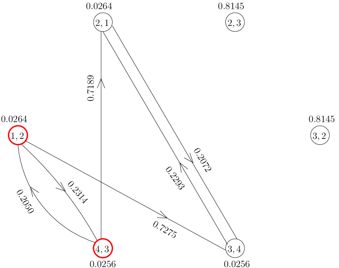
Figure 4.5: Coloring of vertices of truncated SINR graph after first iteration of SGLS algorithm.

In the second iteration, we randomly choose $v^{\prime}=(2,3)$ and assign it Color 2 (say, blue). So, $\mathcal{C}(2,3)=2$. The set of uncolored vertices is $\mathcal{V}_{uc}^{\prime}=\{(2,1),(3,2),(3,4)\}$ and the set of vertices colored 2 is $\mathcal{V}_{c_{2}}^{\prime}=\{(2,3)\}$. From the set of uncolored vertices $\mathcal{V}_{uc}^{\prime}$, we consider every vertex $u^{\prime}$ such that the sum of weights of edges from the presently colored vertex $(2,3)$ to $u^{\prime}$ and from $u^{\prime}$ to the presently colored vertex is positive. From Figure 4.5, no such vertex exists. So, we proceed to the next iteration. The vertices colored so far are shown in Figure 4.6.

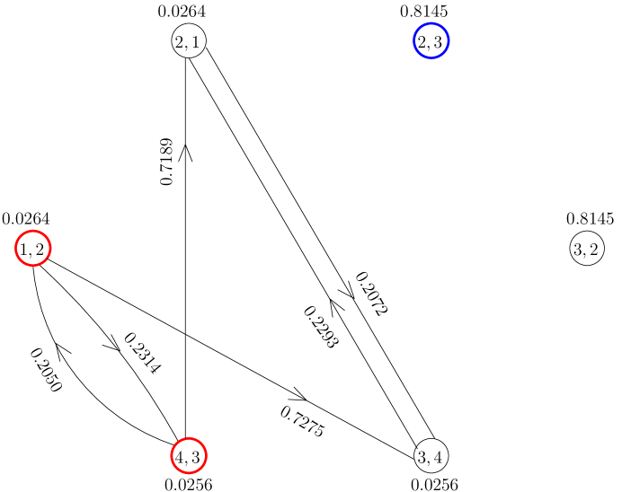
Figure 4.6: Coloring of vertices of truncated SINR graph after second iteration of SGLS algorithm.

In the third iteration, we randomly choose $v^{\prime}=(3,4)$ and assign it Color 3 (say, green). So, $\mathcal{C}(3,4)=3$. The set of uncolored vertices is $\mathcal{V}_{uc}^{\prime}=\{(2,1),(3,2)\}$ and the set of vertices colored 3 is $\mathcal{V}_{c_{3}}^{\prime}=\{(3,4)\}$. From the set of uncolored vertices $\mathcal{V}_{uc}^{\prime}$, we consider every vertex $u^{\prime}$ such that the sum of weights of edges from the presently colored vertex $(3,4)$ to $u^{\prime}$ and from $u^{\prime}$ to the presently colored vertex is positive. From Figure 4.4, we obtain $u^{\prime}=(2,1)$ as the only candidate vertex. Next, we check if the weight of the edge from the candidate vertex $(2,1)$ to the presently colored vertex $(3,4)$ is no greater than the number of vertices colored with the present color (green) plus the normalized noise power at the colored vertex minus unity. Our calculations show that inequality does not hold $(0.2293\not\leqslant 0.0256)$. So, we further check if the weight of the edge from the presently colored vertex $(3,4)$ to the candidate vertex $(2,1)$ exceeds the number of vertices colored with the present color plus the normalized noise power at the candidate vertex minus unity. Since the inequality holds $(0.2072>0.0264)$, the candidate vertex $(2,1)$ is assigned Color 3 (green). So, $\mathcal{C}(2,1)=3$. The set of uncolored vertices is $\mathcal{V}_{uc}^{\prime}=\{(3,2)\}$ and the set of vertices colored green is $\mathcal{V}_{c_{3}}^{\prime}=\{(3,4),(2,1)\}$. Next, from the set of uncolored vertices $\mathcal{V}_{uc}^{\prime}$, we choose that uncolored vertex $u^{\prime}$ such that the sum of weights of edges from $u^{\prime}$ to the set of presently colored vertices $\{(3,4),(2,1)\}$ and from $\{(3,4),(2,1)\}$ to $u^{\prime}$ is positive. From Figure 4.6, no such vertex $u^{\prime}$ exists. So, we proceed to the next iteration. Figure 4.7 shows the set of vertices colored so far.

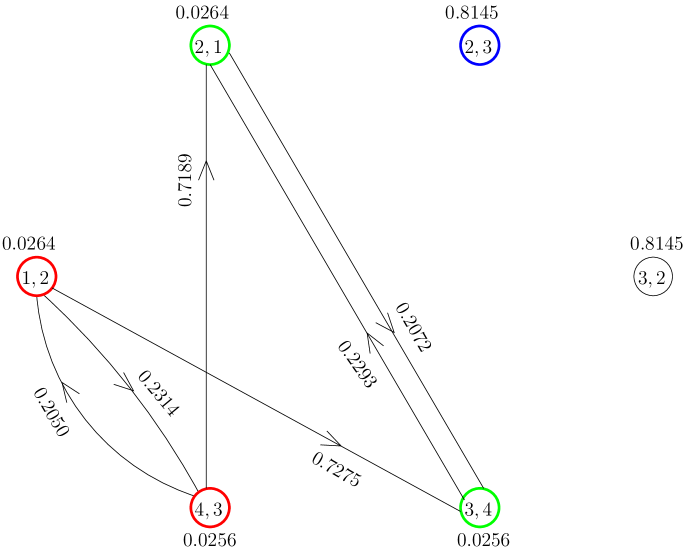
Figure 4.7: Coloring of vertices of truncated SINR graph after third iteration of SGLS algorithm.

In the fourth iteration, $(3,2)$ is the only uncolored vertex. So, we choose $v^{\prime}=(3,2)$ and assign it Color 4 (say, pink). The set of vertices colored 4 is $\mathcal{V}_{c_{4}}^{\prime}=\{(3,2)\}$ and the set of uncolored vertices is $\mathcal{V}_{uc}^{\prime}=\phi$. So, the algorithm ends. The final coloring of vertices of the truncated SINR graph by SGLS algorithm is shown in Figure 4.8.

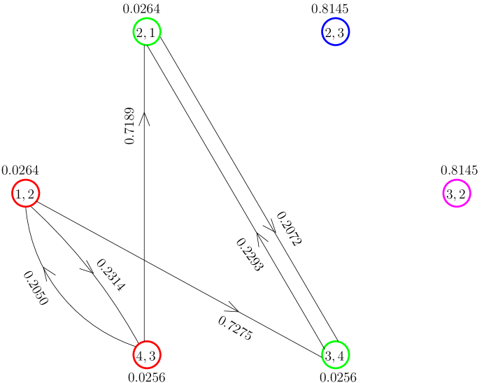
Figure 4.8: Coloring of vertices of truncated SINR graph after complete execution of SGLS algorithm.

The output of the SGLS algorithm is enumerated in Table 4.4 and is also shown pictorially in Figure 4.9. The resulting link schedule is denoted by $\Psi(\mathcal{S}_{1},\mathcal{S}_{2},\mathcal{S}_{3},\mathcal{S}_{4},\mathcal{S}_{5})$, where

$$\mathcal{S}_{1} = \{1\rightarrow 2,\;4\rightarrow 3\},$$

$$\mathcal{S}_{2} = \{2\rightarrow 3\},$$

$$\mathcal{S}_{3} = \{3\rightarrow 4,\;2\rightarrow 1\},$$

$$\mathcal{S}_{4} = \{3\rightarrow 2\}.$$

Time slot	Color	Active (transmitter, receiver) pairs
1	red	(1,2), (4,3)
2	blue	(2,3)
3	green	(3,4), (2,1)
4	pink	(3,2)

Table 4.4: Output of SGLS algorithm for STDMA network described by Figure 4.1 and Table 4.1.

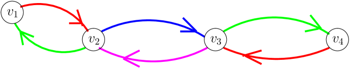
Figure 4.9: Output of SGLS algorithm for STDMA network described by Figure 4.1 and Table 4.1.

Finally, we check if the link schedule enumerated in Table 4.4 is conflict-free, i.e., if the SINR threshold condition (2.7) is satisfied at every receiver for the STDMA network described by Figure 4.1 and Table 4.1. Only one transmitter-receiver pair is active during time slots 2 and 4. Since the receiver is within the communication range of its corresponding transmitter for each of these time slots, the SINR threshold condition is satisfied trivially for time slots 2 and 4. Two transmitter-receiver pairs are active during time slots 1 and 3. In time slot 1, the active transmitter-receiver pairs are $(1,2)$ and $(4,3)$. Our computations show that the SINRs at Receivers 2 and 3 are $20.85$ dB and $21$ dB, both of which exceed the communication threshold of $20$ dB. In time slot 3, the active transmitter-receiver pairs are $(2,1)$ and $(3,4)$. Our computations show that the SINRs at Receivers 1 and 4 are $20.87$ dB and $20.99$ dB respectively, both of which exceed the communication threshold. This verifies that the SGLS algorithm yields a conflict-free link schedule for the network described by Figure 4.1 and Table 4.1. Note that, from (4.1), the spatial reuse of SGLS algorithm for this network is $1.5$.

4.3 Analytical Results

In this section, we prove the correctness of the SGLS algorithm and derive its running time (computational) complexity. We follow the notation of Algorithm 6.

Theorem 4.3.1.

For any ${\mathcal{V}_{cc}^{\prime}}\subseteq{\mathcal{V}^{\prime}}$, if

$$\sum_{v_{2}^{\prime}\in{\mathcal{V}_{cc}^{\prime}}\setminus\{v_{1}^{\prime}\}}w^{\prime}_{v_{2}^{\prime}v_{1}^{\prime}} > |{\mathcal{V}_{cc}^{\prime}}|+{\mathcal{N}}(v_{1}^{\prime})-2\;\;\forall\;\;v_{1}^{\prime}\in{\mathcal{V}_{cc}^{\prime}},$$ (4.10)

then the coloring of all vertices of ${\mathcal{V}_{cc}^{\prime}}$ with the same color is feasible.

Proof.

Recall that $w^{\prime}_{v_{2}^{\prime}v_{1}^{\prime}}=0$ or $1-w_{v_{2}^{\prime}v_{1}^{\prime}}$ and that $0\leqslant w^{\prime}_{v_{2}^{\prime}v_{1}^{\prime}}\leqslant 1$. Suppose $w^{\prime}_{v_{3}^{\prime}v_{1}^{\prime}}=0$ for some $v_{1}^{\prime},v_{3}^{\prime}\in{\mathcal{V}_{cc}^{\prime}}$, $v_{1}^{\prime}\neq v_{3}^{\prime}$, then

$$\sum_{v_{2}^{\prime}\in{\mathcal{V}_{cc}^{\prime}}\setminus\{v_{1}^{\prime}\}}w^{\prime}_{v_{2}^{\prime}v_{1}^{\prime}} = \sum_{v_{2}^{\prime}\in{\mathcal{V}_{cc}^{\prime}}\setminus\{v_{1}^{\prime},v_{3}^{\prime}\}}w^{\prime}_{v_{2}^{\prime}v_{1}^{\prime}},$$

$$\leqslant \sum_{v_{2}^{\prime}\in{\mathcal{V}_{cc}^{\prime}}\setminus\{v_{1}^{\prime},v_{3}^{\prime}\}}1,$$

$$= |{\mathcal{V}_{cc}^{\prime}}\setminus\{v_{1}^{\prime},v_{3}^{\prime}\}|,$$

$$= |{\mathcal{V}_{cc}^{\prime}}|-2,$$

which contradicts the hypothesis since $\mathcal{N}(v_{1}^{\prime})>0$. So, an edge connecting any two vertices in ${\mathcal{V}_{cc}^{\prime}}$ must have positive weight. Thus, $0<w^{\prime}_{v_{2}^{\prime}v_{1}^{\prime}}\leqslant 1$ $\forall$ $v_{1}^{\prime},v_{2}^{\prime}\in{\mathcal{V}_{cc}^{\prime}}$, $v_{1}^{\prime}\neq v_{2}^{\prime}$. Equivalently, $0<1-w_{v_{2}^{\prime}v_{1}^{\prime}}\leqslant 1$ $\forall$ $v_{1}^{\prime},v_{2}^{\prime}\in{\mathcal{V}_{cc}^{\prime}}$, $v_{1}^{\prime}\neq v_{2}^{\prime}$. If two vertices $v_{1}^{\prime},v_{2}^{\prime}\in{\mathcal{V}_{cc}^{\prime}}$ (equivalently, edges $v_{1}^{\prime},v_{2}^{\prime}\in\mathcal{G}_{c}(\cdot)$) have a common vertex in $\mathcal{G}_{c}(\cdot)$, then $w_{v_{2}^{\prime}v_{1}^{\prime}}=1$, which is a contradiction. So, no two vertices in $\mathcal{V}_{cc}^{\prime}$ have a common vertex in $\mathcal{G}_{c}(\cdot)$. From the hypothesis,

$$\sum_{v_{2}^{\prime}\in{\mathcal{V}_{cc}^{\prime}}\setminus\{v_{1}^{\prime}\}}w^{\prime}_{v_{2}^{\prime}v_{1}^{\prime}} > |{\mathcal{V}_{cc}^{\prime}}|+{\mathcal{N}}(v_{1}^{\prime})-2\;\;\forall\;\;v_{1}^{\prime}\in{\mathcal{V}_{cc}^{\prime}},$$

$$\Leftrightarrow\sum_{v_{2}^{\prime}\in{\mathcal{V}_{cc}^{\prime}}\setminus\{v_{1}^{\prime}\}}(1-w_{v_{2}^{\prime}v_{1}^{\prime}}) > |{\mathcal{V}_{cc}^{\prime}}|+{\mathcal{N}}(v_{1}^{\prime})-2\;\;\forall\;\;v_{1}^{\prime}\in{\mathcal{V}_{cc}^{\prime}},$$

$$\Leftrightarrow|{\mathcal{V}_{cc}^{\prime}}\setminus\{v_{1}^{\prime}\}|-\sum_{v_{2}^{\prime}\in{\mathcal{V}_{cc}^{\prime}}\setminus\{v_{1}^{\prime}\}}w_{v_{2}^{\prime}v_{1}^{\prime}} > |{\mathcal{V}_{cc}^{\prime}}|+{\mathcal{N}}(v_{1}^{\prime})-2\;\;\forall\;\;v_{1}^{\prime}\in{\mathcal{V}_{cc}^{\prime}},$$

$$\Leftrightarrow|{\mathcal{V}_{cc}^{\prime}}|-1-\sum_{v_{2}^{\prime}\in{\mathcal{V}_{cc}^{\prime}}\setminus\{v_{1}^{\prime}\}}w_{v_{2}^{\prime}v_{1}^{\prime}} > |{\mathcal{V}_{cc}^{\prime}}|+{\mathcal{N}}(v_{1}^{\prime})-2\;\;\forall\;\;v_{1}^{\prime}\in{\mathcal{V}_{cc}^{\prime}},$$

$$\Leftrightarrow\sum_{v_{2}^{\prime}\in{\mathcal{V}_{cc}^{\prime}}\setminus\{v_{1}^{\prime}\}}w_{v_{2}^{\prime}v_{1}^{\prime}}+{\mathcal{N}}(v_{1}^{\prime}) < 1\;\;\forall\;\;v_{1}^{\prime}\in{\mathcal{V}_{cc}^{\prime}},$$

$$\Leftrightarrow\sum_{v_{2}^{\prime}\in{\mathcal{V}_{cc}^{\prime}}\setminus\{v_{1}^{\prime}\}}\gamma_{c}\frac{{D(t_{v_{1}^{\prime}},r_{v_{1}^{\prime}})}^{\beta}}{{D(t_{v_{2}^{\prime}},r_{v_{1}^{\prime}})}^{\beta}}+\frac{N_{0}\gamma_{c}}{P}{D(t_{v_{1}^{\prime}},r_{v_{1}^{\prime}})}^{\beta} < 1\;\;\forall\;\;v_{1}^{\prime}\in{\mathcal{V}_{cc}^{\prime}},$$

$$\Leftrightarrow\frac{\frac{P}{{D(t_{v_{1}^{\prime}},r_{v_{1}^{\prime}})}^{\beta}}}{N_{0}+\sum_{v_{2}^{\prime}\in{\mathcal{V}_{cc}^{\prime}}\setminus\{v_{1}^{\prime}\}}\frac{P}{{D(t_{v_{2}^{\prime}},r_{v_{1}^{\prime}})}^{\beta}}} > \gamma_{c}\;\;\forall\;\;v_{1}^{\prime}\in{\mathcal{V}_{cc}^{\prime}}.$$

Therefore, the SINR threshold condition (4.6) is satisfied at the receivers of all vertices of ${\mathcal{V}_{cc}^{\prime}}$. ∎

With respect to (w.r.t.) the communication graph $\mathcal{G}_{c}(\mathcal{V},\mathcal{E}_{c})$, let:

$$e = \mbox{number of edges},$$

$$v = \mbox{number of vertices}.$$

Theorem 4.3.2.

The running time complexity of SGLS algorithm is $O(e^{2})$.

Proof.

$|\mathcal{V}^{\prime}|=|\mathcal{E}_{c}|=e$. Since $\mathcal{G}^{\prime}(\cdot)$ is a directed complete graph, $|{\mathcal{E}^{\prime}}|=e(e-1)=O(e^{2})$. Since the computation of $w_{ij}$ for given edges $i$ and $j$ of $\mathcal{G}^{\prime}(\cdot)$ takes unit time, the computation of interference weight functions for all edges of $\mathcal{G}^{\prime}(\cdot)$ takes $O(e^{2})$ time. Similarly, the computation of co-schedulability weight functions for all edges of $\mathcal{G}^{\prime}(\cdot)$ requires $O(e^{2})$ time. The computation of normalized noise powers at all vertices of $\mathcal{G}^{\prime}(\cdot)$ takes $O(e)$ time.

In $\mathcal{G}^{\prime}(\cdot)$, let $C$ denote the total number of colors used to color all vertices and let $N_{i}$ denote the number of vertices assigned color $i$, i.e., $N_{i}=|\mathcal{V}_{c_{i}}^{\prime}|$. Since $C$ can never exceed the number of vertices in $\mathcal{G}^{\prime}(\cdot)$, i.e., the number of edges in $\mathcal{G}_{c}(\cdot)$, $C$ is $O(e)$. The time required by Lines 20-21 is $O(1)$, let it be $k_{1}$, where $k_{1}$ is a constant.

With a careful implementation of storing $\sum_{v_{1}^{\prime}\in{\mathcal{V}_{c_{p}}^{\prime}}\setminus\{v_{c}^{\prime}\}\cup\{u^{\prime}\}}w^{\prime}_{{v_{1}^{\prime}}{v_{c}^{\prime}}}$ $\forall$ $v_{c}^{\prime}\in{\mathcal{V}_{c_{p}}^{\prime}}$, Lines 26-28 take $O(1)$ time. Thus, Lines 25-29 take $O(|\mathcal{V}_{c_{p}}^{\prime}|)$ time, let it be equal to $k_{2}|\mathcal{V}_{c_{p}}^{\prime}|$, where $k_{2}$ is a constant. Along similar arguments, Lines 30-34 take $O(1)$ time, let it be equal to $k_{3}$, where $k_{3}$ is a constant. The time required by Lines 36-38 is $k_{4}$, where $k_{4}$ is a constant. Thus, the total running time of the coloring phase is

$$\tau = \sum_{i=1}^{C}\Big{(}k_{1}+\sum_{j=1}^{N_{i}}\big{(}|\mathcal{V}_{uc}^{\prime}|(k_{2}|\mathcal{V}_{c_{i}}^{\prime}|+k_{3})+k_{4}\big{)}\Big{)}.$$

Since $\mathcal{V}_{uc}^{\prime},\mathcal{V}_{c_{i}}^{\prime}\subseteq\mathcal{V}^{\prime}$, it follows that $|\mathcal{V}_{uc}^{\prime}|,|\mathcal{V}_{c_{i}}^{\prime}|\leqslant|\mathcal{V}^{\prime}|=e$. Furthermore, for any color $i$, $\mathcal{V}_{uc}^{\prime}\cup\mathcal{V}_{c_{i}}^{\prime}\subseteq\mathcal{V}^{\prime}$. Thus, $|\mathcal{V}_{uc}^{\prime}||\mathcal{V}_{c_{i}}^{\prime}|\leqslant\frac{e^{2}}{4}$. Therefore

$$\tau \leqslant \sum_{i=1}^{C}k_{1}+\sum_{i=1}^{C}\sum_{j=1}^{N_{i}}k_{2}\frac{e^{2}}{4}+\sum_{i=1}^{C}\sum_{j=1}^{N_{i}}k_{3}e+\sum_{i=1}^{C}\sum_{j=1}^{N_{i}}k_{4}$$

$$= k_{1}C+k_{2}\frac{e^{2}}{4}(e)+k_{3}e(e)+k_{4}(e)$$

$$= k_{1}C+k_{3}e^{2}+\frac{k_{2}}{4}e^{3}+k_{4}e$$

$$= O(e^{3}).$$

Hence, the total running time complexity of SGLS algorithm is $O(e^{3})$. ∎

4.4 Performance Results

In this section, we demonstrate the efficacy of SGLS algorithm via simulations. To the best of our knowledge, for an STDMA network with constrained transmission power, there is no existing work on link scheduling that utilizes an SINR graph representation of the network. However, for completeness, we compare the performance of SGLS algorithm with the CFLS algorithm proposed in Chapter 3. Note that SGLS is based on SINR graph while CFLS is based on communication graph and verifying SINR conditions.

In the simulation experiments, the location of every node is generated randomly using a uniform distribution for its $X$ and $Y$ coordinates. We assume that the deployment area is a circular region of radius $R$. The values chosen for system parameters $P$, $\gamma_{c}$, $\beta$ and $N_{0}$ are prototypical values of system parameters in wireless networks [42]. After generating random positions for $N$ nodes, we have complete information of $\Phi(\cdot)$. Once the link schedule $\Psi(\cdot)$ is computed by every algorithm, $\sigma$ is computed using (4.1). For a given set of system parameters, we calculate the average spatial reuse by averaging $\sigma$ over 1000 randomly generated networks. Keeping all other parameters fixed, we observe the effect of increasing the number of nodes $N$ on the average spatial reuse.

In the first experiment (Experiment 1), we assume that $R=500$ m, $P=10$ mW, $\beta=4$, $N_{0}=-90$ dBm and $\gamma_{c}=20$ dB. Thus, $R_{c}=100$ m. We vary the number of nodes from 30 to 110 in steps of 5. Figure 4.10 plots the average spatial reuse vs. number of nodes for both the algorithms.

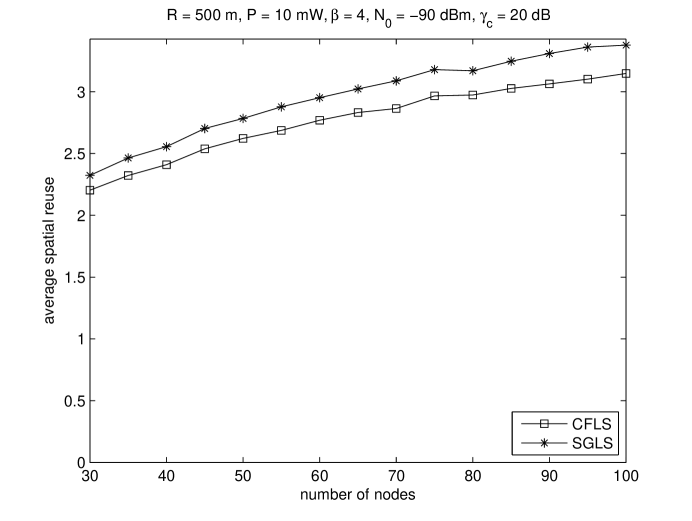
Figure 4.10: Spatial reuse vs. number of nodes for Experiment 1.

In the second experiment (Experiment 2), we assume that $R=700$ m, $P=15$ mW, $\beta=4$, $N_{0}=-85$ dBm and $\gamma_{c}=15$ dB. Thus, $R_{c}=110.7$ m. We vary the number of nodes from 70 to 150 in steps of 10. Figure 4.11 plots the average spatial reuse vs. number of nodes for both the algorithms.

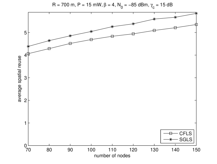
Figure 4.11: Spatial reuse vs. number of nodes for Experiment 2.

From the figures, we observe that SGLS achieves 5-10% higher spatial reuse than CFLS. However, this improvement in performance is obtained at the cost of higher computational complexity.

4.5 Discussion

In this chapter, we have proposed a novel point to point link scheduling algorithm based on an SINR graph representation of an STDMA wireless network under the physical interference model. Our results demonstrate that the spatial reuse for the proposed algorithm is higher than that of the ConflictFreeLinkSchedule algorithm. This is due to the fact that we have embedded interference conditions between pairs of nodes into the edge weights and normalized noise powers at receiver nodes into vertex weights of the SINR graph and consequently determined a conflict-free schedule. Our approach has the potential to scale with the number of nodes in the network.

Chapter 5 Point to Multipoint Link Scheduling: A Hybrid Approach

In this chapter, we investigate point to multipoint link scheduling in STDMA wireless networks. We generalize the definition of spatial reuse introduced in Chapter 2 for point to multipoint link scheduling. We propose a “hybrid” link scheduling algorithm based on a communication graph representation of the network and SINR conditions. We demonstrate that the proposed algorithm achieves higher spatial reuse than existing algorithms, without any increase in running time complexity.

The rest of this chapter is organized as follows. In Section 5.1, we describe our system model. We describe point to multipoint link scheduling based on the protocol interference model in Section 5.2 and describe its limitations in Section 5.3. In Section 5.4, we introduce spatial reuse as our performance metric and formulate the problem. In Section 5.5, we describe the proposed link scheduling algorithm. We evaluate its performance in Section 5.6 and derive its computational complexity in Section 5.7. We discuss the implications of our work in Section 5.8.

5.1 System Model

Our system model and notations are exactly as described in Section 2.1. However, we redefine and introduce terms that are applicable to point to multipoint link scheduling.

If node $k$ is within node $j$’s communication range, then $k$ is defined as a neighbor of $j$, since $k$ can decode $j$’s packet correctly (subject to Equation 2.6). Note that if node $k$ is outside node $j$’s communication range, then it can never decode $j$’s packet correctly (from Equation 2.6). The number of neighbors of node $j$ is denoted by $\eta(j)$.

A point to multipoint link schedule for an STDMA wireless network $\Phi(\cdot)$ is a mapping from the set of nodes to time slots. Let $C$ denote the number of time slots in a point to multipoint link schedule. For a given time slot $i$, $j^{th}$ point to multipoint transmission is denoted by $\{t_{i,j}\rightarrow\{r_{i,j,1},r_{i,j,2},\ldots,r_{i,j,\eta(t_{i,j})}\}\}$, where $t_{i,j}$ denotes the index of the node which transmits a packet and $r_{i,j,1},r_{i,j,2},\ldots,r_{i,j,\eta(t_{i,j})}$ denote the indices of neighboring nodes (neighbors of $t_{i,j}$) that receive the packet. Note that $r_{i,j,k}$ denotes $k^{th}$ receiver of $j^{th}$ transmission in time slot $i$. Let $M_{i}$ denote the number of concurrent point to multipoint transmissions in time slot $i$. A point to multipoint link schedule for an STDMA network $\Phi(\cdot)$ is denoted by $\Omega(\mathcal{B}_{1},\cdots,\mathcal{B}_{C})$, where

$${\mathcal{B}}_{i} := \{t_{i,1}\rightarrow\{r_{i,1,1},r_{i,1,2},\ldots,r_{i,1,\eta(t_{i,1})}\},\cdots,t_{i,M_{i}}\rightarrow\{r_{i,M_{i},1},r_{i,M_{i},2},\ldots,r_{i,M_{i},\eta(t_{i,M_{i}})}\}\}$$

$$= \mbox{set of concurrent point to multipoint transmissions in time slot $i$}.$$

Every point to multipoint schedule $\Omega(\cdot)$ must satisfy the following:

1. Operational constraints:

   1. A node cannot transmit and receive in the same time slot, i.e.,

      $$\{t_{i,j}\}\cap\{r_{i,k,1},\ldots,r_{i,k,\eta(t_{i,k})}\} = \phi\;\;\forall\;\;i=1,\ldots,C\;\;\forall\;\;j\neq k.$$ (5.1)

   2. A node cannot receive from multiple transmitters in the same time slot, i.e.,

      $$\{r_{i,j,1},\ldots,r_{i,j,\eta(t_{i,j})}\}\cap\{r_{i,k,1},\ldots,r_{i,k,\eta(t_{i,k})}\}=\phi\;\;\forall\;\;i=1,\ldots,C\;\;\forall\;\;j\neq k.$$ (5.2)

2. Range constraint: Every receiver is within the communication range of its intended transmitter, i.e.,

   $$D(t_{i,j},r_{i,j,k})\leqslant R_{c}\;\forall\;i=1,\ldots,C\;\forall\;j=1,\ldots,M_{i}\;\forall\;k=1,\ldots,\eta(t_{i,j}).$$ (5.3)

(a) An STDMA wireless network with six nodes.

(b) A point to multipoint link schedule for the network shown in Figure 5.1(a).

Figure 5.1: Example of STDMA network and point to multipoint link schedule.

For an example, consider the STDMA wireless network $\Phi(\cdot)$ shown in Figure 5.1(a). It consists of six nodes whose coordinates (in meters) are $1\equiv(-40,5)$, $2\equiv(0,0)$, $3\equiv(95,0)$, $4\equiv(135,0)$, $5\equiv(-75,0)$ and $6\equiv(0,-75)$. One of the possible point to multipoint link schedules for this STDMA network is shown in Figure 5.1(b). The schedule length is $C=5$ time slots and the schedule is defined by $\Omega(\mathcal{B}_{1},\mathcal{B}_{2},\mathcal{B}_{3},\mathcal{B}_{4},\mathcal{B}_{5})$, where

$$\mathcal{B}_{1} = \big{\{}t_{1,1}\rightarrow\{r_{1,1,1},r_{1,1,2},r_{1,1,3}\},\;t_{1,2}\rightarrow\{r_{1,2,1}\}\big{\}}$$

$$= \big{\{}1\rightarrow\{2,5,6\},\;4\rightarrow\{3\}\big{\}},$$

$$\mathcal{B}_{2} = \big{\{}t_{2,1}\rightarrow\{r_{2,1,1},r_{2,1,2}\}\big{\}}$$

$$= \big{\{}6\rightarrow\{1,2\}\big{\}},$$

$$\mathcal{B}_{3} = \big{\{}t_{3,1}\rightarrow\{r_{3,1,1},r_{3,1,2},r_{3,1,3},r_{3,1,4}\}\big{\}}$$

$$= \big{\{}2\rightarrow\{1,3,5,6\}\big{\}},$$

$$\mathcal{B}_{4} = \big{\{}t_{4,1}\rightarrow\{r_{4,1,1},r_{4,1,2}\}\big{\}}$$

$$= \big{\{}3\rightarrow\{2,4\}\big{\}},$$

$$\mathcal{B}_{5} = \big{\{}t_{5,1}\rightarrow\{r_{5,1,1},r_{5,1,2}\}\big{\}}$$

$$= \big{\{}5\rightarrow\{1,2\}\big{\}}.$$

After 5 time slots, the schedule repeats periodically, as shown in Figure 5.1(b).

A point to multipoint link scheduling algorithm is a set of rules that is used to determine a schedule $\Omega(\cdot)$. Typically, a scheduling algorithm is required to satisfy certain objectives.

Consider $k^{th}$ receiver of $j^{th}$ transmission in time slot $i$, i.e., receiver $r_{i,j,k}$. The power received at $r_{i,j,k}$ from its intended transmitter $t_{i,j}$ (signal power) is $\frac{P}{D^{\beta}(t_{i,j},r_{i,j,k})}$. The power received at $r_{i,j,k}$ from its unintended transmitters (interference power) is $\sum_{\stackrel{{\scriptstyle l=1}}{{l\neq j}}}^{M_{i}}\frac{P}{D^{\beta}(t_{i,l},r_{i,j,k})}$. Thus, the SINR at receiver $r_{i,j,k}$ is given by

$${\mbox{SINR}}_{r_{i,j,k}} = \frac{\frac{P}{D^{\beta}(t_{i,j},r_{i,j,k})}}{N_{0}+\sum_{\stackrel{{\scriptstyle l=1}}{{l\neq j}}}^{M_{i}}\frac{P}{D^{\beta}(t_{i,l},r_{i,j,k})}}.$$ (5.4)

According to the physical interference model [15], receiver $r_{i,j,k}$ can successfully decode the packet transmitted by $t_{i,j}$ if the SINR at $r_{i,j,k}$ is no less than the communication threshold $\gamma_{c}$, i.e.,

$${\mbox{SINR}}_{r_{i,j,k}} \geqslant \gamma_{c}.$$ (5.5)

A link schedule $\Omega(\cdot)$ is exhaustive if every two nodes $j$, $k$ who are neighbors of each other are included in the schedule exactly twice, once with $j$ being a transmitter and $k$ being one of its receivers, and during another time slot with $k$ being a transmitter and $j$ being one of its receivers.

5.2 Equivalence of Link Scheduling and Graph Vertex Coloring

In this section, we describe the equivalence between a point to multipoint link schedule for an STDMA wireless network and the coloring of vertices of the communication graph representation (see Section 2.2.1) of the network.

Parameter	Symbol	Value
transmission power	$P$	10 mW
path loss exponent	$\beta$	4
noise power spectral density	$N_{0}$	-90 dBm
communication threshold	$\gamma_{c}$	20 dB
interference threshold	$\gamma_{i}$	10 dB

Table 5.1: System parameters for STDMA networks shown in Figures 5.1(a) and 5.4.

Figure 5.2: Communication graph model of STDMA network described by Figure 5.1(a) and Table 5.1.

Consider the STDMA wireless network $\Phi(\cdot)$ whose deployment is shown in Figure 5.1(a). The system parameters for this network are given in Table 5.1. From (2.4), we obtain $R_{c}=100$ m. The corresponding communication graph representation $\mathcal{G}_{c}(\mathcal{V},\mathcal{E}_{c})$ is shown in Figure 5.2. The communication graph comprises of 6 vertices and 14 directed communication edges. The vertex and communication edge sets are given by

$$\mathcal{V} = \{v_{1},v_{2},v_{3},v_{4},v_{5},v_{6}\},$$ (5.6)

$$\mathcal{E}_{c} = \{v_{1}\stackrel{{\scriptstyle c}}{{\rightarrow}}v_{2},v_{2}\stackrel{{\scriptstyle c}}{{\rightarrow}}v_{1},v_{1}\stackrel{{\scriptstyle c}}{{\rightarrow}}v_{5},v_{5}\stackrel{{\scriptstyle c}}{{\rightarrow}}v_{1},v_{1}\stackrel{{\scriptstyle c}}{{\rightarrow}}v_{6},v_{6}\stackrel{{\scriptstyle c}}{{\rightarrow}}v_{1},v_{2}\stackrel{{\scriptstyle c}}{{\rightarrow}}v_{5},$$ (5.7)

$$v_{5}\stackrel{{\scriptstyle c}}{{\rightarrow}}v_{2},v_{2}\stackrel{{\scriptstyle c}}{{\rightarrow}}v_{6},v_{6}\stackrel{{\scriptstyle c}}{{\rightarrow}}v_{2},v_{2}\stackrel{{\scriptstyle c}}{{\rightarrow}}v_{3},v_{3}\stackrel{{\scriptstyle c}}{{\rightarrow}}v_{2},v_{3}\stackrel{{\scriptstyle c}}{{\rightarrow}}v_{4},v_{4}\stackrel{{\scriptstyle c}}{{\rightarrow}}v_{3}\}.$$

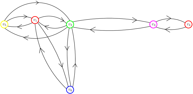
Figure 5.3: Vertex coloring of communication graph shown in Figure 5.2 corresponding to the link schedule shown in Figure 5.1(b).

Given the above representation of an STDMA network, a point to multipoint link schedule $\Omega(\cdot)$ can be considered as equivalent to assigning a unique color to every vertex in the communication graph, such that nodes with the same color transmit simultaneously in a particular time slot. For the example network considered, the link schedule shown in Figure 5.1(b) corresponds to the coloring of the vertices of the communication graph shown in Figure 5.3. Time slots 1, 2, 3, 4 and 5 in $\Omega(\cdot)$ correspond to colors red, blue, green, magenta and yellow in $\mathcal{V}$ respectively. Note that a coloring algorithm that uses the least number of colors also minimizes the schedule length.

Algorithms for assigning nodes to time slots (equivalently, colors) require that two vertices $v_{i}$, $v_{j}$ can be colored the same if and only if:

1. edge $v_{i}\stackrel{{\scriptstyle c}}{{\rightarrow}}v_{j}\not\in{\mathcal{E}}_{c}$ and edge $v_{j}\stackrel{{\scriptstyle c}}{{\rightarrow}}v_{i}\not\in{\mathcal{E}}_{c}$, i.e., there is no primary vertex conflict, and

2. there is no vertex $v_{k}$ such that $v_{i}\stackrel{{\scriptstyle c}}{{\rightarrow}}v_{k}\in{\mathcal{E}}_{c}$ and $v_{j}\stackrel{{\scriptstyle c}}{{\rightarrow}}v_{k}\in{\mathcal{E}}_{c}$ , i.e., there is no secondary vertex conflict.

These criteria are based on the operational constraints (5.1) and (5.2).

Algorithms based on the protocol interference model represent the network by a communication graph and utilize various graph coloring methodologies to devise heuristics which yield a minimum length schedule. Hence, such algorithms have the merit of low computational complexity. However, recent research suggests that these algorithms yield low network throughput. This aspect is elaborated in the following section.

5.3 Limitations of Algorithms based on Protocol Interference Model

In this section, we illustrate that algorithms based on the protocol interference model can result in schedules that yield low network throughput. Note that the limitations of point to multipoint link scheduling algorithm are similar to those of point to point link scheduling algorithms described in Section 2.3.

With the intent of maximizing the throughput of an STDMA network, algorithms based on the protocol interference model transform the scheduling problem to a vertex coloring problem for the communication graph representation of the network. For example, the BroadcastSchedule algorithm [16] works in two phases. In Phase 1, the vertices of the communication graph are labeled using the labeler function (Algorithm 2, Section 3.1). In Phase 2, vertices are considered in increasing order of label. For the vertex $u$ under consideration, it discards any color that leads to primary or secondary vertex conflicts with $u$. The least color among the residual set of non-conflicting colors is used to color vertex $u$. If no non-conflicting color exists, vertex $u$ is colored with a new color.

The simplification of the link scheduling problem in a wireless network as a vertex coloring problem on the communication graph can result in schedules that violate the SINR threshold condition (5.5). Specifically, algorithms based on the protocol interference model do not necessarily maximize the throughput of an STDMA network because:

1. They can result in high cumulative interference at a receiver, due to hard-thresholding based on communication radius. This is because the SINR at receiver $r_{i,j,k}$ decreases with an increase in the number of concurrent transmissions $M_{i}$, while $R_{c}$ has been defined for a single transmission only.

   

   Figure 5.4: An STDMA wireless network with six nodes.

   

   Figure 5.5: Communication graph model of STDMA network described by Figure 5.4 and Table 5.1.

   

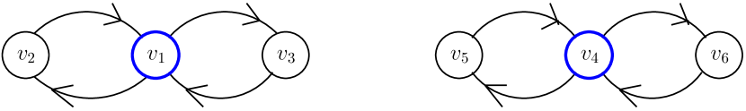
   Figure 5.6: Coloring of vertices $v_{1}$ and $v_{4}$ of graph shown in Figure 5.4.

   

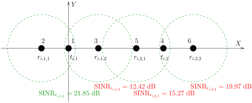
   Figure 5.7: Point to multipoint link scheduling algorithms based on protocol interference model can lead to high interference.

   For example, consider the STDMA wireless network whose deployment is shown in Figure 5.4. The network consists of six nodes whose coordinates (in meters) are $1\equiv(0,0)$, $2\equiv(-80,0)$, $3\equiv(90,0)$, $4\equiv(280,0)$, $5\equiv(200,0)$ and $6\equiv(370,0)$. The system parameters are shown in Table 5.1, which yields $R_{c}=100$ m. The communication graph model of the STDMA network is shown in Figure 5.5. Consider the transmission requests $1\rightarrow\{2,3\}$ and $4\rightarrow\{5,6\}$, which correspond to vertices $v_{1}$ and $v_{4}$ of the graph shown in Figure 5.5. Note that vertices $v_{1}$ and $v_{4}$ do not have primary or secondary vertex conflicts. So, to minimize the number of colors, such an algorithm will color these vertices with the same color, as shown in Figure 5.6. Equivalently, transmissions $1\rightarrow\{2,3\}$ and $4\rightarrow\{5,6\}$ will be scheduled in the same time slot, say time slot $i$. However, our computations show that the SINRs at receivers $r_{i,1,1}$, $r_{i,1,2}$, $r_{i,2,1}$ and $r_{i,2,2}$ are $21.85$ dB, $12.42$ dB, $15.27$ dB and $19.97$ dB respectively. Figure 5.7 shows the nodes of the network along with the labeled transmitter-receivers sets, receiver-centric communication zones and SINRs at the receivers. From the SINR threshold condition (5.5), transmission $t_{i,1}\rightarrow r_{i,1,1}$ is successful, while transmissions $t_{i,1}\rightarrow r_{i,1,2}$, $t_{i,2}\rightarrow r_{i,2,1}$ and $t_{i,2}\rightarrow r_{i,2,2}$ are unsuccessful. This leads to low network throughput.

2. Moreover, these algorithms are not aware of the topology of the network, i.e., they determine a link schedule without being cognizant of the exact positions of the transmitters and receivers.

As argued above, point to multipoint link scheduling algorithms based on the protocol interference model can result in low network throughput. In essence, algorithms that construct an approximate model of an STDMA network (communication graph) and concentrate on minimizing the schedule length do not necessarily maximize network throughput. This observation is developed into a proposal for an appropriate performance metric in Section 5.4.

5.4 Problem Formulation

In this section, we motivate the need for a performance metric that takes into account the SINR threshold condition (5.5) as the criterion for successful packet reception. Analogous to the notion of spatial reuse, we propose a performance metric for point to multipoint link scheduling, which is also termed as spatial reuse. We argue that spatial reuse is directly proportional to the number of successful point to multipoint transmissions. Finally, we formulate the scheduling problem from a perspective of maximizing spatial reuse.

Algorithms based on the protocol interference model are inadequate to design efficient point to multipoint link schedules. This is because these algorithms are entirely based on the communication graph $\mathcal{G}_{c}(\mathcal{V},\mathcal{E}_{c})$, which is a crude approximation of $\Phi(\cdot)$, and can lead to low network throughput, as argued in Section 5.3. On the other hand, from $\Phi(\cdot)$ and ${\mathcal{G}}_{c}(\cdot)$, one can exhaustively determine the link schedule $\Omega(\cdot)$ which yields highest network throughput according to the physical interference model. However, this is a combinatorial optimization problem of prohibitive complexity $(O(|\mathcal{V}|^{|\mathcal{V}|}))$ and is thus computationally infeasible.

To overcome these problems, we propose a point to multipoint link scheduling algorithm for STDMA wireless networks under the physical interference model. Our algorithm is based on the communication graph model ${\mathcal{G}}_{c}({\mathcal{V}},{\mathcal{E}}_{c})$ as well as SINR computations.

To evaluate the performance of our algorithm and compare it with existing link scheduling algorithms, we define the notion of spatial reuse. Consider the point to multipoint link schedule $\Omega(\cdot)$ for the STDMA network $\Phi(\cdot)$. Under the physical interference model, transmission $t_{i,j}\rightarrow r_{i,j,k}$ is successful if and only if (5.5) is satisfied. The spatial reuse of the link schedule $\Omega(\cdot)$ is defined as the average number of successful point to multipoint transmissions per time slot. Thus

$$\mbox{Spatial Reuse}\;=\;\varsigma := \frac{\sum_{i=1}^{C}\sum_{j=1}^{M_{i}}\frac{\sum_{k=1}^{\eta(t_{i,j})}I({\mbox{\scriptsize SINR}}_{r_{i,j,k}}\geqslant\gamma_{c})}{\eta(t_{i,j})}}{C},$$ (5.8)

where $I(A)$ denote the indicator function for event $A$, i.e., $I(A)=1$ if event $A$ occurs, $I(A)=0$ if event $A$ does not occur. Note that in (5.8), the number of nodes that successfully receive a transmitted packet is normalized by the number of neighbors of the transmitting node. A high value of spatial reuse corresponds to high network throughput.

The essence of STDMA is to have a reasonably large number of simultaneous and successful transmissions. For an STDMA wireless network which is operational for a long period of time, say $L$ time slots, the total number of successful point to multipoint transmissions is $L\varsigma$. Thus, a high value of spatial reuse directly translates to higher network throughput and the number of colors $C$ is relatively unimportant. Hence, spatial reuse turns out to be a crucial metric for the comparison of various STDMA link scheduling algorithms.

Our goal is to design a low complexity point to multipoint link scheduling algorithm that achieves high spatial reuse, where spatial reuse is given by (5.8). We only consider link schedules that are feasible and exhaustive.

5.5 MaxAverageSINRSchedule Algorithm

Our proposed point to multipoint link scheduling scheduling algorithm under the physical interference model is MaxAverageSINRSchedule (MASS), which considers the communication graph ${\mathcal{G}}_{c}({\mathcal{V}},{\mathcal{E}}_{c})$ and is described in Algorithm 7.

Algorithm 7 MaxAverageSINRSchedule (MASS)

1:  input: STDMA wireless network $\Phi(\cdot)$, communication graph $\mathcal{G}_{c}(\mathcal{V},\mathcal{E}_{c})$

2:  output: A coloring $C:{\mathcal{V}}\rightarrow\{1,2,\ldots\}$

3:  label the vertices of ${\mathcal{G}}_{c}$ randomly {Phase 1}

4:  for $j\leftarrow 1\mbox{ to }n$ do {Phase 2 begins}

5:     let $u$ be such that $L(u)=j$

6:     $C(u)\leftarrow\mbox{MaxAverageSINRColor}(u)$

7:  end for{Phase 2 ends}

In Phase 1, we label all the vertices randomly. Specifically, if $\mathcal{G}_{c}(\cdot)$ has $v$ vertices, we perform a random permutation of the sequence $(1,2,\ldots,v)$ and assign these labels to vertices with indices $1,2,\ldots,v$ respectively. Let $L(u)$ denote the label assigned to vertex $u$.

Algorithm 8 integer MaxAverageSINRColor($u$)

1:  input: STDMA wireless network $\Phi(\cdot)$, communication graph $\mathcal{G}_{c}(\mathcal{V},\mathcal{E}_{c})$

2:  output: A non-conflicting color

3:  ${\mathcal{C}}\leftarrow\mbox{set of existing colors}$

4:  ${\mathcal{C}}_{p}\leftarrow\{C(x):\mbox{$x$ is colored and is a neighbor of $u$}\}$

5:  ${\mathcal{C}}_{s}\leftarrow\{C(x):\mbox{$x$ is colored and is two hops away from $u$}\}$

6:  ${\mathcal{C}}_{nc}={\mathcal{C}}\setminus\{{\mathcal{C}}_{p}\cup{\mathcal{C}}_{s}\}$

7:  if ${\mathcal{C}}_{nc}\neq\phi$ then

8:     $r\leftarrow\mbox{color in ${\mathcal{C}}_{nc}$ which results in maximum average}$ SINR at neighbors of $u$

9:     if $\mbox{maximum average SINR}\geqslant\gamma_{c}$ then

10:        return $r$

11:     end if

12:  end if

13:  return $|\mathcal{C}|+1$

In Phase 2, the vertices are examined in increasing order of label and the MaxAverageSINRColor (MASC) function is used to assign a color to the vertex under consideration. The MASC function is explained in Algorithm 8. It begins by discarding all colors that have a primary or secondary vertex conflict with $u$, the vertex under consideration. Among the set of non-conflicting colors ${\mathcal{C}}_{nc}$, it chooses that color for $u$ which results in the maximum value of average SINR at the neighbors of $u$, provided this value exceeds the communication threshold. Intuitively, the average SINR is also a measure of the average distance of every neighbor of $u$ from all co-colored transmitters. The higher the average SINR, the higher is this average distance. We choose that color which results in the maximum average SINR at the neighbors of $u$, so that the additional interference at the neighbors of all co-colored transmitters is kept low. If no such color is found, it assigns a new color to $u$.

5.6 Performance Results

In this section, we describe our simulation model. We compare the performance of the proposed algorithm with existing point to multipoint link scheduling algorithms.

In our simulation experiments, the location of every node is generated randomly in a circular region of radius $R$. If $(X_{j},Y_{j})$ are the Cartesian coordinates of node $j$, then $X_{j}\sim U[-R,R]$ and $Y_{j}\sim U[-R,R]$ subject to $X_{j}^{2}+Y_{j}^{2}\leqslant R^{2}$. Equivalently, if $(R_{j},\Theta_{j})$ are the polar coordinates of node $j$, then $R_{j}^{2}\sim U[0,R^{2}]$ and $\Theta_{j}\sim U[0,2\pi]$. Using (2.4) and (2.5), we compute $R_{c}$ and $R_{i}$, and then map the STDMA network $\Phi(\cdot)$ to the communication graph $\mathcal{G}(\mathcal{V},\mathcal{E}_{c})$. Once the link schedule $\Omega(\cdot)$ is computed by every algorithm, the spatial reuse $\varsigma$ is computed using (5.8). We use two sets of prototypical values of system parameters in wireless networks [42]. For a given set of system parameters, we calculate the average spatial reuse by averaging $\varsigma$ over 1000 randomly generated networks. Keeping all other parameters fixed, we observe the effect of increasing the number of nodes on the average spatial reuse.

In our experiments, we compare the performance of the following algorithms:

1. BroadcastSchedule (BS) [16]

2. MaxAverageSINRSchedule (MASS)

In our first set of experiments (Experiment 1), we assume that $R=500$ m, $P=10$ mW, $\beta=4$, $N_{0}=-90$ dBm, $\gamma_{c}=20$ dB and $\gamma_{i}=10$ dB. Thus, $R_{c}=100$ m and $R_{i}=177.8$ m. We vary the number of nodes from 30 to 110 in steps of 5. Figure 5.8 plots the average spatial reuse vs. number of nodes for both the algorithms.

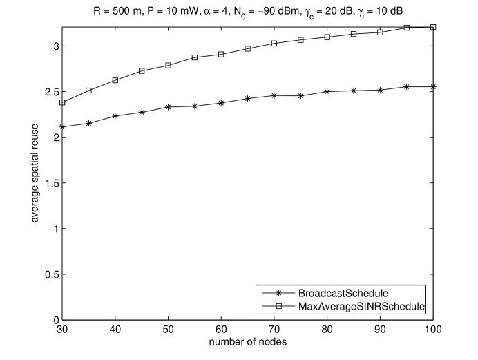
Figure 5.8: Average spatial reuse vs. number of nodes for Experiment 1.

In our second set of experiments (Experiment 2), we assume that $R=700$ m, $P=15$ mW, $\beta=4$, $N_{0}=-85$ dBm, $\gamma_{c}=15$ dB and $\gamma_{i}=7$ dB. Thus, $R_{c}=110.7$ m and $R_{i}=175.4$ m. We vary the number of nodes from 70 to 150 in steps of 5. Figure 5.9 plots the average spatial reuse vs. number of nodes for both the algorithms.

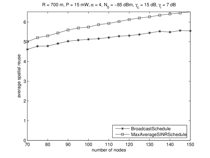
Figure 5.9: Average spatial reuse vs. number of nodes for Experiment 2.

From Figures 5.8 and 5.9, we observe that average spatial reuse increases with the number of nodes for both the algorithms. The MASS algorithm consistently yields higher average spatial reuse compared to BS. The spatial reuse of MASS is about $15\%$ higher than BS in Experiment 1 and $4\%$ higher in Experiment 2. This improvement in performance translates to substantially higher network throughput.

Also, an increase in the number of nodes in a given geographical area leads to an increase in the number of vertices having a primary or secondary vertex conflict with a given vertex. Hence, the number of non-conflicting colors for a given vertex also decreases. From this reduced set of non-conflicting colors, BroadcastSchedule chooses a color randomly, while MaxAverageSINRSchedule chooses a color based on SINR conditions. Since spatial reuse takes SINR threshold conditions into account, the gap between average spatial reuse values increases with number of nodes in Figures 5.8 and 5.9.

5.7 Analytical Result

In this section, we derive an upper bound on the running time (computational) complexity of the MaxAverageSINRSchedule algorithm. Let $v$ denote the number of vertices of the communication graph ${\mathcal{G}}_{c}({\mathcal{V}},{\mathcal{E}}_{c})$.

Theorem 5.7.1.

The running time of MaxAverageSINRSchedule is $O(v^{2})$.

Proof.

Assuming that an element can be chosen randomly and uniformly from a finite set in unit time ([53], Chapter 1), the running time of Phase 1 can be shown to be $O(v)$. In Phase 2, the vertex under consideration is assigned a color using MaxAverageSINRColor. The worst-case size of the set of colors to be examined $|{\mathcal{C}}_{nc}\cup{\mathcal{C}}_{p}\cup{\mathcal{C}}_{s}|$ is $O(v)$. With a careful implementation, MaxAverageSINRColor runs in time proportional to $|{\mathcal{C}}_{nc}|$, i.e., $O(v)$. Thus, the running time of Phase 2 is $O(v^{2})$. Finally, the overall running time of MaxAverageSINRSchedule is $O(v^{2})$. ∎

5.8 Discussion

In this chapter, we have developed a point to multipoint link scheduling algorithm for STDMA wireless networks under the physical interference model, namely MaxAverageSINRSchedule. The performance of our algorithm is superior to existing algorithms. A practical experimental modeling shows that, on an average, our algorithm achieves $15\%$ higher spatial reuse than the BroadcastSchedule algorithm [16]. Since link schedules are constructed offline only once and then used by the network for a long period of time, this improvement in performance directly translates to higher network throughput. The computational complexity of MaxAverageSINRSchedule is also comparable to the computational complexity of BroadcastSchedule. Therefore, MaxAverageSINRSchedule is a good candidate for efficient STDMA point to multipoint link scheduling algorithms.

Chapter 6 A Review of Random Access Algorithms for Wireless Networks

The MAC problem or multipoint to point problem is present in all communication networks, both wired and wireless. Multiple nodes (users) can access a single channel simultaneously to communicate with each other or a common receiver – the challenge is to design efficient channel access algorithms to achieve the desired performance in terms of throughput and delay. Several solutions to the MAC problem have been proposed depending on source traffic characteristics, channel models and Quality of Service (QoS) requirements of the users.

MAC protocols can be broadly classified into two types: fixed resource allocation protocols and random access protocols. Fixed resource allocation protocols such as Time Division Multiple Access (TDMA), Frequency Division Multiple Access (FDMA) and Code Division Multiple Access (CDMA) assign orthogonal or near-orthogonal channels to every user and are mostly implemented in voice-dominant wireless cellular networks. These protocols typically require the presence of a central entity (base station) to perform channel allocation and admission control, i.e., they are highly centralized. Though fixed resource allocation protocols are contention-free and can multiplex users with similar traffic characteristics easily, they suffer from low throughput and high channel access delay when the traffic is bursty and there are large number of users. On the other hand, in random access protocols, users vary their transmission probabilities or transmission times based on limited channel feedback, i.e., random access protocols are highly distributed. Random access protocols are more suitable for scenarios wherein many users with varied traffic requirements have to be multiplexed, i.e., the traffic is bursty.

Random access algorithms for satellite communications, multidrop telephone lines and multitap bus (“traditional random access algorithms”) have been well studied for the past four decades. These algorithms can be broadly classified into three categories: ALOHA [17], [59], Carrier Sense Multiple Access [60] and tree (or stack or splitting) algorithms [18]. Traditional random access algorithms have been implemented in practical systems. For example, ALOHA is used in most cellular networks to request channel access and also in satellite communication networks. Carrier Sense Multiple Access with Collision Detection (CSMA/CD) is used to resolve contentions in Local Area Networks (LANs).

On the other hand, random access algorithms that incorporate physical layer characteristics such as SINR and channel variations have only been studied recently. These algorithms, which have been primarily proposed for wireless networks, can be broadly classified into three categories: algorithms based on signal processing and diversity techniques, channel-aware ALOHA algorithms based on adapting the retransmission probabilities of contending users and “tree-like” algorithms based on adapting the set of contending users. Existing random access algorithms, such as Carrier Sense Multiple Access with Collision Avoidance (CSMA/CA ), are not channel-aware and can lead to low throughput. Thus, the design of physical layer aware random access algorithms can be a potential step towards achieving higher data rates in future wireless networks.

The organization of this chapter is as follows. Section 6.1 provides a summary of traditional random access algorithms along with the canonical system model, performance metrics and well-known random access techniques such as ALOHA and tree algorithms. This helps us understand channel-aware generalizations of these algorithms. In Section 6.2, we review research papers which employ signal processing and diversity techniques to correctly decode packets in random access wireless networks. We critically review some of the research which focus on channel-aware ALOHA and tree-like algorithms for wireless networks in Sections 6.3 and 6.4 respectively. Finally, we motivate the use of variable transmission power to increase the throughput of random access wireless networks in Section 6.5.

6.1 Traditional Random Access Algorithms

In this section, we describe the idealized slotted multiaccess model, which can be used to represent various multiaccess media such as satellite channels, multidrop telephone lines and multitap bus. We explain traditional random access algorithms such as ALOHA and tree algorithms. We also describe the performance metrics used to analyze and evaluate random access algorithms, namely, throughput, delay and stability.

Consider an idealized slotted multiaccess system with $m$ transmitting nodes and one receiver. The assumptions of the model are [22]:

1. Slotted system: All transmitted packets have the same length and each packet requires one time unit, called a slot, for transmission.

2. One of the following is usually assumed:

   1. Poisson arrivals: Packets arrive at each of the $m$ nodes according to an independent Poisson process. Let $\lambda$ be the overall arrival rate to the system and let $\frac{\lambda}{m}$ be the arrival rate at each transmitting node.

   2. Backlogged model: Every node always has a packet to transmit. Once a node transmits a packet successfully, a new packet is generated and awaits transmission.

3. Collision or perfect reception: If two or more nodes transmit a packet in a given slot, then there is a collision and the receiver obtains no information about the contents or the sources of transmitted packets. If only one node transmits a packet in a given slot, the packet is correctly received.

4. $\{0,1,e\}$ immediate feedback: At the end of each slot, every node obtains feedback from the receiver specifying whether 0 packet, 1 packet or more than one packet ($e$ denotes error) were transmitted in that slot.

5. Retransmission of collisions: Each packet involved in a collision must be retransmitted in some later slot, with further such retransmissions until the packet is successfully received. A node with a packet that must be retransmitted is said to be backlogged.

6. Only one of the following is assumed:

   1. No buffering: If one packet at a node is currently waiting for transmission or colliding with another packet during transmission, new arrivals at that node are discarded and never transmitted.

   2. Infinite set of nodes: The system has an infinite set of nodes and each new packet arrives at a new node.

For the analysis and performance evaluation of random access algorithms, the metrics of interest are:

1. Delay: Index packets as $1,2,3,\ldots$ according to their arrival instants. Let $D_{j}$ denote the delay experienced by $j^{th}$ packet. Then the average packet delay is defined as

   $$\mathcal{D} = \lim_{m\rightarrow\infty}E\left[\frac{1}{m}\sum_{j=1}^{m}D_{j}\right].$$ (6.1)

2. Throughput: The following are the two most common definitions of throughput:

   1. Throughput is the supremum of input packet arrival rates $\lambda$ such that the packet delay remains bounded, i.e.,

      $${\mathcal{T}}_{1} = \sup_{{\mathcal{D}}<\infty}\lambda.$$ (6.2)

   2. Let $n(t)$ denote the number of packets successfully transmitted in $[0,t]$. Define

      $$T(\lambda) = \left\{\begin{array}[]{ll}\lim_{t\rightarrow\infty}E\left[\frac{n(t)}{t}\right]&\mbox{if}\;\;{\mathcal{D}}<\infty,\\ 0&\mbox{otherwise}.\end{array}\right.$$

      Throughput is then defined as

      $$\mathcal{T}_{2} = \sup_{\lambda}T(\lambda).$$ (6.4)

3. Stability: A random access algorithm is stable if the throughput $\mathcal{T}>0$ and unstable if $\mathcal{T}=0$.

The research of random access algorithms began with the unslotted ALOHA (pure ALOHA) algorithm proposed by Abramson [17]. Each node, upon receiving a packet, transmits it immediately rather than waiting for a slot boundary. If a packet is involved in a collision, it is retransmitted after a random delay. It can be shown that unslotted ALOHA achieves a maximum throughput of $\frac{1}{2e}\approx 0.1839$ [22]. An advantage of unslotted ALOHA is that it can be used with variable-length packets.

Slotted ALOHA is a variation by Roberts [59] of the original unslotted ALOHA protocol proposed by Abramson. Each node simply transmits a newly arriving packet in the first slot after the packet arrival. When a collision occurs, every node sending a colliding packet discovers the collision at the end of the slot and becomes backlogged. Backlogged nodes wait for a random number of slots before retransmitting. The maximum throughput of slotted ALOHA can be shown to be $\frac{1}{e}\approx 0.3678$ [22]. Drift-analytic methods reveal that slotted ALOHA is unstable. To stabilize ALOHA, some techniques estimate $n$ or $p_{r}$, so as to maintain the attempt rate $G(n)$ at 1, resulting in a maximum stable throughput of $\frac{1}{e}$ [61], [62]. Unlike unslotted ALOHA, slotted ALOHA cannot be easily used with variable-sized packets. In slotted ALOHA, long packets must be broken up to fit into slots and short packets must be padded out to fill up slots.

Keeping the random access spirit of the ALOHA protocol, researchers attempted to design more efficient protocols. A highly successful approach consists of improving the control of the channel by carrier sensing, i.e., the Carrier Sense Multiple Access (CSMA) technique. In [22], the authors show that CSMA outperforms ALOHA. Research has shown that CSMA based protocols can achieve a throughput close to 0.9 [63]. The Ethernet protocol, which is used to connect computers on a wired LAN, utilizes Carrier Sense Multiple Access with Collision Detection (CSMA/CD).

In splitting algorithms, the set of colliding nodes splits into subsets, one of which transmits in the next slot. For a given colliding node, the choice of its subset depends on a pre-determined rule such as, the outcome of tossing an unbiased coin, a function of its arrival time or a function of its node identifier. If the collision is not resolved, a further splitting into subsets takes place. The algorithm proceeds recursively until all collisions are resolved.

Figure 6.1: Basic Tree Algorithm for three nodes $a$, $b$ and $c$.

Slot	Transmitting set	Waiting sets	Feedback
1	$U$	$\phi$	$e$
2	$L$	$R$	$e$
3	$LL$	$LR,R$	1
4	$LR$	$R$	$e$
5	$LRL$	$LRR,R$	0
6	$LRR$	$R$	$e$
7	$LRRL$	$LRRR,R$	1
8	$LRRR$	$R$	1
9	$R$	$\phi$	0

Table 6.1: Transmitting and waiting sets for basic tree algorithm shown in Figure 6.1.

Figure 6.2: Stack representation of transmitting and waiting nodes for basic tree algorithm shown in Figure 6.1.

In the Basic Tree Algorithm (BTA) [18], when a collision occurs, say in $k^{th}$ slot, all nodes not involved in the collision go into a waiting mode, and all those involved in the collision split into two subsets, according to the pre-determined rule. The first subset (“left” subset) transmits in slot $k+1$, and if that slot is idle or successful, the second subset (“right” subset) transmits in slot $k+2$. Alternatively, if another collision occurs in slot $k+1$, the first of the two subsets splits again, and the second subset waits for the resolution of that collision. Figure 6.1 exemplifies the operation of BTA for three nodes $a$, $b$ and $c$. Observe the binary tree structure of the sets of transmitting and waiting nodes in the figure. The transmitting and waiting sets in terms of subtrees of this binary tree are shown in Table 6.1, where $U=\{a,b,c\}$ denotes the set of all nodes that were involved in the initial collision. The labeling of the subtrees is recursive; for example, $LR$ denotes the right subtree of the left subtree of the original binary tree. The transmission order corresponds to that of a stack, as shown in Figure 6.2. In each slot, the stack is popped and all the nodes that were at the top of the stack transmit their packets. In case of a collision, the stack is pushed with nodes that join the right subset and then pushed again with nodes that join the left subset. In case of a success or idle, no push operations are performed on the stack. A Collision Resolution Period (CRP) is defined to be completed when a success or idle occurs and there are no remaining elements on the stack. In Figure 6.1, the length of the CRP is 9 slots.

During the operation of BTA, many new packets might arrive while a collision is being resolved. To solve this problem, at the end of a CRP, the set of nodes with new arrivals is immediately split into $j$ subsets, where $j$ is chosen so that the expected number of packets per subset is slightly greater than 1. The maximum throughput, optimized over the choice of $j$ as a function of expected number of waiting packets, is 0.43 packets per slot [18].

Figure 6.3: Modified Tree Algorithm for three nodes $a$, $b$ and $c$.

Slot	Transmitting set	Waiting sets	Feedback
1	$U$	$\phi$	$e$
2	$L$	$R$	$e$
3	$LL$	$LR,R$	1
4	$LR$	$R$	$e$
5	$LRL$	$LRR,R$	0
6	$LRRL$	$LRRR,R$	1
7	$LRRR$	$R$	1
8	$R$	$\phi$	0

Table 6.2: Transmitting and waiting sets for modified tree algorithm shown in Figure 6.3.

Figure 6.4: Stack representation of transmitting and waiting nodes for modified tree algorithm shown in Figure 6.3.

There exist variants of BTA that yield higher throughput. For example, in Modified Tree Algorithm (MTA), if a collision in slot $k$ is followed by an idle in slot $k+1$, then nodes which collided in slot $k$ refrain from transmitting in slot $k+2$. Instead, they further split into two subsets, one of which transmits in slot $k+2$. As an example, the operation of MTA for three nodes $a$, $b$ and $c$ is shown in Figure 6.3. Observe that the length of the CRP is 8 slots. For this example, the transmitting and waiting sets of subtrees are shown in Table 6.2, while the corresponding stack representation is shown in Figure 6.4. If an idle occurs in the current slot and a collision occurred in the previous slot (see Slot 5 in Figure 6.4), then the stack is popped a second time but the nodes at the top of the stack are not transmitted. Instead, these nodes split into right and left subsets and these subsets are pushed on the stack. This leads to fewer collisions and higher throughput compared to BTA. The maximum stable throughput of MTA is 0.46 packets per slot [64].

In First Come First Serve (FCFS) splitting algorithm [22], nodes involved in a collision split into two subsets based on the arrival times of collided packets. Using this approach, each subset consists of all packets that arrived in some given interval, and when a collision occurs, that interval will be split into two smaller intervals. By always transmitting packets that arrived in the earlier interval first, the algorithm transmits successful packets in the order of their arrival. The FCFS algorithm is stable for $\lambda<0.4871$ [22]. Conflict resolution protocols based on tree algorithms have provable stability properties [65].

We should point out that the random access algorithm proposed in Chapter 7 has a “tree structure” analogous to that of MTA. The detailed explanations of BTA and MTA provide a basic background to understand the dynamics of the proposed algorithm.

So far, we have summarized the methodology of traditional random access algorithms. In subsequent sections, we will focus on random access algorithms that are better suited for wireless networks such as WLANs and Wireless Metropolitan Area Networks (WMANs).

6.2 Signal Processing in Random Access

The collision model (Section 6.1, Assumption 4) is simple in that the onus of scheduling packets is left entirely to the MAC layer. On the contrary, physical layer techniques like multipacket reception, capture and network-assisted diversity are able to correctly decode packets from collisions by means such as coding and signal processing. These techniques are potential steps towards alleviating the burden of decoding packets from the MAC layer to the physical layer [66]. In this section, we review representative research work which exploits signal processing and diversity techniques to correctly decode the received packets in random access wireless networks.

With the advent of multiaccess techniques such as CDMA and Multiuser Detection [67], the first fundamental change in the collision model has been propounded in [68]. The authors offer the generalization that, in the presence of simultaneous transmissions, the reception can be described by conditional probabilities instead of deterministic failure. They propose the MultiPacket Reception (MPR) model defined by the matrix

$${\mathbf{C}} = \left[\begin{array}[]{cccc}C_{10}&C_{11}&&\\ C_{20}&C_{21}&C_{22}&\\ \vdots&&&\ddots\end{array}\right],$$ (6.8)

where $C_{ij}$ is the conditional probability that, given $i$ users transmit, $j$ out of $i$ transmissions are successful. Given $k$ users transmit at the same time, the average number of successfully received packets is given by

$$C_{k} = \sum_{j=0}^{k}jC_{kj}.$$ (6.9)

They show that ALOHA under MPR achieves stable throughput $\lim_{k\rightarrow\infty}C_{k}$ assuming that the limit exists. The stability and delay of finite-user slotted ALOHA with multipacket reception has been analyzed in [69].

In [70], the authors analyze the probability of capture in a multipoint to point wireless network. Analogous to the physical interference model, the capture model assumes that if a user’s SINR exceeds a threshold $\gamma$, then that user’s packet will be successfully received. They consider a realistic multiplicative propagation model in which the received power is obtained by multiplying the transmitted power by independent random variables representing fading, shadowing and path loss effects. To model the near-far effect, they assume that the distance $r$ of a mobile station from the base station is a random variable with distribution function $F_{R}(r)$. They show that, under broad conditions, the roll-off parameter $\delta$ of the distribution of power received from a mobile station is determined by the path loss exponent and $F_{R}(r)$. Additionally, $\delta$ is insensitive to other effects such as Rayleigh or Rician fading and log-normal shadowing. Finally, they show that in the limit of a large number of transmitters, the probability of capture is determined by the power capture threshold $\gamma$ and $\delta$. Though the analysis provided in [70] is mathematically robust, the authors do not describe any multiple access algorithm which achieves high throughput in wireless networks under the capture model, i.e., their result is more existential than constructive.

In [71], the authors propose Network-Assisted Diversity Multiple Access (NDMA), a technique for resolving collisions in wireless networks. They consider a wireless slotted random access network with Rayleigh fading and Additive White Gaussian Noise (AWGN). In NDMA, if $k$ users collide in a given slot, they repeat their transmissions $k-1$ times so that $k$ copies of the collided packets are received. Using signal separation principles, the receiver resolves a $k\times k$ source mixing problem to extract the signals of individual users, without incurring any penalty in throughput. The protocol has been extended to blind user detection [72] and has provable stability [73]. A good review of NDMA protocols is given in [74].

An alternative to employing signal processing techniques in random access wireless networks is to appropriately model the wireless channel and modify the well-researched ALOHA protocol. We review such research work in the next section.

6.3 Channel-Aware ALOHA Algorithms

In this section, we review representative research work whose central theme is to adapt the retransmission probabilities of users in random access wireless networks. In other words, we review research work which develops channel-aware ALOHA algorithms for wireless networks.

In [75], the authors develop a channel-aware ALOHA protocol for wireless networks. They assume a slotted system, block fading, $\{0,1,e\}$ feedback and a backlogged model (Section 6.1, Assumption 2b). They develop a distributed random access protocol in which each node only has knowledge of its own channel gain and nodes have long-term power constraints. A node transmits only if its channel gain exceeds $H_{0}$. For a system with $n$ nodes, the authors show that the optimum transmission probability is $\frac{\alpha(n)}{n}$, where $\alpha(n)\in(0,1]$ and $\alpha(n)\rightarrow 1$ as $n\rightarrow\infty$. Asymptotically, the ratio of the throughput of channel-aware ALOHA to the throughput of a centralized scheduler (which has knowledge of channel gains of all nodes) is shown to be $\frac{1}{e}$.

Opportunistic ALOHA algorithms for wireless networks have been studied in [76]. The authors consider a general reception model which encompasses $\{0,1,e\}$ feedback, capture as well as multipacket reception. Under the assumption that the Channel State Information (CSI) is known to each user, they propose a variant of slotted ALOHA, where the transmission probability is allowed to be a function of the CSI. The maximum throughput for the finite-user infinite-buffer model is derived. Finally, the theory is applied to CDMA networks with Linear Minimum Mean Square Error (LMMSE) receiver and matched filters.

The performance of slotted ALOHA in a wireless network with multiple destinations under the physical interference model is evaluated in [19]. A packet is successful only if it is captured at the receiver of its intended destination. The authors assume Poisson packet generation, $\{0,1,e\}$ feedback and circularly symmetric Gaussian distribution of users around each destination. They use a modified version of Rivest’s pseudo-Bayesian estimator [22] to estimate the backlog. Their simulation results demonstrate the effect of arrival rate, capture threshold, variance of user distribution and number of destinations on the throughput and energy efficiency per destination.

In [77], the author analyzes the throughput of slotted ALOHA in a multipoint to point wireless ad hoc network under the physical interference model. The cluster head employs reverse link power control, similar to IS-95 CDMA systems [78], to ensure that equal power is received from all nodes who attempt transmission in a time slot. The wireless channel is modeled as a multipacket reception channel. Assuming that one new packet arrives at each node in every time slot, the state of the system is characterized by a discrete time Markov chain with a steady state distribution. Finally, the author describes a technique to compute the network throughput.

In [79], the authors introduce spatial reuse slotted ALOHA, a random access protocol for random homogeneous mobile wireless networks. The occurrence of a collision is determined by the SINR at a receiver, i.e., the authors employ the physical interference model. They assume that nodes are randomly placed in a two-dimensional plane according to a Poisson point process and each node chooses a random destination at some finite distance. The powers at which stations can transmit are assumed to be independent and identically distributed (i.i.d.) and the wireless channel is characterized by its propagation path loss. Nodes move according to the random waypoint mobility model [80]. The authors characterize the interference process using tools from stochastic geometry. Subsequently, they determine the probability of channel access that maximizes the expected projected distance traversed per hop towards a destination, termed as “spatial density of progress”. Under the assumption that there is some non-degenerate node mobility, the authors show that the spatial density of progress is proportional to the square-root of the density of the nodes. Though the authors present a distributed ALOHA protocol and address certain implementation issues, their model does not represent real-world scenarios. Practical deployments of wireless nodes are better modeled by a uniform distribution in a finite plane rather than a Poisson point process in an infinite plane. Also, most of their results do not hold for static wireless networks (say, wireless mesh networks) since ergodicity assumptions no longer hold. Finally, their proposed routing protocol requires every node to have knowledge of locations and MAC states (receiver or transmitter) of all other nodes, which requires a lot of message passing between nodes (especially with mobile nodes) and is thus not scalable.

Instead of adapting the transmission probabilities of users in random access wireless networks, one can also adapt the transmission times of users based on the channel state and feedback from the receiver. Such techniques, which can be broadly termed as splitting algorithms or tree-like algorithms for wireless networks, are reviewed in the next section.

6.4 Splitting Algorithms

In this section, we review representative research work on random access algorithms whose main idea is to adapt the set of contending users based on feedback from the channel or the common receiver. In such work, the authors develop and analyze splitting (or tree or stack) algorithms for various models of the wireless channel and evaluate the performance of their algorithms via simulations.

In [81], the authors propose an opportunistic splitting algorithm for a multipoint to point wireless network. They assume a slotted system, block fading channel and $\{0,1,e\}$ feedback. Assuming that each user only knows its own channel gain and the number of backlogged users, the authors propose a distributed splitting algorithm to determine the user with the best channel gain over a sequence of mini-slots. The algorithm determines a lower threshold $H_{l}$ and a higher threshold $H_{h}$ for each mini-slot, such that only users whose channel gains lie between between $H_{l}$ and $H_{h}$ are allowed to transmit their packets. Based on results from “partitioning a sample with binary type questions” [82], they show that the average number of mini-slots required to determine the user with the best channel is 2.5, independent of the number of users and the fading distribution. However, their algorithm is impractical because it assumes that every user can accurately estimate the number of backlogged users.

In [83], the authors consider a random access network with infinite users, Poisson arrivals and $\{0,k,e\}$ immediate feedback, where $k$ is any positive integer. In contrast to standard tree algorithms (BTA, MTA, FCFS) that discard collided packets (Section 6.1, Assumption 4), they propose an algorithm that stores collided packets. The receiver extracts information from the collided packets by relying on successive interference cancellation techniques ([67], Chapter 7) and the tree structure of a collision resolution algorithm. Though their algorithm achieves a stable throughput of 0.693, it requires infinite storage and increased input voltage range at the receiver, which are not feasible in practical systems.

In [84], the author considers a multipoint to point wireless channel with and without capture and MPR. The channel provides Empty(E)/Non-Empty(NE) feedback to all active users and ‘success’ feedback to successful users only. The users do not need to know the starting times and ending times of collision resolution periods. For such a channel with E/NE binary feedback, the author proposes and analyzes a stack multiple access algorithm that is limited sensing and does not require any frame synchronization. The author considers two models for capture, namely Rayleigh fading with incoherent and coherent combining of joint interference power. For MPR, the author assumes a maximum of two successes during a collision. The maximum throughput of the algorithm is numerically evaluated be to 0.6548 when capture and MPR are present, and 0.2891 when both effects are absent. Though a novel splitting algorithm is proposed in [84], the author does not take into account throughput gains possible by varying transmission powers of users.

So far, we have reviewed research papers that either utilize signal processing techniques or adapt transmission probabilities or transmission times to increase the throughput in random access wireless networks. The throughput can be further increased by allowing users to use variable transmission powers. We review research papers which employ this idea in the next section.

6.5 Towards Power Controlled Random Access

In this section, we review representative research papers which focus on power control techniques in random access wireless networks. We then motivate the use of variable transmission power to increase the throughput in random access wireless networks.

In [85], the author considers a time-slotted CDMA-based wireless network wherein a finite number of nodes communicate with a common receiver. The author formulates the problem of determining the set of nodes that can transmit in each slot along with their corresponding transmission powers, subject to constraints on maximum transmission power and the SINRs of all transmissions exceeding the communication threshold. Due to its NP-hard nature, the problem is relaxed to a case wherein a node transmits with a certain probability in each slot. Equivalently, the problem of joint power control and link scheduling is transformed to a problem of power controlled random access, wherein the objective is to determine the probability of transmission $\Delta_{i}$ and transmission power $P_{i}$ for each node $i$, subject to constraints on maximum transmission power and the “expected SINR” exceeding the communication threshold. The author seeks to minimize a weighted sum of the maximum transmission power and maximum reciprocal probability, i.e., minimize $(\max_{i}P_{i}+\lambda\max_{i}\frac{1}{\Delta_{i}})$. This convex optimization problem is solved using techniques from geometric programming [86]. Finally, the author derives the probability of outage and delay distribution of buffered packets and demonstrates the efficacy of the schemes via simulations.

In [87], the authors investigate transmission power control and rate adaptation in random access wireless networks using game theoretic techniques. They consider multiple transmitters sharing a time-slotted channel to communicate equal-length packets with a common receiver. A user’s packet is successfully received if the SINR at the receiver is no less than the communication threshold, i.e., the authors employ the physical interference model. The random access problem is formulated as a game wherein each user selects its strategy (transmit or wait) at each stage of the game in a non-cooperative (independent) or cooperative manner. The authors evaluate equilibrium strategies for non-cooperative and cooperative symmetric random access games. Finally, the authors describe distributed power control and rate adaptation games for non-cooperative users for a collision channel with power-based capture. Their numerical results demonstrate improved expected user utilities when power control and rate adaptation are incorporated, at the expense of increased computational complexity. Though the authors propose a distributed random access algorithm based on game theoretic techniques, their algorithm is impractical because it assumes that every user knows $n$, the number of backlogged users, in each slot. However, in practice, $n$ can only be estimated using techniques such as Rivest’s pseudo-Bayesian algorithm [62].

Though researchers have addressed the problem of random access in wireless networks by considering various channel models, different types of feedback and realistic criteria for successful packet reception, only few of them exploit the idea that throughput gains are achievable in a random access wireless network by varying transmission powers of users. In general, varying the transmission powers of users leads to higher long-term average power. However, there exist wireless networks whose users do not have stringent energy requirements. For such scenarios, it would be useful to investigate the throughput gains achievable in the network by varying the transmission powers of users.

We envisage developing a power controlled random access algorithm for wireless networks under the physical interference model. We seek an algorithm that yields higher throughput than traditional random access algorithms. In cognizance of these requirements, we propose a power controlled splitting algorithm for wireless networks in Chapter 7. The algorithm is so designed that successful packets are transmitted in the order of their arrivals, i.e., in an FCFS manner.

In the system model considered in Chapter 7, if multiple transmissions occur, the receiver can decode a certain user’s packet correctly only if the received SINR exceeds a threshold, i.e., we consider a channel with power-based capture. The notion of capture has been addressed previously, though in different contexts [19], [84], [88]. However, in Chapter 7, we motivate the idea that a user can transmit at variable power levels to increase the chances of capture. Moreover, unlike [19], [84], [88], we assume $\{0,1,c,e\}$ feedback, where $0$, $1$ and $e$ denote idle, success and error respectively (Section 6.1, Assumption 4), and $c$ denotes capture in the presence of multiple transmissions. Note that the system model considered in Chapter 7 is different from those considered in existing works on splitting algorithms for wireless networks. For example, in [84], the author proposes a novel splitting algorithm, but does not take into account throughput gains possible by varying the transmission power. Though the authors of [81] propose a splitting algorithm to determine the user with the best channel gain, their algorithm is impractical because it assumes that every user can accurately estimate the number of backlogged users.

To the best of our knowledge, there is no existing work on variable power splitting algorithms for a wireless network under the physical interference model. The specification of the proposed algorithm along with its performance analysis and evaluation constitute the subject matter of the next chapter.

Chapter 7 Power Controlled FCFS Splitting Algorithm for Wireless Networks

In this chapter, we propound a random access algorithm that incorporates variable transmission powers in a multipoint to point wireless network. Specifically, we investigate random access in wireless networks under the physical interference model wherein the receiver is capable of power-based capture, i.e., a packet can be decoded correctly in the presence of multiple transmissions if the received SINR exceeds the communication threshold. We propose an interval splitting algorithm that varies the transmission powers of users based on channel feedback. We derive the maximum stable throughput of the proposed algorithm and demonstrate that it achieves better performance than the FCFS splitting algorithm [22] with uniform transmission power.

The rest of the chapter is organized as follows. We describe our system model in Section 7.1 and motivate variable control of transmission powers of contending users in Section 7.2. We describe the proposed random access algorithm and provide two illustrative examples in Section 7.3. We model the algorithm dynamics by a Markov chain and derive its maximum stable throughput in Section 7.4. The performance of the proposed algorithm is evaluated in Section 7.5. We conclude in Section 7.6.

7.1 System Model

Consider a multipoint to point wireless network. We assume the following:

1. Slotted system: Users (nodes) transmit fixed-length packets to a common receiver over a time-slotted channel. All users are synchronized such that the reception of a packet starts at an integer time and ends before the next integer time.

2. Poisson arrivals: The packet arrival process is Poisson distributed with overall rate $\lambda$, and each packet arrives to a new user that has never been assigned a packet before. After a user successfully transmits its packet, that user ceases to exist and does not contend for channel access in future time slots.

3. Channel model: The wireless channel is modeled by the path loss propagation model. The received signal power at a distance $D$ from the transmitter is given by $\frac{P}{D^{\beta}}$, where $P$ is the transmission power and $\beta$ is the path loss factor. We do not consider fading and shadowing effects.

4. Power-based capture: According to the physical interference model [15], a packet transmission from transmitter $t_{i,j}$ to receiver $r$ in $i^{th}$ time slot is successful if and only if the SINR at receiver $r$ is greater than or equal to the communication threshold $\gamma_{c}$, i.e.,

   $$\frac{\frac{P_{i,j}}{D^{\beta}(t_{i,j},r)}}{N_{0}+\sum_{\stackrel{{\scriptstyle k=1}}{{k\neq j}}}^{M_{i}}\frac{P_{i,k}}{D^{\beta}(t_{i,k},r)}}\geqslant\gamma_{c},$$ (7.1)

   where

   $$M_{i} = \mbox{number of concurrent transmitters in $i^{th}$ time slot},$$

   $$t_{i,j} = \mbox{$j^{th}$ transmitter in $i^{th}$ time slot}\;\;(j=1,2,\ldots,M_{i}),$$

   $$D(t_{i,j},r) = \mbox{Euclidean distance between $t_{i,j}$ and $r$},$$

   $$P_{i,j} = \mbox{transmission power of $t_{i,j}$},$$

   $$N_{0} = \mbox{thermal noise power spectral density}.$$

5. $\{0,1,c,e\}$ immediate feedback: By the end of each slot, users are informed of the feedback from the receiver immediately and without any error. The feedback is one of:

   1. idle $(0)$: when no packet transmission occurs,

   2. perfect reception $(1)$: when one packet transmission occurs and is received successfully,

   3. capture $(c)$: when multiple packet transmissions occur and only one packet is received successfully, or

   4. collision $(e)$: when multiple packet transmissions occur and no packet reception is successful.

   The receiver can distinguish between $1$ and $c$ by using energy detectors [83], [89]. Thus, by the end of every slot, only two bits are required to provide feedback from the receiver to all users. Note that two bits are required to provide feedback even for the classical $\{0,1,e\}$ feedback model. Thus, our $\{0,1,c,e\}$ immediate feedback assumption does not increase the number of bits required for feedback..

6. Gated Channel Access Algorithm (CAA): New packets are transmitted in the first available slot after previous conflicts are resolved. The time interval from the slot where an initial collision occurs up to and including the slot in which all users recognize that all packets involved in the collision have been successfully received, is called a Collision Resolution Period (CRP). Thus, new arrivals are inhibited from transmission during the CRP.

7. Equal distances: We assume that each user is at the same distance $D$ from the common receiver.

7.2 Motivation and Problem Formulation

The maximum stable throughput of the well-known FCFS splitting algorithm is 0.4871 [22], which is the highest throughput amongst a wide class of random access algorithms for wired networks. However, in a wireless network, transmission power of a node provides an extra degree of freedom, and higher throughputs are achievable.

Consider a scenario wherein all contending nodes transmit with equal power $P$ in a given time slot. When only one node transmits, its packet is successfully received if the SINR threshold condition (7.1) is satisfied, i.e.,

$$P\geqslant\gamma_{c}N_{0}D^{\beta}.$$ (7.2)

When $M$ nodes transmit concurrently with equal power $P$, where $M\geqslant 2$, the SINR corresponding to $i^{th}$ transmission is given by

$$\mbox{SINR}_{i} = \frac{\frac{P}{D^{\beta}}}{N_{0}+(M-1)\frac{P}{D^{\beta}}},$$ (7.3)

a quantity which is always less than 1. Since $\gamma_{c}>1$ for all practical narrowband communication receivers [70], $\mbox{SINR}_{i}<\gamma_{c}$ $\forall$ $i$ and all $M$ transmissions are unsuccessful. Thus, when multiple nodes transmit with equal power, a collision occurs irrespective of the transmission power $P$.

However, the above situation can be circumvented by varying transmission powers of users in some special cases. With relatively small attempt rates, when a collision occurs, it is most likely between only two packets [22]. In this case, if the receiver is capable of power-based capture, a collision between two nodes can be avoided by using different transmission powers. Specifically, one of the nodes, say $N_{1}$, transmits with minimum power $P_{1}$ such that, if it were the only node transmitting in that time slot, then its packet transmission will be successful. From (7.1), the required nominal power is

$$P_{1} = \gamma_{c}N_{0}D^{\beta}.$$ (7.4)

The other node, say $N_{2}$, transmits with minimum power $P_{2}$ such that if there is exactly one other node transmitting at nominal power $P_{1}$, then the packet transmitted by $N_{2}$ will be successful. From (7.1) and (7.4), we obtain

$$\frac{\frac{P_{2}}{D^{\beta}}}{N_{0}+\frac{P_{1}}{D^{\beta}}} = \gamma_{c},$$

$$P_{2} = \gamma_{c}(N_{0}D^{\beta}+P_{1}),$$

$$\therefore P_{2} = \gamma_{c}(1+\gamma_{c})N_{0}D^{\beta}.$$ (7.5)

Note that $\frac{P_{2}}{P_{1}}=1+\gamma_{c}$. We do not consider more than two power levels for the following reasons:

1. it complicates the power-control algorithm, and

2. most mobile wireless devices have constraints on peak transmission power.

Note that the above power control technique converts some collisions into “captures”. Thus, it has the potential of increasing the throughput of random access algorithms employing uniform transmission power.

We seek to design a distributed algorithm incorporating this power control technique, while still ensuring that the algorithm transmits successful packets in the order of their arrival, i.e., in an FCFS manner.

7.3 PCFCFS Interval Splitting Algorithm

In this section, we present an algorithmic description of the proposed Power Controlled First Come First Serve (PCFCFS) splitting algorithm. We also explain the behavior of the proposed algorithm by providing two illustrative examples.

7.3.1 Description

We first describe the notation. Slot $k$ is defined to be the time interval $[k,k+1)$. At each integer time $k$ ($k\geqslant 1$), the algorithm specifies the packets to be transmitted in slot $k$ to be the set of all packets that arrived in an earlier interval $[T(k),T(k)+\phi(k))$, which is defined as the allocation interval for slot $k$. The maximum size of the allocation interval is denoted by $\phi_{0}$, a parameter which will be optimized for maximum throughput in Section 7.4. Packets are indexed as $1,2,\ldots$ in the order of their arrival. Since the arrival times are Poisson distributed with rate $\lambda$, the inter-arrival times are exponentially distributed with mean $\frac{1}{\lambda}$. Let $a_{i}$ denote the arrival time of $i^{th}$ packet. Using the memoryless property of the exponential distribution (and without loss of generality), we assume that $a_{1}=0$. The transmission power of $i^{th}$ packet in slot $k$ is denoted by $P_{i}(k)$, where $P_{i}(k)\in\{0,P_{1},P_{2}\}$. Note that, if $P_{i}(k)=0$, then $i^{th}$ packet is not transmitted in slot $k$.

Algorithm 9 describes the proposed Power Controlled First Come First Serve (PCFCFS) splitting algorithm, which is the set of rules by which the users compute allocation interval parameters $\{T(k+1),\phi(k+1),\sigma(k+1)\}$ and transmission power $P_{i}(k+1)$ for slot $k+1$ in terms of the feedback and allocation interval parameters for slot $k$. In our algorithm, every allocation interval is tagged as a “left” $(\mathcal{L})$ or “right” $(\mathcal{R})$ interval. $\sigma(k)$ denotes the tag ($\mathcal{L}$ or $\mathcal{R}$) of allocation interval $[T(k),T(k)+\phi(k))$ in slot $k$. Moreover, whenever an allocation interval is split, it is always split into two equal-sized subintervals, and these subintervals $(\mathcal{L},\mathcal{R})$ are said to correspond to each other.

Algorithm 9 PCFCFS splitting algorithm

1:  input: $\phi_{0}$, $P_{1}$, $P_{2}$, arrivals $a_{1},a_{2},a_{3},\ldots$ in $[0,\tau)$ {Phase 1 begins}

2:  $T(1)\leftarrow 0$

3:  $\phi(1)\leftarrow\min(\phi_{0},1)$

4:  $\sigma(1)=\mathcal{R}$

5:  $\mbox{feedback}=0$ {Phase 1 ends}

6:  for $k\leftarrow 1\mbox{ to }\tau$ do {Phase 2 begins}

7:     if $\mbox{feedback}\neq c$ then {Phase 2a begins}

8:        for all $i$ such that $\scriptstyle T(k)\leqslant a_{i}<T(k)+\frac{\phi(k)}{2}$ do

9:           $P_{i}(k)=P_{2}$

10:        end for

11:        for all $i$ such that $\scriptstyle T(k)+\frac{\phi(k)}{2}\leqslant a_{i}<T(k)+\phi(k)$ do

12:           $P_{i}(k)=P_{1}$

13:        end for

14:     end if{Phase 2a ends}

15:     transmit packets whose arrivals times lie in $[T(k),T(k)+\phi(k))$ and obtain channel feedback {Phase 2b begins}

16:     if $\mbox{feedback}=e$ then

17:        $T(k+1)\leftarrow T(k)$

18:        $\phi(k+1)\leftarrow\frac{\phi(k)}{2}$

19:        $\sigma(k+1)\leftarrow\mathcal{L}$

20:     else if $\mbox{feedback}=c$ then

21:        $T(k+1)\leftarrow T(k)+\frac{\phi(k)}{2}$

22:        $\phi(k+1)\leftarrow\frac{\phi(k)}{2}$

23:        $\sigma(k+1)\leftarrow\mathcal{R}$

24:     else if $\mbox{feedback}=1$ and $\sigma(k)=\mathcal{L}$ then

25:        $T(k+1)\leftarrow T(k)+\phi(k)$

26:        $\phi(k+1)\leftarrow\phi(k)$

27:        $\sigma(k+1)\leftarrow\mathcal{R}$

28:     else if $\mbox{feedback}=0$ and $\sigma(k)=\mathcal{L}$ then

29:        $T(k+1)\leftarrow T(k)+\phi(k)$

30:        $\phi(k+1)\leftarrow\frac{\phi(k)}{2}$

31:        $\sigma(k+1)\leftarrow\mathcal{L}$

32:     else

33:        $T(k+1)\leftarrow T(k)+\phi(k)$

34:        $\phi(k+1)=\min(\phi_{0},k-T(k))$

35:        $\sigma(k+1)\leftarrow\mathcal{R}$

36:     end if{Phase 2b ends}

37:  end for{Phase 2 ends}

In Phase 1 of the algorithm, we initialize various quantities. $\tau$ denotes the number of slots for which the algorithm operates; ideally $\tau\rightarrow\infty$. By convention, the initial allocation interval is $[0,\min(\phi_{0},1))$, which is a right interval ($\mathcal{R}$). The initial channel feedback is assumed to be idle (0).

In Phase 2 of the algorithm, we determine power levels, obtain channel feedback and compute allocation interval parameters for each successive slot $k$. In Phase 2a, all users whose arrival times lie in the left half of the current allocation interval transmit with higher power $P_{2}$, while all users whose arrival times lie in the right half of the current allocation interval transmit with nominal power $P_{1}$. However, if a capture occurred in the previous slot $k-1$, all users in the current allocation interval transmit with nominal power $P_{1}$. Therefore, our algorithm always transmits successful packets in an FCFS manner. In Phase 2b, the allocation interval parameters are modulated based on the channel feedback. More specifically, if a collision occurs, then the left half of the current allocation interval becomes the new allocation interval. If a capture occurs, then the right half of the current allocation interval becomes the new allocation interval. If a success occurs and the current allocation interval is tagged as a left interval, then the corresponding right interval becomes the new allocation interval. If an idle occurs and the current allocation interval is tagged as a left interval, then the left half of the corresponding right interval becomes the new allocation interval. Otherwise, if a success or an idle occurs and the current allocation interval is tagged as a right interval, the waiting interval truncated to length $\phi_{0}$ becomes the new allocation interval, and a new Collision Resolution Period (CRP) begins in the next time slot $k+1$. Note that the transmit power levels in PCFCFS are variable and based on channel feedback, i.e., they are adaptive.

7.3.2 Examples

Figure 7.1: PCFCFS splitting algorithm illustrating a collision followed by an idle.

Figure 7.2: FCFS splitting algorithm illustrating a collision followed by an idle.

To illustrate the rules of the PCFCFS splitting algorithm for a single CRP, consider the example shown in Figure 7.1. In slot $k$, the allocation interval has no node in its left half and two nodes in its right half. Both these nodes transmit with nominal power $P_{1}$ and a collision occurs. So, the allocation interval is split, with the left interval $L$ being the allocation interval for slot $k+1$. An idle occurs in slot $k+1$. Next, the right subinterval $R$ is further split, with $RL$ being the allocation interval for slot $k+2$. The left node in $RL$ transmits with higher power $P_{2}$, while the right node in $RL$ transmits with nominal power $P_{1}$, resulting in a capture of the packet transmitted by the left node. The allocation interval is further split, with $RLR$ forming the allocation interval for slot $k+3$. Since a capture occurred in $RL$ in slot $k+2$, the corresponding right subinterval $RR$ is returned to the waiting interval in slot $k+3$. Post-capture, the lone node in $RLR$ transmits with nominal power $P_{1}$, resulting in a success and completing the CRP. For the same sequence of arrival times, the behavior of the FCFS algorithm with uniform transmission power $P$ is shown in Figure 7.2, where $\alpha(k)$ denotes the length of the allocation interval in slot $k$. Note that the FCFS algorithm requires 5 slots to resolve the collisions, while the proposed PCFCFS algorithm requires only 4 slots.

Figure 7.3: PCFCFS splitting algorithm illustrating a collision followed by another collision.

Figure 7.4: FCFS splitting algorithm illustrating a collision followed by another collision.

To further illustrate the rules of the PCFCFS splitting algorithm for a single CRP, consider the example shown in Figure 7.3. In slot $k$, the allocation interval has three nodes in its left half and one node in its right half. All ‘left half’ nodes transmit with higher power $P_{2}$, while the ‘right half’ node transmits with nominal power $P_{1}$, leading to a collision. So, the allocation interval is split, with the left interval $L$ being the allocation interval for slot $k+1$. In slot $k+1$, the allocation interval has one node in its left half, which transmits with higher power $P_{2}$, and two nodes in its right half, which transmit with nominal power $P_{1}$. Hence, a collision occurs, and the allocation interval $L$ is split into two equal sized subintervals $LL$ and $LR$, with $LL$ being the allocation interval for slot $k+2$. Since a collision is followed by another collision, the right interval $R$ is returned to the waiting interval in slot $k+2$. In slot $k+2$, there is only one node in the allocation interval. Since this lone node lies in the right half of the allocation interval, it transmits with nominal power $P_{1}$, leading to a success. Thus, $LR$ becomes the allocation interval for slot $k+3$. For this allocation interval, the node in the left half transmits with higher power $P_{2}$ and the node in the right half transmits with nominal power $P_{1}$, resulting in a capture of the packet transmitted by the former node. Consequently, $LRR$ becomes the new allocation interval for slot $k+4$. Finally, in slot $k+4$, the lone node transmits with nominal power $P_{1}$, leading to a deterministic success and completing the CRP. For the same sequence of arrival times, the behavior of the FCFS algorithm with uniform transmission power $P$ is shown in Figure 7.4. Note that the FCFS algorithm requires 6 slots to resolve the collisions, while the proposed PCFCFS algorithm requires only 5 slots.

7.4 Throughput Analysis

Figure 7.5: Discrete Time Markov Chain representing a CRP of PCFCFS splitting algorithm.

The evolution of a CRP can be represented by the Discrete Time Markov Chain (DTMC) shown in Figure 7.5. Every state in the DTMC is a pair $(\sigma,i)$, where $\sigma$ is the status $\{L,L^{\prime},R,R^{\prime},C\}$ and $i$ is the number of times the original allocation interval (of length $\phi_{0}$) has been split. State $(R,0)$ corresponds to the initial slot of a CRP. If an idle or a success occurs, the CRP ends immediately and a new CRP begins in the next slot. If a capture occurs, a transition occurs to state $(C,1)$, where $C$ indicates that capture has occurred in the allocation interval. If a collision occurs in $(R,0)$, a transition occurs to state $(L,1)$. Each subsequent idle in a left allocation interval generates one additional split with a smaller left allocation interval, corresponding to a transition to $(L^{\prime},i+1)$, where $L^{\prime}$ indicates that the current left allocation interval has been reached after a collision (in some time slot) followed by one or more idles. A collision in an allocation interval generates one additional split with a smaller left allocation interval, corresponding to a transition to $(L,i+1)$, where $L$ indicates that the current left allocation interval has been reached just after a collision. A capture in an allocation interval generates an additional split with a smaller right allocation interval and corresponds to a transition to $(C,i+1)$. This is followed by a success from $(C,i+1)$ to $(R,0)$, thus ending the CRP. A success in a left allocation interval leads to the corresponding right allocation interval with no additional split, which causes a transition from $(L,i)$ to $(R,i)$, or $(L^{\prime},i)$ to $(R^{\prime},i)$. A success in $(R^{\prime},i)$ causes a transition to $(R,0)$, thus ending the CRP. It can be easily verified that the states and transitions in Figure 7.5 constitute a Markov chain, i.e., each transition from every state is independent of the path used to reach the given state.

We now analyze a single CRP. Assume that the size of the initial allocation interval is $\phi_{0}$ (corresponding to state $(R,0)$). Each splitting of the allocation interval halves this, so that states $(L,i)$, $(L^{\prime},i)$, $(R,i)$, $(R^{\prime},i)$ and $(C,i)$ in Figure 7.5 correspond to allocation intervals of size $2^{-i}\phi_{0}$. Since the arrival process is Poisson with rate $\lambda$, the number of packets in the original allocation interval is a Poisson random variable (r.v.) with mean $\lambda\phi_{0}$. Consequently, the a priori distributions on the number of packets in disjoint subintervals are independent and Poisson. Define $G_{i}$ as the expected number of packets in an interval that has been split $i$ times. Thus

$$G_{i} = 2^{-i}\lambda\phi_{0}\;=\;2^{-i}G_{0}\;\;\;\forall\;\;\;i\geqslant 0,$$ (7.6)

$$\therefore G_{i} = \frac{1}{2}G_{i-1}\;\;\;\forall\;\;\;i\geqslant 1.$$ (7.7)

We view $(R,0)$ as the starting state as well as the final state. For brevity in notation, the transition probability from state $(A,i)$ to state $(B,j)$ is denoted by $P_{A_{i},B_{j}}$, where $A,B\in\{L,L^{\prime},R,R^{\prime},C\}$ and $i,j\in\{0\}\cup{\mathbb{Z}}^{+}$ (see Figure 7.5). For example, the transition probability from $(L,1)$ to $(C,2)$ is denoted by $P_{L_{1},C_{2}}$.

Figure 7.6: Notation for number of packets in left and right subintervals of the original allocation interval.

$P_{R_{0},R_{0}}$ is the probability of an idle or success in the first slot of the CRP. Since the number of packets in the initial allocation interval is Poisson with mean $G_{0}$, the probability of 0 or 1 packet is

$$P_{R_{0},R_{0}} = (1+G_{0})e^{-G_{0}}.$$ (7.8)

$P_{R_{0},C_{1}}$ is the probability of capture in the first slot of a CRP. Let $x_{L}$ and $x_{R}$ denote the number of packets in the left and right halves of the original allocation interval respectively, as shown in Figure 7.6. Capture occurs if and only if $x_{L}=1$ and $x_{R}=1$. $x_{L}$ and $x_{R}$ are independent Poisson r.v.s of mean $G_{1}$ each. Thus

$$P_{R_{0},C_{1}} = \Pr(x_{L}=1,x_{R}=1),$$

$$= \Pr(x_{L}=1)\Pr(x_{R}=1),$$

$$= G_{1}^{2}e^{-2G_{1}},$$

$$\therefore P_{R_{0},C_{1}} = \frac{G_{0}^{2}}{4}e^{-G_{0}}.$$ (7.9)

State $(L,1)$ is entered after collision in state $(R,0)$. Using (7.8) and (7.9), this occurs with probability

$$P_{R_{0},L_{1}} = 1-P_{R_{0},R_{0}}-P_{R_{0},C_{1}},$$

$$\therefore P_{R_{0},L_{1}} = 1-\Big{(}1+G_{0}+\frac{G_{0}^{2}}{4}\Big{)}e^{-G_{0}}.$$ (7.10)

Since a capture is always followed by a deterministic success,

$$P_{C_{i},R_{0}} = 1\;\;\forall\;\;i\geqslant 1.$$ (7.11)

Lemma 7.4.1.

The outgoing transition probabilities from $(L,i)$, where $i\geqslant 1$, are given by

$$P_{L_{i},R_{i}} = \frac{(1-e^{-G_{i}}-G_{i}e^{-G_{i}})G_{i}e^{-G_{i}}}{1-\Big{(}1+G_{i-1}+\frac{G_{i-1}^{2}}{4}\Big{)}e^{-G_{i-1}}},$$ (7.12)

$$P_{L_{i},L_{i+1}^{\prime}} = \frac{(1-e^{-G_{i}}-G_{i}e^{-G_{i}})e^{-G_{i}}}{1-\Big{(}1+G_{i-1}+\frac{G_{i-1}^{2}}{4}\Big{)}e^{-G_{i-1}}},$$ (7.13)

$$P_{L_{i},C_{i+1}} = \frac{\frac{G_{i}^{2}}{4}e^{-G_{i}}}{1-\Big{(}1+G_{i-1}+\frac{G_{i-1}^{2}}{4}\Big{)}e^{-G_{i-1}}},$$ (7.14)

$$P_{L_{i},L_{i+1}} = \frac{1-(1+G_{i}+\frac{G_{i}^{2}}{4})e^{-G_{i}}}{1-\Big{(}1+G_{i-1}+\frac{G_{i-1}^{2}}{4}\Big{)}e^{-G_{i-1}}}.$$ (7.15)

Proof.

Refer to Figure 7.5. For $i=1$, $(L,i)$ is entered only via a collision in $(R,i-1)$. For $i=2$, $(L,i)$ is entered only via a collision in $(L,i-1)$ or $(R,i-1)$. For $i\geqslant 3$, $(L,i)$ is entered only via a collision in $(L^{\prime},i-1)$, $(L,i-1)$, $(R,i-1)$ or $(R^{\prime},i-1)$. In every case, a subinterval $Y$ is split into $YL$ and $YR$, and $YL$ becomes the new allocation interval. Let $x_{YL}$ and $x_{YR}$ denote the number of packets in $YL$ and $YR$ respectively. A priori, $x_{YL}$ and $x_{YR}$ are independent Poisson r.v.s of mean $G_{i}$ each. The event that a collision occurred in the previous state is $\{x_{YL}+x_{YR}\geqslant 2\}\cap\{x_{YL}=x_{YR}=1\}^{c}=:\mathcal{C}_{Y}$. Note that $x_{YL}+x_{YR}=x_{Y}$ is a Poisson r.v. of mean $G_{i-1}$. From (7.7), $G_{i}=\frac{1}{2}G_{i-1}$ $\forall$ $i\geqslant 1$. The probability of success in $(L,i)$ is the probability that $x_{YL}=1$ conditional on $\mathcal{C}_{Y}$, i.e.,

$$P_{L_{i},R_{i}} = \Pr(x_{YL}=1|\mathcal{C}_{Y}),$$

$$= \frac{\Pr(\mathcal{C}_{Y}|x_{YL}=1)\Pr(x_{YL}=1)}{\Pr(\mathcal{C}_{Y})},$$

$$= \frac{\Pr(\{x_{YR}=1\}\cap\{x_{YR}=1\}^{c})\Pr(x_{YL}=1)}{\Pr(\mathcal{C}_{Y})},$$

$$= \frac{\Pr(x_{YR}\geqslant 2)\Pr(x_{YL}=1)}{\Pr(\{x_{YL}+x_{YR}\geqslant 2\}\cap\{x_{YL}=x_{YR}=1\}^{c})},$$

$$= \frac{\Pr(x_{YR}\geqslant 2)\Pr(x_{YL}=1)}{\Pr(x_{Y}\geqslant 2)-\Pr(x_{YL}=1)\Pr(x_{YR}=1)},$$

$$= \frac{(1-e^{-G_{i}}-G_{i}e^{-G_{i}})G_{i}e^{-G_{i}}}{1-e^{-G_{i-1}}-G_{i-1}e^{-G_{i-1}}-G_{i}^{2}e^{-2G_{i}}},$$

$$\therefore P_{L_{i},R_{i}} = \frac{(1-e^{-G_{i}}-G_{i}e^{-G_{i}})G_{i}e^{-G_{i}}}{1-\Big{(}1+G_{i-1}+\frac{G_{i-1}^{2}}{4}\Big{)}e^{-G_{i-1}}}.$$ (7.16)

The probability of idle in $(L,i)$ is the probability that $x_{YL}=0$ conditional on $\mathcal{C}_{Y}$, i.e.,

$$P_{L_{i},L_{i+1}^{\prime}} = \Pr(x_{YL}=0|\mathcal{C}_{Y}),$$

$$= \frac{\Pr(\mathcal{C}_{Y}|x_{YL}=0)\Pr(x_{YL}=0)}{\Pr(\mathcal{C}_{Y})},$$

$$= \frac{\Pr(\{x_{YR}\geqslant 2\}\cap\{x_{YR}=1\}^{c})\Pr(x_{YL}=0)}{\Pr(\mathcal{C}_{Y})},$$

$$= \frac{\Pr(x_{YR}\geqslant 2)\Pr(x_{YL}=0)}{\Pr(\{x_{YL}+x_{YR}\geqslant 2\}\cap\{x_{YL}=x_{YR}=1\}^{c})},$$

$$= \frac{\Pr(x_{YR}\geqslant 2)\Pr(x_{YL}=0)}{\Pr(x_{Y}\geqslant 2)-\Pr(x_{YL}=1)\Pr(x_{YR}=1)},$$

$$= \frac{(1-e^{-G_{i}}-G_{i}e^{-G_{i}})e^{-G_{i}}}{1-e^{-G_{i-1}}-G_{i-1}e^{-G_{i-1}}-G_{i}^{2}e^{-2G_{i}}},$$

$$\therefore P_{L_{i},L_{i+1}^{\prime}} = \frac{(1-e^{-G_{i}}-G_{i}e^{-G_{i}})e^{-G_{i}}}{1-\Big{(}1+G_{i-1}+\frac{G_{i-1}^{2}}{4}\Big{)}e^{-G_{i-1}}}.$$ (7.17)

Let $x_{YLL}$ and $x_{YLR}$ denote the number of packets in $YLL$ and $YLR$ respectively. $x_{YLL}$ and $x_{YLR}$ are independent Poisson r.v.s of mean $G_{i+1}$ each, and $x_{YLL}+x_{YLR}=x_{YL}$. The probability of capture in $(L,i)$ is the probability that $x_{YLL}=1$ and $x_{YLR}=1$ conditional on $\mathcal{C}_{Y}$, i.e.,

$$P_{L_{i},C_{i+1}} = \Pr(x_{YLL}=1,x_{YLR}=1|\mathcal{C}_{Y}),$$

$$= \frac{\Pr(\mathcal{C}_{Y}|x_{YLL}=1,x_{YLR}=1)\Pr(x_{YLL}=1,x_{YLR}=1)}{\Pr(\{x_{YL}+x_{YR}\geqslant 2\}\cap\{x_{YL}=x_{YR}=1\}^{c})},$$

$$= \frac{\Pr(\mathcal{C}_{Y}|x_{YL}=2)\Pr(x_{YLL}=1)\Pr(x_{YLR}=1)}{\Pr(\{x_{YL}+x_{YR}\geqslant 2\}\cap\{x_{YL}=x_{YR}=1\}^{c})},$$

$$= \frac{\Pr(x_{YR}\geqslant 0)\Pr(x_{YLL}=1)\Pr(x_{YLR}=1)}{\Pr(x_{Y}\geqslant 2)-\Pr(x_{YL}=1)\Pr(x_{YR}=1)},$$

$$= \frac{1.G_{i+1}^{2}e^{-2G_{i+1}}}{1-e^{-G_{i-1}}-G_{i-1}e^{-G_{i-1}}-G_{i}^{2}e^{-2G_{i}}},$$

$$\therefore P_{L_{i},C_{i+1}} = \frac{\frac{G_{i}^{2}}{4}e^{-G_{i}}}{1-\Big{(}1+G_{i-1}+\frac{G_{i-1}^{2}}{4}\Big{)}e^{-G_{i-1}}}.$$ (7.18)

From (7.16), (7.17) and (7.18), we obtain

$$P_{L_{i},L_{i+1}} = 1-P_{L_{i},R_{i}}-P_{L_{i},L_{i+1}^{\prime}}-P_{L_{i},C_{i+1}},$$

$$\therefore P_{L_{i},L_{i+1}} = \frac{1-\Big{(}1+G_{i}+\frac{G_{i}^{2}}{4}\Big{)}e^{-G_{i}}}{1-\Big{(}1+G_{i-1}+\frac{G_{i-1}^{2}}{4}\Big{)}e^{-G_{i-1}}}.$$ (7.19)

∎

Lemma 7.4.2.

The outgoing transition probabilities from $(R,i)$ are given by

$$P_{R_{i},C_{i+1}} = \frac{\frac{G_{i}^{2}}{4}e^{-G_{i}}}{1-(1+G_{i})e^{-G_{i}}}\;\;\forall\;\;i\geqslant 1,$$ (7.20)

$$P_{R_{i},L_{i+1}} = \frac{1-\big{(}1+G_{i}+\frac{G_{i}^{2}}{4}\big{)}e^{-G_{i}}}{1-(1+G_{i})e^{-G_{i}}}\;\;\forall\;\;i\geqslant 1.$$ (7.21)

Proof.

Refer to Figure 7.5. For $i\geqslant 1$, $(R,i)$ is entered only via a success in $(L,i)$. Recall that $(L,i)$ was entered only via a collision from a previous state. We use the notation introduced in the proof of Lemma 7.4.1. Define the event

$$\mathcal{S}_{YL} := \mathcal{C}_{Y}\cap\{x_{YL}=1\},$$

$$= \{x_{YL}+x_{YR}\geqslant 2\}\cap\{x_{YL}=x_{YR}=1\}^{c}\cap\{x_{YL}=1\},$$

$$= \{x_{YR}\geqslant 1\}\cap\{x_{YR}=1\}^{c}\cap\{x_{YL}=1\},$$

$$\therefore\mathcal{S}_{YL} = \{x_{YR}\geqslant 2\}\cap\{x_{YL}=1\}.$$ (7.22)

Let $x_{YRL}$ and $x_{YRR}$ denote the number of packets in $YRL$ and $YRR$ respectively. $x_{YRL}$ and $x_{YRR}$ are independent Poisson r.v.s of mean $G_{i+1}$ each. Since $x_{YR}\geqslant 2$, a success or an idle can never occur in state $(R,i)$. Note that $x_{YR}=x_{YRL}+x_{YRR}$. The probability of capture in state $(R,i)$ is the probability that $x_{YRL}=1$ and $x_{YRR}=1$ conditional on $\mathcal{S}_{YL}$, i.e.,

$$P_{R_{i},C_{i+1}} = \Pr(x_{YRL}=1,x_{YRR}=1|x_{YR}\geqslant 2,x_{YL}=1),$$

$$= \Pr(x_{YRL}=1,x_{YRR}=1|x_{YR}\geqslant 2),$$

$$= \frac{\Pr(x_{YR}\geqslant 2|x_{YRL}=1,x_{YRR}=1)\Pr(x_{YRL}=1,x_{YRR}=1)}{\Pr(x_{YR}\geqslant 2)},$$

$$= \frac{\Pr(x_{YRL}+x_{YRR}\geqslant 2|x_{YRL}=1,x_{YRR}=1)\Pr(x_{YRL}=1,x_{YRR}=1)}{\Pr(x_{YR}\geqslant 2)},$$

$$= \frac{1.\Pr(x_{YRL}=1)\Pr(x_{YRR}=1)}{\Pr(x_{YR}\geqslant 2)},$$

$$= \frac{G_{i+1}^{2}e^{-2G_{i+1}}}{1-e^{-G_{i}}-G_{i}e^{-G_{i}}},$$

$$\therefore P_{R_{i},C_{i+1}} = \frac{\frac{G_{i}^{2}}{4}e^{-G_{i}}}{1-(1+G_{i})e^{-G_{i}}}.$$ (7.23)

From (7.23), we obtain

$$P_{R_{i},L_{i+1}} = 1-P_{R_{i},C_{i+1}},$$

$$= 1-\frac{\frac{G_{i}^{2}}{4}e^{-G_{i}}}{1-(1+G_{i})e^{-G_{i}}},$$

$$\therefore P_{R_{i},L_{i+1}} = \frac{1-\big{(}1+G_{i}+\frac{G_{i}^{2}}{4}\big{)}e^{-G_{i}}}{1-(1+G_{i})e^{-G_{i}}}.$$ (7.24)

∎

Lemma 7.4.3.

The outgoing transition probabilities from $(L^{\prime},i)$ are given by

$$P_{L_{i}^{\prime},R_{i}^{\prime}} = \frac{(1-e^{-G_{i}})G_{i}e^{-G_{i}}}{1-(1+G_{i-1})e^{-G_{i-1}}}\;\;\forall\;\;i\geqslant 2,$$ (7.25)

$$P_{L_{i}^{\prime},L_{i+1}^{\prime}} = \frac{(1-e^{-G_{i}}-G_{i}e^{-G_{i}})e^{-G_{i}}}{1-(1+G_{i-1})e^{-G_{i-1}}}\;\;\forall\;\;i\geqslant 2,$$ (7.26)

$$P_{L_{i}^{\prime},C_{i+1}} = \frac{\frac{G_{i}^{2}}{4}e^{-G_{i}}}{1-(1+G_{i-1})e^{-G_{i-1}}}\;\;\forall\;\;i\geqslant 2,$$ (7.27)

$$P_{L_{i}^{\prime},L_{i+1}} = \frac{1-\big{(}1+G_{i}+\frac{G_{i}^{2}}{4}\big{)}e^{-G_{i}}}{1-(1+G_{i-1})e^{-G_{i-1}}}\;\;\forall\;\;i\geqslant 2.$$ (7.28)

Proof.

Refer to Figure 7.5. For $i=2$, $(L^{\prime},i)$ is entered only by an idle in $(L,i-1)$. For $i\geqslant 3$, state $(L^{\prime},i)$ is entered by an idle in $(L^{\prime},i-1)$ or an idle in $(L,i-1)$. In every case, a residual right subinterval, say $Z$, is split into $ZL$ and $ZR$, and $ZL$ becomes the new allocation interval. Note that $(L^{\prime},i)$ can be entered if and only if there is a collision (in some time slot) followed by one or more idles. Therefore, $Z$ must contain at least two packets. Let $x_{ZL}$ and $x_{ZR}$ denote the number of packets in $ZL$ and $ZR$ respectively. A priori, $x_{ZL}$ and $x_{ZR}$ are independent Poisson r.v.s of mean $G_{i}$ each. Let $x_{Z}$ denote the number of packets in $Z$. Thus $x_{Z}=x_{ZL}+x_{ZR}$, $x_{Z}$ is a Poisson r.v. of mean $G_{i-1}$ and $x_{Z}\geqslant 2$.

The probability of success in $(L^{\prime},i)$ is the probability that $x_{ZL}=1$ conditional on $x_{Z}\geqslant 2$, i.e.,

$$P_{L_{i}^{\prime},R_{i}^{\prime}} = \Pr(x_{ZL}=1|x_{Z}\geqslant 2),$$

$$= \frac{\Pr(x_{Z}\geqslant 2|x_{ZL}=1)\Pr(x_{ZL}=1)}{\Pr(x_{Z}\geqslant 2)},$$

$$= \frac{\Pr(x_{ZL}+x_{ZR}\geqslant 2|x_{ZL}=1)\Pr(x_{ZL}=1)}{\Pr(x_{Z}\geqslant 2)},$$

$$= \frac{\Pr(x_{ZR}\geqslant 1)\Pr(x_{ZL}=1)}{\Pr(x_{Z}\geqslant 2)},$$

$$\therefore P_{L_{i}^{\prime},R_{i}^{\prime}} = \frac{(1-e^{-G_{i}})G_{i}e^{-G_{i}}}{1-(1+G_{i-1})e^{-G_{i-1}}}.$$ (7.29)

The probability of idle in $(L^{\prime},i)$ is the probability that $x_{ZL}=0$ conditional on $x_{Z}\geqslant 2$, i.e.,

$$P_{L_{i}^{\prime},L_{i+1}^{\prime}} = \Pr(x_{ZL}=0|x_{Z}\geqslant 2),$$

$$= \frac{\Pr(x_{Z}\geqslant 2|x_{ZL}=0)\Pr(x_{ZL}=0)}{\Pr(x_{Z}\geqslant 2)},$$

$$= \frac{\Pr(x_{ZL}+x_{ZR}\geqslant 2|x_{ZL}=0)\Pr(x_{ZL}=0)}{\Pr(x_{Z}\geqslant 2)},$$

$$= \frac{\Pr(x_{ZR}\geqslant 2)\Pr(x_{ZL}=0)}{\Pr(x_{Z}\geqslant 2)},$$

$$\therefore P_{L_{i}^{\prime},L_{i+1}^{\prime}} = \frac{(1-e^{-G_{i}}-G_{i}e^{-G_{i}})e^{-G_{i}}}{1-(1+G_{i-1})e^{-G_{i-1}}}.$$ (7.30)

Let $x_{ZLL}$ and $x_{ZLR}$ denote the number of packets in $ZLL$ and $ZLR$ respectively. A priori,$x_{ZLL}$ and $x_{ZLR}$ are independent Poisson r.v.s of mean $G_{i+1}$ each. The probability of capture in $(L^{\prime},i)$ is the probability that $x_{ZLL}=1$ and $x_{ZLR}=1$ conditional on $x_{Z}\geqslant 2$, i.e.,

$$P_{L_{i}^{\prime},C_{i+1}} = \Pr(x_{ZLL}=1,x_{ZLR}=1|x_{Z}\geqslant 2),$$

$$= \frac{\Pr(x_{Z}\geqslant 2|x_{ZLL}=1,x_{ZLR}=1)\Pr(x_{ZLL}=1,x_{ZLR}=1)}{\Pr(x_{Z}\geqslant 2)},$$

$$= \frac{1.\Pr(x_{ZLL}=1)\Pr(x_{ZLR}=1)}{\Pr(x_{Z}\geqslant 2)},$$

$$= \frac{G_{i+1}^{2}e^{-2G_{i+1}}}{1-e^{-G_{i-1}}-G_{i-1}e^{-G_{i-1}}},$$

$$\therefore P_{L_{i}^{\prime},C_{i+1}} = \frac{\frac{G_{i}^{2}}{4}e^{-G_{i}}}{1-(1+G_{i-1})e^{-G_{i-1}}}.$$ (7.31)

From (7.29), (7.30) and (7.31), we obtain

$$P_{L_{i}^{\prime},L_{i+1}} = 1-P_{L_{i}^{\prime},R_{i}^{\prime}}-P_{L_{i}^{\prime},L_{i+1}^{\prime}}-P_{L_{i}^{\prime},C_{i+1}^{\prime}},$$ (7.32)

$$\therefore P_{L_{i}^{\prime},L_{i+1}} = \frac{1-\big{(}1+G_{i}+\frac{G_{i}^{2}}{4}\big{)}e^{-G_{i}}}{1-(1+G_{i-1})e^{-G_{i-1}}}.$$ (7.33)

∎

Lemma 7.4.4.

The outgoing transition probabilities from $(R^{\prime},i)$ are given by

$$P_{R_{i}^{\prime},R_{0}} = \frac{G_{i}e^{-G_{i}}}{1-e^{-G_{i}}}\;\;\forall\;\;i\geqslant 2,$$ (7.34)

$$P_{R_{i}^{\prime},C_{i+1}} = \frac{\frac{G_{i}^{2}}{4}e^{-G_{i}}}{1-e^{-G_{i}}}\;\;\forall\;\;i\geqslant 2,$$ (7.35)

$$P_{R_{i}^{\prime},L_{i+1}} = \frac{1-\big{(}1+G_{i}+\frac{G_{i}^{2}}{4}\big{)}e^{-G_{i}}}{1-e^{-G_{i}}}\;\;\forall\;\;i\geqslant 2.$$ (7.36)

Proof.

Refer to Figure 7.5. For $i\geqslant 2$, state $(R^{\prime},i)$ is entered if and only if a success occurs in state $(L^{\prime},i)$. When $(L^{\prime},i)$ was entered, a residual right subinterval $Z$ was split into $ZL$ and $ZR$, and $ZL$ became the new allocation interval. Recall that $x_{Z}\geqslant 2$, since $(L^{\prime},i)$ can only be entered after a collision followed by one or more idles. A success in $(L^{\prime},i)$ implies $x_{ZL}=1$. Hence, $(R^{\prime},i)$ is entered if and only if both these events occurs, i.e., $x_{Z}\geqslant 2$ and $x_{ZL}=1$. Therefore, $(R^{\prime},i)$ can be entered if and only if $x_{ZR}\geqslant 1$. Note that there can never be an idle from $(R^{\prime},i)$.

The probability of success in $(R^{\prime},i)$ is the probability that $x_{ZR}=1$ conditional on $x_{ZR}\geqslant 1$, i.e.,

$$P_{R_{i}^{\prime},R_{0}} = \Pr(x_{ZR}=1|x_{ZR}\geqslant 1),$$

$$= \frac{\Pr(x_{ZR}\geqslant 1|x_{ZR}=1)\Pr(x_{ZR}=1)}{\Pr(x_{ZR}\geqslant 1)},$$

$$\therefore P_{R_{i}^{\prime},R_{0}} = \frac{G_{i}e^{-G_{i}}}{1-e^{-G_{i}}}.$$ (7.37)

Let $x_{ZRL}$ and $x_{ZRR}$ denote the number of packets in $ZRL$ and $ZRR$ respectively. Note that $x_{ZR}=x_{ZRL}+x_{ZRR}$. $x_{ZRL}$ and $x_{ZRR}$ are independent Poisson r.v.s of mean $G_{i+1}$ each. The probability of capture in state $(R^{\prime},i)$ is the probability that $x_{ZRL}=1$ and $x_{ZRR}=1$ conditional on $x_{ZR}\geqslant 1$, i.e.,

$$P_{R_{i}^{\prime},C_{i+1}} = \Pr(x_{ZRL}=1,x_{ZRR}=1|x_{ZR}\geqslant 1),$$

$$= \frac{\Pr(x_{ZR}\geqslant 1|x_{ZRL}=1,x_{ZRR}=1)\Pr(x_{ZRL}=1,x_{ZRR}=1)}{\Pr(x_{ZR}\geqslant 1)},$$

$$= \frac{1.\Pr(x_{ZRL}=1)\Pr(x_{ZRR}=1)}{\Pr(x_{ZR}\geqslant 1)},$$

$$= \frac{G_{i+1}^{2}e^{-2G_{i+1}}}{1-e^{-G_{i}}},$$

$$\therefore P_{R_{i}^{\prime},C_{i+1}} = \frac{\frac{G_{i}^{2}}{4}e^{-G_{i}}}{1-e^{-G_{i}}}.$$ (7.38)

From (7.37) and (7.38), we obtain

$$P_{R_{i}^{\prime},L_{i+1}} = 1-P_{R_{i}^{\prime},R_{0}}-P_{R_{i}^{\prime},C_{i+1}},$$

$$\therefore P_{R_{i}^{\prime},L_{i+1}} = \frac{1-\big{(}1+G_{i}+\frac{G_{i}^{2}}{4}\big{)}e^{-G_{i}}}{1-e^{-G_{i}}}.$$ (7.39)

∎

In summary, Figure 7.5 is a DTMC and the transition probabilities are given by (7.8), (7.9), (7.10) and (7.11), and Lemmas 7.4.1, 7.4.2, 7.4.3 and 7.4.4.

We now analyze the DTMC in Figure 7.5. Observe that no state can be entered more than once before the return to $(R,0)$. Let $Q_{X_{i}}$ denote the probability that state $(X,i)$ is entered before returning to $(R,0)$, where $X\in\{L,L^{\prime},R,R^{\prime},C\}$ and $i\in{\mathbb{Z}}^{+}$. In other words, $Q_{X_{i}}$ denotes the probability of hitting $(X,i)$ in a CRP given that we start from $(R,0)$. Note that $Q_{C_{1}}=P_{R_{0},C_{1}}$ and $Q_{L_{1}}=P_{R_{0},L_{1}}$. The probabilities $Q_{X_{i}}$ can be calculated iteratively from the initial state $(R,0)$ as follows:

$$Q_{C_{1}} = \frac{G_{0}^{2}}{4}e^{-G_{0}},$$ (7.40)

$$Q_{L_{1}} = 1-\Big{(}1+G_{0}+\frac{G_{0}^{2}}{4}\Big{)}e^{-G_{0}},$$ (7.41)

$$Q_{C_{2}} = Q_{L_{1}}P_{L_{1},C_{2}}+Q_{R_{1}}P_{R_{1},C_{2}},$$ (7.42)

$$Q_{L_{2}^{\prime}} = Q_{L_{1}}P_{L_{1},L_{2}^{\prime}},$$ (7.43)

$$Q_{L_{2}} = Q_{L_{1}}P_{L_{1},L_{2}}+Q_{R_{1}}P_{R_{1},L_{2}},$$ (7.44)

$$Q_{L_{i}} = Q_{L_{i-1}^{\prime}}P_{L_{i-1}^{\prime},L_{i}}+Q_{L_{i-1}}P_{L_{i-1},L_{i}}+Q_{R_{i-1}}P_{R_{i-1},L_{i}}$$ (7.45)

$${}+Q_{R_{i-1}^{\prime}}P_{R_{i-1}^{\prime},R_{i}}\;\;\forall\;\;i\geqslant 3,$$

$$Q_{L_{i}^{\prime}} = Q_{L_{i-1}^{\prime}}P_{L_{i-1}^{\prime},L_{i}^{\prime}}+Q_{L_{i-1}}P_{L_{i-1},L_{i}^{\prime}}\;\;\forall\;\;i\geqslant 3,$$ (7.46)

$$Q_{R_{i}} = Q_{L_{i}}P_{L_{i},R_{i}}\;\;\forall\;\;i\geqslant 1,$$ (7.47)

$$Q_{R_{i}^{\prime}} = Q_{L_{i}^{\prime}}P_{L_{i}^{\prime},R_{i}^{\prime}}\;\;\forall\;\;i\geqslant 2,$$ (7.48)

$$Q_{C_{i}} = Q_{L_{i-1}^{\prime}}P_{L_{i-1}^{\prime},C_{i}}+Q_{L_{i}}P_{L_{i},C_{i}}+Q_{R_{i-1}}P_{R_{i-1},C_{i}}+Q_{R_{i-1}^{\prime}}P_{R_{i-1}^{\prime},C_{i}}\;\;\forall\;\;i\geqslant 3.$$ (7.49)

Let random variable $K$ denote the number of slots in a CRP. Thus, $K$ equals the number of states visited in the Markov chain, including the initial state $(R,0)$, before the return to $(R,0)$. Thus

$$E[K] = 1+\sum_{i=1}^{\infty}(Q_{L_{i}}+Q_{L_{i}^{\prime}}+Q_{R_{i}}+Q_{R_{i}^{\prime}}+Q_{C_{i}}),$$ (7.50)

where we assume $Q_{L_{1}^{\prime}}=Q_{R_{1}^{\prime}}=0$.

We evaluate the change in $T(k)$ from one CRP to the next, i.e., we evaluate the difference in left endpoints of initial allocation intervals of successive CRPs. For the assumed initial interval of size $\phi_{0}$, this change is at most $\phi_{0}$. However, if left allocation intervals have collisions or captures (e.g., $RL$ in Figure 7.1), then the corresponding right allocation intervals (e.g., $RR$ in Figure 7.1) are returned to the waiting interval, and the change is less than $\phi_{0}$. Let random variable $F$ denote the fraction of $\phi_{0}$ returned in this manner over a CRP, so that $\phi_{0}(1-F)$ is the change in $T(k)$. We distinguish between two cases:

1. If a left allocation interval of type $(L,i)$ has a collision or a capture, then the corresponding right allocation interval $(R,i)$ is returned to the waiting interval. Let $U_{L_{i}}$ denote the probability that $(L,i)$ has a collision or a capture. Hence, $U_{L_{i}}$ denotes the probability that $(L,i)$ has two or more packets. Thus, $U_{L_{i}}=P_{L_{i},L_{i+1}}+P_{L_{i},C_{i+1}}$. Using (7.14) and (7.15), we obtain

   $$U_{L_{i}} = \frac{1-(1+G_{i})e^{-G_{i}}}{1-\Big{(}1+G_{i-1}+\frac{G_{i-1}^{2}}{4}\Big{)}e^{-G_{i-1}}}\;\;\forall\;\;i\geqslant 1.$$ (7.51)

2. If a left allocation interval of type $(L^{\prime},i)$ has a collision or a capture, then the corresponding right allocation interval $(R^{\prime},i)$ is returned to the waiting interval. Let $U_{L_{i}^{\prime}}$ denote the probability that $(L^{\prime},i)$ has a collision or a capture. Hence, $U_{L_{i}^{\prime}}$ denotes the probability that $(L^{\prime},i)$ has two or more packets. Thus, $U_{L_{i}^{\prime}}=P_{L_{i}^{\prime},L_{i+1}}+P_{L_{i}^{\prime},C_{i+1}}$. Using (7.27) and (7.28), we obtain

   $$U_{L_{i}^{\prime}} = \frac{1-\big{(}1+G_{i}\big{)}e^{-G_{i}}}{1-(1+G_{i-1})e^{-G_{i-1}}}\;\;\forall\;\;i\geqslant 2.$$ (7.52)

In either case, the fraction of the original allocation interval returned on such a collision or a capture is $2^{-i}$. Therefore, the expected value of $F$ is

$$E[F] = \sum_{i=1}^{\infty}(Q_{L_{i}}U_{L_{i}}+Q_{L_{i}^{\prime}}U_{L_{i}^{\prime}})2^{-i},$$ (7.53)

where we assume $U_{L_{1}^{\prime}}=0$.

From (7.6), (7.50) and (7.53), we observe that $E[K]$ and $E[F]$ are functions only of the product $\lambda\phi_{0}$. Note that as $i\rightarrow\infty$, $G_{i}=2^{-i}\lambda\phi_{0}\rightarrow 0$. Using the Taylor series expansion for $e^{x}$ or L’Hôpital’s Rule, we can easily prove that:

1. $$\lim_{i\rightarrow\infty}P_{L_{i}^{\prime},R_{i}^{\prime}} = \frac{1}{2},$$ (7.54)

   $$\lim_{i\rightarrow\infty}P_{L_{i}^{\prime},L_{i+1}^{\prime}} = \frac{1}{4},$$ (7.55)

   $$\lim_{i\rightarrow\infty}P_{L_{i}^{\prime},C_{i+1}} = \frac{1}{8},$$ (7.56)

   $$\lim_{i\rightarrow\infty}P_{L_{i}^{\prime},L_{i+1}} = \frac{1}{8},$$ (7.57)

2. $$\lim_{i\rightarrow\infty}P_{R_{i}^{\prime},R_{0}} = 1,$$ (7.58)

   $$\lim_{i\rightarrow\infty}P_{R_{i}^{\prime},C_{i+1}} = 0,$$ (7.59)

   $$\lim_{i\rightarrow\infty}P_{R_{i}^{\prime},L_{i+1}} = 0,$$ (7.60)

3. $$\lim_{i\rightarrow\infty}P_{L_{i},R_{i}} = 0,$$ (7.61)

   $$\lim_{i\rightarrow\infty}P_{L_{i},L_{i+1}^{\prime}} = \frac{1}{2},$$ (7.62)

   $$\lim_{i\rightarrow\infty}P_{L_{i},C_{i+1}} = \frac{1}{4},$$ (7.63)

   $$\lim_{i\rightarrow\infty}P_{L_{i},L_{i+1}} = \frac{1}{4},$$ (7.64)

4. $$\lim_{i\rightarrow\infty}P_{R_{i},C_{i+1}} = \frac{1}{2},$$ (7.65)

   $$\lim_{i\rightarrow\infty}P_{R_{i},L_{i+1}} = \frac{1}{2}.$$ (7.66)

The proofs of these results are given in Appendix A. Hence, $Q_{L_{i}}$, $Q_{L_{i}^{\prime}}$, $Q_{R_{i}^{\prime}}$ and $Q_{C_{i}}$ tend to zero with increasing $i$ as $2^{-i}$, while $Q_{R_{i}}$ tends to zero with increasing $i$ as $4^{-i}$. Thus, $E[K]$ and $E[F]$ can be easily evaluated numerically as functions of $\lambda\phi_{0}$.

Define the time backlog to be the difference between the current time and the left endpoint of the allocation interval, i.e., $k-T(k)$. Note that all packets that arrived in the interval $T(k),k$ have not yet been successfully transmitted, i.e., they are backlogged. Moreover, we define the drift $D$ to be the expected change in time backlog, $k-T(k)$, over a CRP, assuming an initial allocation interval of $\phi_{0}$. Thus, $D$ is the expected number of slots in a CRP less the expected change in $T(k)$, and is given by

$$D = E[K]-\phi_{0}(1-E[F]).$$ (7.67)

The drift is negative if $E[K]<\phi_{0}(1-E[F])$. Equivalently, the drift is negative if

$$\lambda < \frac{\lambda\phi_{0}(1-E[F])}{E[K]}=:\zeta.$$ (7.68)

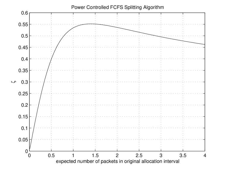
Figure 7.7: Plot of $\zeta$ versus $\lambda\phi_{0}$.

The right hand side of (7.68), $\zeta$, is a function of $\lambda\phi_{0}$ and is plotted in Figure 7.7. We observe that $\zeta$ takes its maximum value at $\lambda\phi_{0}=1.4$. More precisely, $\zeta$ has a numerically evaluated maximum of $0.5518$ at $\lambda\phi_{0}=1.4$. If $\phi_{0}$ is chosen to be $\frac{1.4}{0.5518}=2.54$, then (7.68) is satisfied for all $\lambda<0.5518$. Thus, the expected time backlog decreases whenever it is initially larger than $\phi_{0}$, and we infer that the algorithm is stable for $\lambda<0.5518$. We have therefore proved the following result.

Proposition 7.4.5.

The maximum stable throughput of the PCFCFS algorithm is 0.5518.

7.5 Numerical Results

In our numerical experiments, we use values of system parameters that are commonly encountered in wireless networks [42]. We compare the performance of the following algorithms:

1. FCFS with uniform power $P_{1}$,

2. PCFCFS.

For each algorithm, the value of the initial allocation interval is chosen so as to achieve maximum stable throughput. For FCFS, maximum stable throughput occurs when its initial allocation interval, $\alpha_{0}=2.6$ [22]. From Section 7.4, the maximum throughput of PCFCFS occurs at $\phi_{0}=2.54$. Let $n_{suc}$ denote the number of successful packets in $[0,\tau)$ and $d_{i}$ denote the departure time of $i^{th}$ packet.

For a given set of system parameters, we compute the following performance metrics:

Throughput $$= \frac{n_{suc}}{\tau},$$ (7.69)

Average Delay $$= \frac{\sum_{i=1}^{n_{suc}}(d_{i}-a_{i})}{n_{suc}},$$ (7.70)

Average Power $$= \frac{\sum_{i=1}^{n_{suc}}\sum_{k=\lceil a_{i}\rceil}^{d_{i}}P_{i}(k)}{n_{suc}}.$$ (7.71)

Keeping all other parameters fixed, we observe the effect of increasing the arrival rate on the throughput, average delay and average power.

Parameter	Symbol	Value
communication threshold	$\gamma_{c}$	7 dB
noise power spectral density	$N_{0}$	-90 dBm
path loss exponent	$\beta$	4
transmitter-receiver distance	$D$	100 m
initial allocation interval of FCFS	$\alpha_{0}$	2.6 s
initial allocation interval of PCFCFS	$\phi_{0}$	2.54 s
algorithm operation time	$\tau$	$3\times 10^{5}$ s

Table 7.1: System parameters for performance evaluation of PCFCFS and FCFS algorithms.

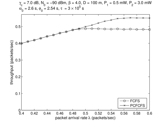
Figure 7.8: Throughput versus arrival rate for PCFCFS and FCFS algorithms.

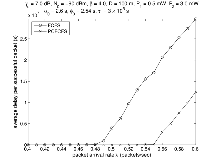
Figure 7.9: Average delay versus arrival rate for PCFCFS and FCFS algorithms.

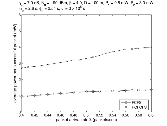
Figure 7.10: Average power versus arrival rate for PCFCFS and FCFS algorithms.

The system parameters for our numerical experiments are shown in Table 7.1. From (7.4) and (7.5), we obtain $P_{1}=0.50$ mW and $P_{2}=3.01$ mW. We vary the arrival rate $\lambda$ from $0.40$ to $0.60$ packets/s in steps of $0.01$. Figure 7.8 plots the throughput versus arrival rate for the PCFCFS and FCFS algorithms. Figure 7.9 plots the average delay per successful packet versus arrival rate for both the algorithms. Finally, Figure 7.10 plots the average power per successful packet versus arrival rate for both the algorithms.

For arrival rates exceeding $0.56$, the throughput of PCFCFS is less than the arrival rate (Figure 7.8) and the average delay of PCFCFS increases rapidly (Figure 7.9), which leads to a substantial increase in the number of backlogged packets and system instability. Hence, the maximum stable throughput of PCFCFS is between $0.55$ and $0.56$. Thus, Figures 7.8 and 7.9 corroborate our result that the maximum stable throughput of PCFCFS is $0.5518$ (see Section 7.4).

For both PCFCFS and FCFS, the departure rate (throughput) equals the arrival rate for all arrival rates up to 0.487 (Figure 7.8). Hence, both these algorithms are stable for arrival rates below 0.487. For arrival rates exceeding 0.487, the departure rate of FCFS is strictly lower than its arrival rate, leading to packet backlog and system instability. On the other hand, for PCFCFS, the departure rate still equals its arrival rate for arrival rates between 0.487 and 0.5518. In other words, the PCFCFS algorithm is stable for a higher range of arrival rates compared to FCFS algorithm. However, the PCFCFS algorithm becomes unstable for arrival rates exceeding 0.5518.

The PCFCFS algorithm achieves higher throughput and lower average delay than the FCFS algorithm, albeit at the cost of expending higher average power. For example, at $\lambda=0.55$, PCFCFS achieves $13.3\%$ higher throughput and $96.7\%$ lower average delay than FCFS, at the cost of $170\%$ higher power.

7.6 Conclusions

In this chapter, we have considered random access in wireless networks under the physical interference model. By recognizing that the receiver can successfully decode the strongest packet in presence of multiple transmissions, we have proposed PCFCFS, a splitting algorithm that modulates transmission powers of users based on observed channel feedback. PCFCFS achieves higher throughput and substantially lower delay than those of the well known FCFS algorithm with uniform transmission power. We show that the maximum stable throughput of PCFCFS is 0.5518. PCFCFS can be implemented in those scenarios where users are willing to trade some power for a substantial gain in throughput. Moreover, if users can estimate the arrival rate of packets, then they can employ FCFS algorithm for arrival rates up to 0.4871 and PCFCFS algorithm for higher arrival rates, thus leading to further reduction in average transmission power.

Chapter 8 Flow Control: An Information Theory Viewpoint

This thesis has so far explored various aspects of link scheduling in wireless networks. An equally interesting problem is to analyze flow control. We formulate the problem of controlling the rate of packets at the ingress of a packet network (possibly a wireless link) so as to maximize the mutual information between a source and a destination. We discuss various nuances of the problem and describe related work. We then derive the maximum entropy of a packet level flow that conforms to linearly bounded traffic constraints, by taking into account the covert information present in the randomness of packet lengths. Our results provide insights towards the design of flow control mechanisms employed by an Internet Service Provider (ISP).

The rest of the chapter is organized as follows. In Section 8.1, we define the problem of information theoretic analysis of flow control in a packet network. In Section 8.2, we introduce a Generalized Token Bucket Regulator (GTBR) as our flow control mechanism. The concepts of flow entropy and information utility are defined in Section 8.3. We formulate the problem of determining the GTBR with maximum information utility in Section 8.4. In Section 8.5, we derive a necessary condition for the optimal GTBR and compute its parameters. We explain the results from an information theoretic viewpoint in Section 8.6 and discuss the implications of our work in Section 8.7.

8.1 System Model

Figure 8.1: Flow control of a source’s packets over a packet network.

Our system model is shown in Figure 8.1, wherein a source sends packets to a destination over a packet-switched network (possibly a wireless network). The packets transmitted by the source are regulated (policed) by a flow control mechanism at the ingress of the network. We are interested in the packet probability distribution that maximizes the mutual information between the source and the destination. In other words, given the description of the flow control mechanism and the stochastic characterization of the packet network, we seek the maximum amount of information (in the Shannon sense) that can be transmitted from the source to the destination.

The problem can be stated as:

$$\max_{\mathbf{p}_{X}}I(X;Y),$$ (8.1)

where

$$X =$$ random variable representing randomness in packet contents, lengths

$$\mbox{and timings at the source},$$

$$y =$$ random variable representing randomness in packet contents, lengths

$$\mbox{and timings at the destination},$$

$$\mathbf{p}_{X} = \mbox{probability distribution of $X$}.$$

(8.1) can be simplified to:

$$\max_{\mathbf{p}_{X}}\big{(}H(X)-H(X|Y)\big{)}.$$ (8.2)

Thus, to maximize the information transfer from the source to the destination, we not only have to characterize the entropy of the source’s packets $H(X)$, but also the conditional entropy of the source’s packets given the packets received at the destination $H(X|Y)$.

We state the following remarks about our problem formulation:

1. It is well-known that, in a packet-switched network, information can be transmitted not only by the contents, but also by the lengths and timings of packets. [20] is perhaps the first work to recognize this fact. Information transmitted by the lengths and timings of packets is referred to as covert information or side information. The channel that is used to convey covert information is called covert channel. Covert channels have been investigated in [20], [21], [90].

2. By flow control, we mean a rate control mechanism that regulates the packets transmitted by a source (subscriber) at the ingress of a network. Note that we do not consider end-to-end flow control mechanisms such as Transmission Control Protocol (TCP). For simplicity, we consider a flow control mechanism that is described by a linearly bounded service curve [91].

3. In the packet network, packets can be received incorrectly at the destination due to fluctuations in the channel, like that in a wireless channel. We assume the existence of link layer mechanisms such as Forward Error Correction (FEC) which ensure that all packets are correctly received at the destination.

The packet network shown in Figure 8.1 only guarantees that the contents and lengths of the packets transmitted by the source are the same as those at the destination. However, the network can arbitrarily vary the timings between packets. Equivalently, the network can highly distort the covert timing information carried by the packets.

Taking a cue from this, we only take into account information that is carried by the contents and lengths of the packets. Consequently, the probability distribution of packet contents and lengths at the destination is the same as that at the source. Hence, $H(X|Y)=0$ and (8.2) simplifies to

$$\max_{\mathbf{p}_{X}}H(X).$$ (8.3)

In other words, we seek the probability distribution of packet contents and lengths that maximize the source entropy $H(X)$.

Typically, the entity that owns a network, say an Internet Service Provider (ISP), implements certain mechanisms to ensure that packets transmitted by a subscriber are not lost in the network. However, to allocate network resources efficiently and guarantee zero loss of packets, the entity also mandates that the aggregate traffic of a subscriber be upper bounded by an envelope or a service curve. For example, the entity can mandate that the aggregate traffic of the subscriber be linearly bounded. A linearly bounded service curve can be implemented by a class of regulators known as token bucket regulators.

Figure 8.2: Token bucket regulation of a source’s packets over a packet network.

The system model that we analyze incorporates a Token Bucket Regulator (TBR) and is shown in Figure 8.2. A source transmits packets to a destination over a network, where every packet consists of an integer number of bits. The packets transmitted by the source are regulated by a TBR or leaky bucket regulator [92]. Intuitively, the regulator collects tokens in a bucket of depth $B$, which fills up at a certain rate $r$. Each token corresponds to the permission to transmit one bit into the network. The packets to be transmitted by the source accumulate in its data buffer over time. If there is a packet of length $n$ bits in the data buffer at a given time, then it can be sent into the network only if $n\leqslant B+r$. If the packet is transmitted, then $n$ tokens are depleted from the token bucket.

A TBR can be used to smoothen the bursty nature of a subscriber’s traffic. We assume that the network is owned by an ISP. From a Quality of Service (QoS) perspective, a TBR can be considered to be a part of the Service Level Agreement (SLA) between a subscriber and an ISP. The SLA mandates that the ISP should provide end-to-end loss and delay guarantees to a subscriber’s packets, provided the traffic profile of the subscriber adheres to certain TBR constraints. Specifically, the onus of the ISP is to ensure that every packet of a conforming source successfully reaches its destination within a certain permissible delay.

The Standard Token Bucket Regulator (STBR), as defined by the Internet Engineering Task Force (IETF) and shown in Figure 8.2, enforces linear-boundedness on the flow. An STBR is characterized by its token increment rate $r$ and bucket depth $B$. We will be more general and consider a TBR in which the token increment rate and bucket depth (maximum burst size) can vary from slot to slot. Such a TBR, which we define as a Generalized Token Bucket Regulator (GTBR), can be used to regulate Variable Bit Rate (VBR) traffic from a source [93]. The continuous-time analogue of a GTBR is the time-varying leaky bucket shaper [94] in which the token rate and bucket depth parameters can change at specified time instants.

The idea is to develop the notion of information utility of a GTBR. Specifically, we derive the maximum information that a GTBR-conforming traffic flow can convey in a finite time interval, by taking into account the additional information present in the randomness of packet lengths. These aspects are further elucidated in subsequent sections.

8.2 Generalized Token Bucket Regulator

In this section, we mathematically describe our system model and define a GTBR. We also explain the differences between our system model and those considered in existing literature.

Figure 8.3: Relative time instants of parameters defined in (8.4).

Consider a system in which time is divided into slots and a source which has to complete its data transmission within $S$ slots. In our discrete-time model, we will evaluate the system at time instants $0,1,\ldots,S-1,S$. Slot $k$ is defined to be the time interval $[k,k+1)$, i.e., data transmission commences with slot 0 and terminates with slot $(S-1)$.

The traffic from the source is regulated by a GTBR. We define:

$$r_{k} = \mbox{token increment for slot $k$},$$

$$B_{k} = \mbox{bucket depth for slot $(k+1)$},$$

$$\ell_{k} = \mbox{length of packet (in bits) transmitted in slot $k$},$$

$$u_{k} = \mbox{residual tokens at start of slot $k$}.$$ (8.4)

$r_{k}$, $B_{k}$, $\ell_{k}$ and $u_{k}$, whose relative time instants are shown in Figure 8.3, are all non-negative integers. Let ${\mathbf{r}}:=(r_{0},r_{1},\ldots,r_{S-1})$ denote the token increment sequence and ${\mathbf{B}}:=(B_{0},B_{1},\ldots,B_{S-2})$ denote the bucket depth sequence. The system starts with zero tokens. So, $u_{0}=0$. A GTBR with the above parameters is denoted as $\mathcal{R}_{g}(S,\mathbf{r},\mathbf{B})$.

The constraints imposed by $\mathcal{R}_{g}(S,\mathbf{r},\mathbf{B})$ on the packet lengths is

$$\ell_{i}\leqslant u_{i}+r_{i}\;\;\forall\;\;i=0,1,\ldots,S-1.$$ (8.5)

If (8.5) is satisfied, then $\mathbf{\ell}=(\ell_{0},\ell_{1},\ldots,\ell_{S-1})$ is a conforming packet length vector and the number of residual tokens will evolve according to

$$u_{0} = 0,$$

$$u_{i+1} = \min(u_{i}+r_{i}-\ell_{i},B_{i})\;\;\forall\;\;i=0,1,\ldots,S-2,$$

$$u_{S} = u_{S-1}+r_{S-1}-\ell_{S-1}.$$ (8.6)

(8.6) is referred to as the token evolution equation.

Note that if $r_{i}=r$ $\forall$ $i=0,1,\ldots,S-1$ and $B_{i}=B$ $\forall$ $i=0,1,\ldots,S-2$, then the GTBR $\mathcal{R}_{g}(S,\mathbf{r},\mathbf{B})$ degenerates to the STBR $\mathcal{R}_{s}(S,r,B)$.

We should point out that our system model is similar to that of [95]. However, unlike [95], our traffic regulator is a deterministic mapping of an input sequence to an output sequence. Also, the rate of our regulator is defined by the average token increment rate and not by the peak rate.

The system model encompasses that of [90], wherein the authors have derived the information utility of an STBR and suggested a pricing viewpoint for its application. Our interest, however, is more theoretical. Specifically, we consider an STBR as a special case of a GTBR and describe a framework for their information-theoretic comparison. The main objective is to investigate whether a GTBR can achieve higher flow entropy than an STBR and explain the properties of entropy-maximizing GTBRs. These aspects are addressed in the following sections.

8.3 Notion of Information Utility

In this section, we introduce the concept of information utility of a GTBR. We derive the entropy of a flow that is regulated by a GTBR by considering the information present in the contents and lengths of the packets. We formulate the problem of computing the maximum flow entropy and subsequently describe a technique to compute the information utility of the GTBR.

Consider a source which has a large amount of data to send and whose traffic is regulated by a GTBR. We seek to maximize the information that the source can convey to the destination in the given time interval or the entropy present in the source traffic flow in an information-theoretic sense. For a given transmission interval $S$, token increment sequence $\mathbf{r}$ and bucket depth sequence $\mathbf{B}$, the maximum entropy achievable by any flow which is constrained by the GTBR $\mathcal{R}_{g}(S,\mathbf{r},\mathbf{B})$ is termed as the information utility of the GTBR $\mathcal{R}_{g}(\cdot)$.

The source can send information to its destination via two channels:

1. Overt channel: The contents of each packet. Let $\ell_{i}$ denote the length of a packet in bits. The value of each bit is $0$ or $1$ with equal probability and is independent of the values taken by the preceding and succeeding bits. Thus, this packet contributes $\ell_{i}$ bits of information.

2. Covert channel: We consider the length of a packet as an event and associate a probability with it. Thus, side information is transmitted by the randomness in the packet lengths.

The joint entropy of i. and ii. is the sum of their entropies.

During any slot $k$, the only method by which past transmissions can constrain the rest of the flow is by the residual number of tokens $u_{k}$. So, $u_{k}$ captures the state of the system. The key observation is that the future entropy depends only on the token bucket level $u_{k}$ in slot $k$. Hence, entropy is a function of system state $u_{k}$ and is denoted by $H_{k}(u_{k})$.

During slot $S$, the source signals the termination of the current flow by transmitting a special string of bits (flag). The information transmitted by this fixed sequence of bits is zero. Thus

$$H_{S}(u_{S}) = 0\;\;\forall\;u_{S}.$$ (8.7)

For a given state $u_{k}$ of the system, if a packet of length $\ell_{k}$ bits is transmitted with probability $p_{\ell_{k}}(u_{k})$, then

1. The overt information transmitted is $\ell_{k}$ bits,

2. As the event occurs with probability $p_{\ell_{k}}(u_{k})$, the covert information transmitted is $(-\log_{2}p_{\ell_{k}}(u_{k}))$ bits,

3. Since $\ell_{k}$ is random, $u_{k+1}$ is also random (from (8.6)). Thus, $H_{k+1}(u_{k+1})$ is also a random variable.

Adding all of the above and averaging it over all conforming packet lengths, we obtain the entropy in the current slot (stage)

$$H_{k}(u_{k}) = \sum_{\ell_{k}=0}^{u_{k}+r_{k}}p_{\ell_{k}}(u_{k})\Big{(}\ell_{k}-\log_{2}\big{(}p_{\ell_{k}}(u_{k})\big{)}+H_{k+1}\big{(}\min(u_{k}+r_{k}-\ell_{k},B_{k})\big{)}\Big{)}$$ (8.8)

$$\;\;\forall\;k=0,\ldots,S-1.$$

The equation above, which will be referred to as the flow entropy equation, intuitively states that the flow entropy of the current state is given by the sum of the entropy of the packet contents, the entropy of the packet lengths and the flow entropy of possible future states in the next slot. Note that (8.8) is similar to the backward recursion equation from dynamic programming [96]. Finally, the packet length probabilities must satisfy

$$\sum_{\ell_{k}=0}^{u_{k}+r_{k}}p_{\ell_{k}}(u_{k}) = 1\;\;\forall\;k=0,\ldots,S-1.$$ (8.9)

Let ${\mathbf{p}}_{k}(u_{k})=\left(p_{0}(u_{k}),p_{1}(u_{k}),\cdots,p_{u_{k}+r_{k}}(u_{k})\right)$ denote the vector of packet length probabilities for slot $k$ with $u_{k}$ residual tokens. The dependence of $p_{\ell_{k}}$ and ${\mathbf{p}}_{k}$ on $u_{k}$ is assumed to be understood and is not always stated explicitly. So, ${\mathbf{p}}_{k}=\left(p_{0},p_{1},\cdots,p_{u_{k}+r_{k}}\right)$.

Our objective is to determine the sequence of probability mass functions $({\mathbf{p}}_{S-1}^{*}$, ${\mathbf{p}}_{S-2}^{*}$, $\cdots$, ${\mathbf{p}}_{0}^{*})$ which maximizes the flow entropy $H_{0}(0)$ for a given GTBR $\mathcal{R}_{g}(S,\mathbf{r},\mathbf{B})$. From (8.7)

$$H_{S}^{*}(u_{S}) = 0.$$ (8.10)

From (8.8)

$$H_{k}(u_{k}) = \sum_{\ell_{k}=0}^{u_{k}+r_{k}}p_{\ell_{k}}\Big{(}\ell_{k}-\log_{2}(p_{\ell_{k}})+H_{k+1}^{*}\big{(}\min(u_{k}+r_{k}-\ell_{k},B_{k})\big{)}\Big{)}$$ (8.11)

$$\;\;\forall\;k=0,1,\ldots S-1.$$

Given $H_{k+1}^{*}(u_{k+1})$ $\forall$ $u_{k+1}$, there exists an optimum probability vector ${\mathbf{p}}_{k}^{*}=(p_{0}^{*},p_{1}^{*},\ldots,p_{u_{k}+r_{k}}^{*})$ which maximizes the flow entropy $H_{k}(u_{k})$, i.e.,

$$H_{k}^{*}(u_{k}) = \sum_{\ell_{k}=0}^{u_{k}+r_{k}}p_{\ell_{k}}^{*}\Big{(}\ell_{k}-\log_{2}(p_{\ell_{k}}^{*})+H_{k+1}^{*}\big{(}\min(u_{k}+r_{k}-\ell_{k},B_{k})\big{)}\Big{)}$$ (8.12)

$$\;\;\forall\;k=0,1,\ldots,S-1.$$

Thus, the problem of computing the entire sequence of probability vectors $(\mathbf{p}_{S-1}^{*}$, $\mathbf{p}_{S-2}^{*}$, $\cdots$, $\mathbf{p}_{0}^{*})$ decouples into a sequence of subproblems. The subproblem for slot $k$ is: Given the function $H_{k+1}^{*}(u_{k+1})\;\forall\;u_{k+1}$, determine the probability vector ${\mathbf{p}}_{k}=(p_{0},p_{1},\ldots,p_{u_{k}+r_{k}})$ so as to

maximize $$\sum_{\ell_{k}=0}^{u_{k}+r_{k}}p_{\ell_{k}}\Big{(}\ell_{k}-\log_{2}(p_{\ell_{k}})+H_{k+1}^{*}\big{(}\min(u_{k}+r_{k}-\ell_{k},B_{k})\big{)}\Big{)},$$

subject to $$\sum_{\ell_{k}=0}^{u_{k}+r_{k}}p_{\ell_{k}}=1.$$ (8.13)

(8.13) is an equality-constrained optimization problem and can be solved using the technique of Lagrange multipliers [97]. Define the Lagrangian

$${\mathcal{L}}({\mathbf{p}}_{k},\lambda_{k}) = \sum_{\ell_{k}=0}^{u_{k}+r_{k}}p_{\ell_{k}}\Big{(}\ell_{k}-\log_{2}(p_{\ell_{k}})+H_{k+1}^{*}\big{(}\min(u_{k}+r_{k}-\ell_{k},B_{k})\big{)}\Big{)}$$ (8.14)

$${}+\lambda_{k}\bigg{(}\sum_{\ell_{k}=0}^{u_{k}+r_{k}}p_{\ell_{k}}-1\bigg{)}.$$

At the optimal point $({\mathbf{p}}_{k}^{*},\lambda_{k}^{*})$, we must have

$$\left.\frac{\partial{\mathcal{L}}}{\partial p_{\ell_{k}}}\right|\begin{array}[]{c}\\ ({\mathbf{p}}_{k}^{*},\lambda_{k}^{*})\end{array} = 0\;\;\;\;\forall\;\;0\leqslant\ell_{k}\leqslant u_{k}+r_{k},$$ (8.17)

$$\left.\frac{\partial{\mathcal{L}}}{\partial\lambda_{k}}\right|\begin{array}[]{c}\\ ({\mathbf{p}}_{k}^{*},\lambda_{k}^{*})\end{array} = 0.$$ (8.20)

Solving (8.20) yields

$$\sum_{\ell_{k}=0}^{u_{k}+r_{k}}p_{\ell_{k}}^{*}(u_{k}) = 1,$$ (8.21)

which is (8.9) for the case of optimal probabilities. Solving (8.17), we obtain

$$p_{\ell_{k}}^{*}(u_{k}) = 2^{\ell_{k}-\log_{2}e+H_{k+1}^{*}(\min(u_{k}+r_{k}-\ell_{k},B_{k}))+\lambda_{k}^{*}(u_{k})}\;\;\forall\;\;0\leqslant\ell_{k}\leqslant u_{k}+r_{k}.$$ (8.22)

From (8.21) and (8.22), the optimal Lagrange multiplier is given by

$$\lambda_{k}^{*}(u_{k})=\log_{2}e-\log_{2}\bigg{(}\sum_{\ell_{k}=0}^{u_{k}+r_{k}}2^{\ell_{k}+H_{k+1}^{*}(\min(u_{k}+r_{k}-\ell_{k},B_{k}))}\bigg{)}.$$ (8.23)

From (8.22) and (8.23), the optimum packet length probability is given by

$$p_{\ell_{k}}^{*}(u_{k}) = \frac{2^{\ell_{k}+H_{k+1}^{*}(\min(u_{k}+r_{k}-\ell_{k},B_{k}))}}{\sum_{\alpha_{k}=0}^{u_{k}+r_{k}}2^{\alpha_{k}+H_{k+1}^{*}(\min(u_{k}+r_{k}-\alpha_{k},B_{k}))}}.$$ (8.24)

From (8.12) and (8.24), we finally obtain

$$H_{k}^{*}(u_{k}) = \log_{2}\bigg{(}\sum_{\ell_{k}=0}^{u_{k}+r_{k}}2^{\ell_{k}+H_{k+1}^{*}(\min(u_{k}+r_{k}-\ell_{k},B_{k}))}\bigg{)}.$$ (8.25)

(8.25) will be referred to as the optimal flow entropy equation.

The information utility of the GTBR $\mathcal{R}_{g}(S,\mathbf{r},\mathbf{B})$ is defined to be $H_{0}^{*}(0)$, the maximum flow entropy. $H_{0}^{*}(0)$ is computed by starting with $H_{S}^{*}(u_{S})=0$, and using (8.25) to compute the optimal flow entropy $H_{k}^{*}(u_{k})$ for all $u_{k}$ and then proceeding backward recursively for $k=S-1,S-2,\ldots,0$.

8.4 Problem Formulation

Having developed a method to compute the information utility of a GTBR in Section 8.3, we seek answers to the following questions:

1. Can a GTBR achieve higher information utility than that of an STBR?

2. If yes, what is the increase in information utility?

For the information-theoretic comparison of a GTBR ${\mathcal{R}}_{g}(S,{\mathbf{r}},{\mathbf{B}})$ and an STBR ${\mathcal{R}}_{s}(S^{\prime},r,B)$, we impose the following conditions:

1. $\mathcal{R}_{g}(\cdot)$ and $\mathcal{R}_{s}(\cdot)$ must operate over the same number of slots, i.e.,

   $$S = S^{\prime}.$$ (8.26)

2. The aggregate tokens of $\mathcal{R}_{g}(\cdot)$ and $\mathcal{R}_{s}(\cdot)$ must be equal, i.e.,

   $$\sum_{i=0}^{S-1}r_{i} = Sr.$$ (8.27)

3. The aggregate bucket depth of $\mathcal{R}_{g}(\cdot)$ must not exceed that of $\mathcal{R}_{s}(\cdot)$, i.e.,

   $$\sum_{i=0}^{S-2}{B_{i}} \leqslant (S-1)B.$$ (8.28)

4. The bucket depth of $\mathcal{R}_{s}(\cdot)$ cannot be very high compared to its token increment rate. To quantify this, we mandate

   $$2r\leqslant B\leqslant 5r.$$ (8.29)

5. The token increment rate of $\mathcal{R}_{g}(\cdot)$ in every slot must not exceed the bucket depth of $\mathcal{R}_{s}(\cdot)$, i.e.,

   $$r_{i} \leqslant B.$$ (8.30)

If Conditions 1, 2, 3, 4 and 5 are satisfied, then GTBR $\mathcal{R}_{g}(\cdot)$ and STBR $\mathcal{R}_{s}(\cdot)$ are said to be comparable to each other.

The optimal GTBR problem is formally stated as:
Given an STBR $\mathcal{R}_{s}(S,r,B)$, determine the token increment sequence $\mathbf{r}$ and bucket depth sequence $\mathbf{B}$ of a comparable GTBR $\mathcal{R}_{g}(S,\mathbf{r},\mathbf{B})$ so as to

maximize $$H_{0}^{*}(0),$$

subject to $$\sum_{i=0}^{S-1}r_{i} =Sr,$$ (8.31)

$$\sum_{i=0}^{S-2}B_{i} \leqslant(S-1)B.$$ (8.32)

Note that we are maximizing a real-valued function over two finite sequences of non-negative integers.

8.5 Results

In this section, we derive a necessary condition for the optimal GTBR in terms of aggregate bucket depth. We also compute the parameters of the optimal GTBR for some representative cases.

8.5.1 Analytical Result

Proposition 8.5.1.

For an optimal GTBR, equality must hold in (8.32), except when $S$ is small. In other words, if $\mathbf{B}^{*}$ is the bucket depth sequence of an optimal GTBR, it must satisfy

$$\sum_{i=0}^{S-2}B_{i}^{*} = (S-1)B.$$ (8.33)

Proof.

We prove by contradiction. Define $g_{k}(u)=2^{H_{k}^{*}(u)}$. Since $H_{k}^{*}(u)\geqslant 0$, $g_{k}(u)\geqslant 1$. From (8.25)

$$g_{k}(u) = \sum_{\ell=0}^{u+r_{k}}2^{\ell}g_{k+1}\big{(}\min(u+r_{k}-\ell,B_{k})\big{)}.$$ (8.34)

$g_{S-1}(u)=2^{u+r_{S-1}+1}-1$ is an increasing sequence in $u$. Using (8.34), we can show that $g_{k}(u)$ is an increasing sequence in $u$ $\forall$ $k=0,\ldots,S-1$. Let $\mu_{i}=$ maximum number of tokens possible in slot $i$. Thus

$$\mu_{0} = 0,$$ (8.35)

$$\mu_{i} = \min(\mu_{i-1}+r_{i-1},B_{i-1})\;\;\forall\;i=1,\ldots,S-1.$$ (8.36)

If $u_{i}\leqslant\mu_{i}$, then we say that state $u_{i}$ is reachable in slot $i$, otherwise it is unreachable.

Let $\mathcal{R}_{g}(S,\mathbf{r},\mathbf{B})$ be an optimal GTBR, for which equality does not hold in (8.32). Then $\sum_{i=0}^{S-2}B_{i}\leqslant(S-1)B-1$. Consider another GTBR $\mathcal{R}_{g}^{\prime}(S,\mathbf{r}^{\prime},\mathbf{B}^{\prime})$ with $\mathbf{r}^{\prime}=\mathbf{r}$ and $\mathbf{B}^{\prime}=(B_{0},\ldots,B_{k-1},B_{k}+1,B_{k+1},\ldots,B_{S-2})$ for some $k$. Let ${H_{k}^{\prime}}^{*}(u)$ denote the optimal flow entropy of $\mathcal{R}_{g}^{\prime}(\cdot)$ in slot $k$ with $u$ residual tokens. Define $g_{k}^{\prime}(u)=2^{{H_{k}^{\prime}}^{*}(u)}$. From (8.25)

$$g_{k}^{\prime}(u) = \sum_{\ell=0}^{u+r_{k}}2^{\ell}g_{k+1}^{\prime}\big{(}\min(u+r_{k}^{\prime}-\ell,B_{k}^{\prime})\big{)}.$$ (8.37)

$\mathbf{B}^{\prime}$ satisfies (8.32). $g_{i}^{\prime}(u)=g_{i}(u)$ $\forall$ $i=k+1,\ldots,S$ and $\forall$ $u$. Since $\min(u+r_{k}-\ell,B_{k}+1)\geqslant\min(u+r_{k}-\ell,B_{k})$, it follows that $g_{k}(\min(u+r_{k}-\ell,B_{k}+1))\geqslant g_{k}(\min(u+r_{k}-\ell,B_{k}))\geqslant 1$. If we determine a reachable state $u$ such that $g_{k}^{\prime}(u)>g_{k}(u)$, then $g_{0}^{\prime}(0)>g_{0}(0)$, since the flow entropy in slot $0$ is computed slot-by-slot as a linear sum of future possible flow entropies with positive weights. Thus, the problem now reduces to determining a slot $k$ and a reachable state $u$ such that $g_{k}^{\prime}(u)>g_{k}(u)$. One of the following must hold:

1. There exists an $i$ $\in$ $\{1,\ldots,S-1\}$ such that $\mu_{i}=B_{i-1}<\mu_{i-1}+r_{i-1}$, or

2. There is no $i$ such that $\mu_{i}=B_{i-1}<\mu_{i-1}+r_{i-1}$.

Case 1: Consider the smallest $i$ such that $\mu_{i}=B_{i-1}<\mu_{i-1}+r_{i-1}$. Substituting $k=i-1$ in (8.34), we obtain

$$g_{i-1}(u) = \sum_{\ell=0}^{u+r_{i-1}}2^{\ell}g_{i}\big{(}\min(B_{i-1},u+r_{i-1}-\ell)\big{)},$$

$$\therefore g_{i-1}(u) = \sum_{\ell=0}^{u+r_{i-1}-B_{i-1}-1}2^{\ell}g_{i}(B_{i-1})+\sum_{\ell=u+r_{i-1}-B_{i-1}}^{u+r_{i-1}}2^{\ell}g_{i}(u+r_{i-1}-\ell).$$ (8.38)

Substituting $k=i-1$ in (8.37), we obtain

$$g_{i-1}^{\prime}(u) = \sum_{\ell=0}^{u+r_{i-1}}2^{\ell}g_{i}\big{(}\min(B_{i-1}+1,u+r_{i-1}-\ell)\big{)},$$

$$\therefore g_{i-1}^{\prime}(u) = \sum_{\ell=0}^{u+r_{i-1}-B_{i-1}-1}2^{\ell}g_{i}(B_{i-1}+1)+\sum_{\ell=u+r_{i-1}-B_{i-1}}^{u+r_{i-1}}2^{\ell}g_{i}(u+r_{i-1}-\ell).$$ (8.39)

(8.38) and (8.39) hold only if

$$u+r_{i-1}-B_{i-1}-1\geqslant 0.$$ (8.40)

$u=\mu_{i-1}$ is a state which is reachable in the original system as well as in the primed system and satisfies (8.40). Since $g_{i}(u)$ is an increasing sequence in $u$, (8.38) and (8.39) imply $g_{i-1}^{\prime}(\mu_{i-1})>g_{i-1}(\mu_{i-1})$. Consequently, $g_{0}^{\prime}(0)>g_{0}(0)$.

Case 2: If no such $i$ exists, then we must have $B_{i}\geqslant r_{0}+\cdots+r_{i}$ $\forall$ $i=0,\ldots,S-2$. Adding these $(S-1)$ inequalities and using $r_{i}\leqslant B$ (from (8.30)),

$$\sum_{i=0}^{S-2}B_{i} \geqslant (Sr-r_{S-1})+(Sr-r_{S-1}-r_{S-2})+(Sr-r_{S-1}-r_{S-2}-r_{S-3})+\cdots,$$ (8.41)

$$\geqslant (Sr-B)+(Sr-2B)+(Sr-3B)+\cdots,$$

$$= S(S-1)r-\alpha B.$$ (8.42)

We cannot have $r_{i}=B$ $\forall$ $i$ (from (8.29), (8.30) and (8.31)). Thus, $\alpha$ cannot be of the order of $S^{2}$. Thus, the lower bound on $\sum_{i=0}^{S-2}B_{i}$ given by (8.41) and (8.42) is a loose lower bound. From (8.29), (8.32) and (8.42), $\sum_{i=0}^{S-2}B_{i}$ grows as $S^{2}$ and is upper-bounded by $5(S-1)r$, which is impossible (except when $S$ is small). So, we discard Case 2.

From the result of Case 1, ${H_{0}^{\prime}}^{*}(0)>H_{0}^{*}(0)$. So, our assumption that $\mathcal{R}_{g}(\cdot)$ is an optimal GTBR is incorrect. Therefore, equality must hold in (8.32) for every optimal GTBR. ∎

8.5.2 Numerical Results

STBR	optimal token increment	optimal bucket depth	information utility
parameters	sequence of GTBR	sequence of GTBR	$H_{s}$	$H_{g}^{*}$	percentage
($S$,$r$,$B$)	$\mathbf{r}^{*}$	$\mathbf{B}^{*}$	(bits)	(bits)	increase
(4,3,6)	(6 3 3 0)	(6 6 6)	20.04	20.92	4.4%
(4,3,7)	(6 4 2 0)	(6 8 7)	20.08	21.16	5.4%
(4,3,8)	(7 3 2 0)	(7 9 8)
	(8 3 1 0)	(8 9 7)	20.10	21.32	6.1%
(4,3,9)	(8 3 1 0)	(8 10 9)
	(9 2 1 0)	(9 10 8)	20.10	21.44	6.7%
(4,3,10)	(9 3 0 0)	(9 12 9)	20.10	21.51	7.0%
(4,3,11)	(10 2 0 0)	(10 12 11)
	(11 1 0 0)	(11 12 10)	20.10	21.54	7.2%
(4,3,12)	(12 0 0 0)	(12 12 12)	20.10	21.56	7.2%
(4,3,13)	(12 0 0 0)	(13 13 13)	20.10	21.56	7.2%
(4,4,8)	(8 4 4 0)	(8 8 8)	25.08	26.04	3.8%
(4,4,9)	(8 5 3 0)	(8 10 9)
	(9 4 3 0)	(9 10 8)	25.11	26.24	4.5%
(4,4,10)	(9 5 2 0)	(9 12 9)	25.13	26.39	5.0%
(4,4,12)	(11 4 1 0)	(11 14 11)	25.14	26.59	5.8%
(4,4,16)	(16 0 0 0)	(16 16 16)	25.14	26.70	6.2%
(4,5,10)	(10 5 5 0)	(10 10 10)	29.91	30.92	3.4%
(4,5,12)	(11 6 3 0)	(11 14 11)	29.96	31.24	4.3%
(4,6,12)	(11 7 6 0)	(11 13 12)
	(12 7 5 0)	(12 13 11)	34.60	35.66	3.1%
(5,3,6)	(6 3 3 3 0)	(6 6 6 6)	25.68	26.57	3.5%
(5,3,9)	(8 3 3 1 0)	(8 10 10 8)	25.88	27.33	5.6%
(5,3,12)	(11 2 2 0 0)	(11 13 13 11)	25.90	27.59	6.5%
(5,3,15)	(15 0 0 0 0)	(15 15 15 15)	25.90	27.64	6.7%
(6,2,4)	(4 2 2 2 2 0)	(4 4 4 4 4)	23.00	23.77	3.4%
(6,3,6)	(6 3 3 3 3 0)	(6 6 6 6 6)	31.33	32.23	2.9%

Table 8.1: Entropy-maximizing GTBR for given data transmission time, token rate and bucket depth of a comparable STBR.

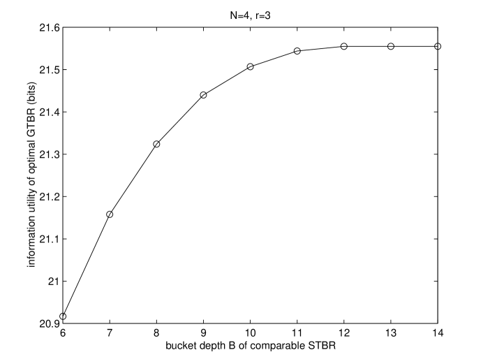
Figure 8.4: Information utility of GTBR vs. bucket depth of comparable STBR.

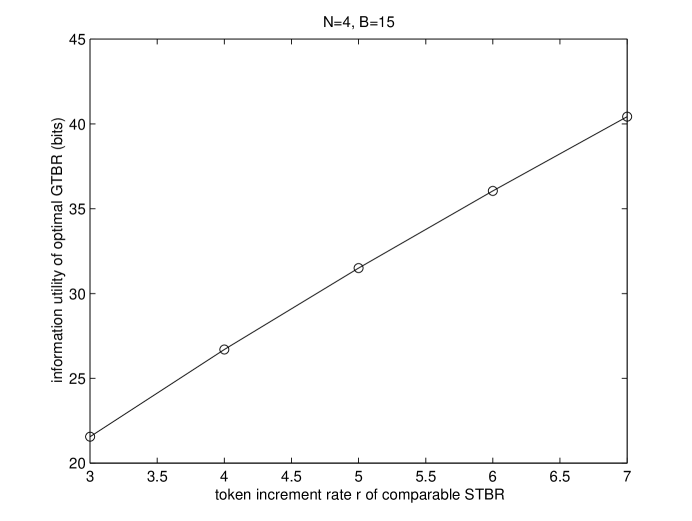
Figure 8.5: Information utility of GTBR vs. token increment rate of comparable STBR.

For a given data transmission time $S$, token increment sequence $\mathbf{r}$ and bucket depth sequence $\mathbf{B}$, we determine the optimal GTBR by exhaustive search over the reduced search space obtained from Proposition 8.5.1. Our computation results are shown in Table 8.1. $H_{s}$ and $H_{g}^{*}$ denote the information utility of the STBR $\mathcal{R}_{s}(S,r,B)$ and the optimal GTBR $\mathcal{R}_{g}(S,\mathbf{r}^{*},\mathbf{B}^{*})$ respectively. We also observe the variation in information utility of the optimal GTBR with important parameters of the comparable STBR, namely its bucket depth $B$ and token increment rate $r$. For a data transmission time of 4 slots and token increment rate of 3 bits, Figure 8.4 shows the variation of information utility of the GTBR versus the bucket depth of the comparable STBR. For a data transmission time of 4 slots and bucket depth of 15 bits, Figure 8.5 shows the variation of information utility of the GTBR versus the token increment rate of the comparable STBR.

Based on our computations, we draw the following inferences:

1. A generalized token bucket regulator can achieve higher information utility than that of a standard token bucket regulator. The increase in information utility is significant (up to 7.2%), especially for higher values of $B$.

2. The optimal bucket depth sequence $\mathbf{B}^{*}$ is uniform or near-uniform (the standard deviation is very small compared to the mean).

3. The optimal token increment sequence $\mathbf{r}^{*}$ is a decreasing sequence and is not uniform.

4. For a fixed data transmission time $S$ and token increment rate $r$:

   1. If $B=2r$, ${\mathbf{B}^{*}}$ is always uniform and ${\mathbf{r}^{*}}$ is uniform except for the terminal values.

   2. As $B$ increases from $2r$ to $\min(5,S)r$, the variance of ${\mathbf{r}^{*}}$ increases rapidly with a concentration of tokens in first few stages, the variance of ${\mathbf{B}^{*}}$ increases slowly, while $H_{g}^{*}$ initially increases and then saturates at some final value. $H_{g}^{*}$ is an increasing and concave sequence in $B$ (see Figure 8.4).

5. For a fixed data transmission time $S$ and bucket depth $B$, $H_{g}^{*}$ an increasing, highly linear and slightly concave sequence in $r$ (see Figure 8.5).

8.6 Information-Theoretic Interpretation

In this section, we provide explanations for empirical results in Section 8.5. The explanations are intuitive and rely on basic results from information theory.

Consider a system with $n$ states, where $p_{i}$ denotes the probability of state $i$ and $\sum_{i=1}^{n}p_{i}=1$. From classical information theory, system entropy $H$ increases with decreasing Kullback-Leibler distance between the given probability mass function (pmf) and the uniform pmf [98]. $H$ is maximized only if $p_{1}=\cdots=p_{n}=\frac{1}{n}$. Also, $H^{*}$ increases with $n$. Analogously, a GTBR can achieve higher information utility than that of an STBR because the pmfs of the packet lengths at each stage are more uniform and have a larger support. Recall that, for given $\mathbf{r}$ and $\mathbf{B}$, information utility is computed recursively using (8.6) and (8.25).

We argue that the optimal bucket depth sequence $\mathbf{B}^{*}$ must be uniform or near-uniform for maximum information utility. If $\mathbf{B}^{*}$ is neither uniform nor near uniform, then $B_{j}=\min_{i}B_{i}$ is much smaller than $B$. This restricts the range of values taken by $u_{j+1}$ and $\ell_{j+1}$ (from (8.5) and (8.6)). The support of packet length pmfs at stage $j+1$ is reduced, leading to lower flow entropy at stage $j+1$ and consequently lower information utility. Thus, ${\mathbf{B}^{*}}$ must be uniform or near-uniform to maximize the minimum support of packet length pmfs at each stage. In Table 8.1, the observation that $\min_{i}B_{i}^{*}=B-1$ or $\min_{i}B_{i}^{*}=B$ throughout corroborates our claim that $\mathbf{B}^{*}$ is near-uniform.

We argue that for maximum information utility, the optimal token increment sequence $\mathbf{r}^{*}$ must be a decreasing sequence, subject to $r_{i}\leqslant B_{i}$ for every $i$. If $r_{i}>B_{i}$ for any $i$, then a packet of length zero cannot be transmitted in slot $i$ (from (8.6)) and will have zero probability. This decreases the support of the packet length pmfs in slot $i$ and leads to lower information utility. More importantly, from (8.8),

$$H_{0}^{*}(0) = \sum_{\ell_{0}=0}^{r_{0}}p_{\ell_{0}}^{*}(0)\Big{(}\ell_{0}-\log_{2}\big{(}p_{\ell_{0}}^{*}(0)\big{)}+H_{1}^{*}\big{(}\min(r_{0}-\ell_{0},B_{0})\big{)}\Big{)}.$$ (8.43)

The major contribution to information utility $H_{0}^{*}(0)$ is from the support of the packet lengths $[0,r_{0}]$ and the pmf of the packet lengths $(\mathbf{p}_{0}^{*}(0))$, while the contribution from $H_{1}^{*}(\cdot)$ is relatively smaller. So, to maximize $H_{0}^{*}(0)$, $r_{0}$ should be allowed to take its maximum possible value, subject to $r_{0}\leqslant B_{0}$, and the pmf of the packet lengths should be close to the uniform pmf. The observation that $r_{0}=B_{0}$ consistently in Table 8.1 corroborates this. Also, a high value of $r_{0}$ leads to larger supports of packet length pmfs at intermediate and later stages. Similarly, the first few elements of $\mathbf{r}^{*}$ tend to take large values till the aggregate tokens are exhausted. However, their contribution to $H_{0}^{*}(0)$ is not as pronounced and equality may not hold in $r_{i}\leqslant B_{i}$. Thus, $\mathbf{r}^{*}$ must be a decreasing sequence and the first few elements of $\mathbf{r}^{*}$ tend to take their maximum possible values, subject to $r_{i}\leqslant B_{i}$, to achieve uniformity and larger supports of packet length pmfs at intermediate and later stages.

This “greedy” nature of $\mathbf{r}^{*}$ is evident when $S$ and $r$ are kept constant and $B$ increases (Result 6). A similar argument is applicable when $S$ and $B$ are kept constant and $r$ increases (Result 5). The only difference is that a unit increase in $r$ will necessarily increase $H_{g}^{*}$ by at least $S$ bits ($S$ bits are contributed by the packet contents alone, which also explains the dominant linear variation in Figure 8.5), while a unit increase in $B$ will increase $H_{g}^{*}$ only by an amount equal to the difference in covert information. The increase in covert information is positive only if the optimal token increment and bucket depth sequences (${\mathbf{r}^{*}}$ and ${\mathbf{B}^{*}}$) result in larger support and more uniformity for the packet length pmfs. Indeed, when $B$ increases beyond the maximum number of tokens possible at any stage ($\max_{i}\{\mu_{i}\}$), clamping the residual number of tokens at every stage becomes ineffective and the system behaves as if bucket depth constraints were not imposed at all (Figure 8.4).

8.7 Discussion

In this chapter, we have studied linearly bounded flows over a packet network. We considered a source whose traffic is regulated by a generalized token bucket regulator and which seeks to maximize the entropy of the resulting flow. Recognizing that the randomness in packet lengths acts as a covert channel in the network, the source can achieve maximum entropy by sizing its packets appropriately. We have formulated the problem of computing the GTBR with maximum information utility in terms of constrained token increment and bucket depth sequences. A GTBR can achieve higher information utility than that of a standard IETF token bucket regulator. Finally, we have information-theoretically interpreted the observation that an entropy-maximizing GTBR always has a near-uniform bucket depth sequence and a decreasing token increment sequence.

Chapter 9 Conclusions

The recent revolution in wireless communications has motivated researchers and engineers alike to design ever better wireless networks that deliver high data rates to users. The joint design of physical and MAC layers is the key to breaking the “bandwidth bottleneck” of wireless networks, which has been the primary inspiration for this thesis.

This thesis has focused on link scheduling in wireless mesh networks by taking into account physical layer characteristics. The assumption made throughout this thesis is that a packet is received successfully only if the SINR at the receiver exceeds a certain threshold, termed as communication threshold. The thesis has also discussed the complementary problem of flow control.

The first part of this thesis has considered link scheduling in STDMA wireless networks. The network is modeled by a finite set of store-and-forward nodes that communicate over a wireless channel characterized by propagation path loss. We have considered two nuances of the scheduling problem: point to point link scheduling wherein a transmitted packet is intended for a single neighbor only, and point to multipoint link scheduling wherein a transmitted packet is intended for all neighbors in the vicinity.

Specifically, in Chapter 2, we have introduced the system model of an STDMA wireless network. We have discussed two prevalent models for specifying the criteria for successful packet reception: the protocol interference model which mandates a “silence zone” around a receiver and is better suited to represent WLANs, and the physical interference model which mandates that the SINR at a receiver be no less than the communication threshold and is more appropriate to represent mesh networks. We have described the equivalence between a link schedule and the coloring of edges of a certain graph representation of the network, termed as communication graph. We have argued that STDMA link scheduling algorithms can be broadly categorized into three classes: those based entirely on a communication graph representation of the network, those based on communication graph and SINR threshold conditions and those based entirely on an SINR graph representation of the network. We have reviewed representative research papers from each of these classes. We have described limitations of algorithms that are based only on the communication graph. Subsequently, we have introduced spatial reuse as a performance metric that corresponds to aggregate network throughput.

Next, in Chapter 3, we have critically examined ArboricalLinkSchedule, a point to point link scheduling algorithm proposed in [16]. While this is one of the earlier works on link scheduling with nice theoretical properties, it could yield a higher schedule length in practice. Specifically, the methodology employed by ArboricalLinkSchedule is to represent the network by a communication graph, partition the graph into minimum number of subgraphs and color each subgraph in a greedy manner. We have modified the algorithm to reuse colors while coloring successive subgraphs of the communication graph. We have shown that the modified algorithm yields lower schedule length in practice, albeit at a cost of slightly higher running time complexity. Subsequently, we have proposed the ConflictFreeLinkSchedule algorithm that not only utilizes the communication graph, but also verifies SINR threshold conditions at receivers. We have demonstrated that the proposed algorithm achieves higher spatial reuse than existing algorithms, even under fading and shadowing channel conditions. We have argued that the running time complexity of the proposed algorithm is only marginally higher than those of existing algorithms.

Taking a step ahead, in Chapter 4, we have provided a somewhat different perspective on point to point link scheduling. For an STDMA network, we recognize that interferences between pairs of links can be embedded into edge weights and normalized noise powers at receivers of links can be embedded into vertex weights of a certain graph representation of the network, termed as SINR graph. We have then proposed SINRGraphLinkSchedule, a novel link scheduling algorithm that is based on the SINR graph. We have proved the correctness of the algorithm and shown that it has polynomial running time complexity. We have demonstrated that the proposed algorithm achieves high spatial reuse compared to algorithms which utilize a communication graph model of the network, including ConflictFreeLinkSchedule algorithm.

In Chapter 5, we have considered point to multipoint link scheduling and generalized the definition of spatial reuse for this scenario. We have proposed a scheduling algorithm based on a communication graph representation of the network and “neighbor-average” SINR threshold conditions. Moreover, we have demonstrated that the proposed algorithm achieves higher spatial reuse than existing algorithms, without any increase in running time complexity.

Overall, we have observed the tradeoff between accuracy of the network representation, spatial reuse and algorithm running time complexity in our successive results. For a more accurate network representation, higher spatial reuse is achieved, but at a cost of higher running time complexity. For example, since the SINR graph representation of an STDMA network is more accurate than the communication graph representation, SINRGraphLinkSchedule achieves higher spatial reuse than that of ConflictFreeLinkSchedule, but at a cost of increased running time complexity.

A summary of existing and proposed link scheduling algorithms investigated in the first part of the thesis is provided in Table 9.1.

Type of link	Wireless network	Existing	Proposed
scheduling	model	algorithms	algorithm
	communication graph	ArboricalLinkSchedule [16]	ALSReuseColors
			(Chapter 3)
Point	communication graph	GreedyPhysical [27]
to	and	TGSA [32]	ConflictFreeLinkSchedule
point	SINR conditions		(Chapter 3)
	SINR graph		SINRGraphLinkSchedule
			(Chapter 4)
Point	communication graph	BroadcastSchedule [16]
to	communication graph
multipoint	and		MaxAverageSINRSchedule
	SINR conditions		(Chapter 5)

Table 9.1: Link scheduling algorithms investigated in Chapters 3, 4 and 5.

The second part of this thesis has considered link scheduling in random access wireless networks. Specifically, it has focused on random access algorithms for wireless networks that take into account channel effects and SINR conditions at the receiver.

In Chapter 6, we have reviewed representative research papers on such random access techniques. We have also motivated the use of variable transmission power in random access wireless networks.

Subsequently, in Chapter 7, we have investigated a random access scenario wherein multiple transmitters (users) attempt to communicate with a single receiver over a wireless channel characterized by propagation path loss. We have assumed that the receiver is capable of power based capture and proposed an interval splitting algorithm that varies transmission powers of users based on their arrival times and quaternary channel feedback. We have modeled the algorithm dynamics by a Discrete Time Markov Chain and consequently shown that its maximum stable throughput is 0.5518. We have demonstrated that the proposed algorithm has higher throughput and lower delay than the FCFS interval splitting algorithm with uniform transmission power.

The third and final part of this thesis has considered information-theoretic analysis of flow control in packet networks. We have defined the problem of maximizing the information carried by packets from a source to a destination, subject to a flow control mechanism at the ingress of the network. We have considered a linearly bounded flow and focused on the information carried by the randomness in packet contents and lengths. Consequently, we have formulated the problem of maximizing the entropy of a packet level flow that is shaped by a generalized token bucket regulator. We have demonstrated that the optimal regulator has a decreasing token increment sequence and a near-uniform bucket depth sequence. Finally, we have provided information theoretic interpretations for these observations.

To sum it up, in this thesis, we have investigated both fixed and random access flavors of link scheduling problems in wireless networks from a physical layer viewpoint. Finally, we have discussed a flow control problem in packet networks.

Various avenues for further research have emerged from our investigations. We outline some possible directions for future work.

1. It would be interesting to derive approximation bounds of ConflictFreeLinkSchedule and SINRGraphLinkSchedule algorithms under reasonable assumptions on node deployment and interference regions. The assumptions and approximation techniques employed in [27] may provide some pointers in this direction.

2. Though distributed link scheduling algorithms for STDMA wireless networks under the protocol interference model have been proposed in [31], [99], the design of distributed link scheduling algorithms under the physical interference model remains a challenging problem.

3. Various generalizations of the PCFCFS algorithm are worth investigating. For example:

   1. Design a variable power splitting algorithm under the assumption that users are at unequal distances from the receiver and can adjust their minimum transmission powers accordingly.

   2. Design a splitting algorithm for the case when the receiver is capable of decoding more than one packet correctly (as in wideband systems) and the users can employ $n$ transmission power levels, where $n>2$.

   3. Analyze the throughput improvement in CSMA/CA based WLANs when power control is employed in conjunction with binary exponential backoff. The work done in [100] can be a useful starting point.

4. A challenging task would be to analyze the expected delay of the PCFCFS algorithm. A useful starting would be [101], [102], which have employed techniques to obtain upper and lowers bounds on the expected delay of the FCFS algorithm.

5. Our results in Chapter 8 show the existence of upper bounds on the entropy of regulated flows. It would be interesting to construct source codes which come close to this bound. Furthermore, it would be insightful to develop a rate-distortion framework for a generalized token bucket regulator, perhaps using the techniques employed in [95].

Appendix A Proofs of Limiting Transition Probabilities

According to L’Hôpital’s Rule, if $\lim_{x\rightarrow c}f(x)$ and $\lim_{x\rightarrow c}g(x)$ are both zero or are both $\pm\infty$ and, if $\lim_{x\rightarrow c}\frac{f(x)}{g(x)}$ has a finite value or if the limit is $\pm\infty$, then

$$\lim_{x\rightarrow c}\frac{f(x)}{g(x)} = \lim_{x\rightarrow c}\frac{f^{\prime}(x)}{g^{\prime}(x)}.$$ (A.1)

We will employ L’Hôpital’s Rule to prove (7.54) - (7.66)

In this appendix, we will only provide the proofs of (7.54), (7.55), (7.56) and (7.57). The proofs of (7.58) - (7.66) are similar to those of (7.54) - (7.57) and are omitted.

A.1 Proof of (7.54)

Proof.

In (7.25), substitute $G_{i}=x$. From (7.7), $G_{i-1}=2G_{i}=2x$. As $i\rightarrow\infty$, $G_{i}=2^{-i}\lambda\phi_{0}\rightarrow 0$. Thus, using L’Hôpital’s Rule successively, we obtain

$$\lim_{i\rightarrow\infty}P_{L_{i}^{\prime},R_{i}^{\prime}} = \lim_{x\rightarrow 0}\frac{(1-e^{-x})xe^{-x}}{1-(1+2x)e^{-2x}},$$

$$= \lim_{x\rightarrow 0}\frac{\frac{d}{dx}(xe^{-x}-xe^{-2x})}{\frac{d}{dx}(1-e^{-2x}-2xe^{-2x})},$$

$$= \lim_{x\rightarrow 0}\frac{e^{-x}+xe^{-x}-e^{-2x}}{4xe^{-2x}},$$

$$= \lim_{x\rightarrow 0}\frac{\frac{d}{dx}(e^{-x}+xe^{-x}-e^{-2x})}{\frac{d}{dx}(4xe^{-2x})},$$

$$= \lim_{x\rightarrow 0}\frac{2e^{-2x}-xe^{-x}}{4e^{-2x}-8xe^{-2x}},$$

$$\therefore\lim_{i\rightarrow\infty}P_{L_{i}^{\prime},R_{i}^{\prime}} = \frac{1}{2}.$$

∎

A.2 Proof of (7.55)

Proof.

In (7.26), substitute $G_{i}=x$. Thus, using $G_{i-1}=2x$ and applying L’Hôpital’s Rule successively, we obtain

$$\lim_{i\rightarrow\infty}P_{L_{i}^{\prime},L_{i+1}^{\prime}} = \lim_{x\rightarrow 0}\frac{(1-e^{-x}-xe^{-x})e^{-x}}{1-(1+2x)e^{-2x}},$$

$$= \lim_{x\rightarrow 0}\frac{\frac{d}{dx}(e^{-x}-e^{-2x}-xe^{-2x})}{\frac{d}{dx}(1-e^{-2x}-2xe^{-2x})},$$

$$= \lim_{x\rightarrow 0}\frac{e^{-2x}+2xe^{-2x}-e^{-x}}{4xe^{-2x}},$$

$$= \lim_{x\rightarrow 0}\frac{\frac{d}{dx}(e^{-2x}+2xe^{-2x}-e^{-x})}{\frac{d}{dx}(4xe^{-2x})},$$

$$= \lim_{x\rightarrow 0}\frac{e^{-x}-4xe^{-2x}}{4e^{-2x}-8xe^{-2x}},$$

$$\therefore\lim_{i\rightarrow\infty}P_{L_{i}^{\prime},L_{i+1}^{\prime}} = \frac{1}{4}.$$

∎

A.3 Proof of (7.56)

Proof.

In (7.27), substitute $G_{i}=x$. Thus, using $G_{i-1}=2x$ and applying L’Hôpital’s Rule successively, we obtain

$$\lim_{i\rightarrow\infty}P_{L_{i}^{\prime},C_{i+1}} = \lim_{x\rightarrow 0}\frac{\frac{x^{2}}{4}e^{-x}}{1-(1+2x)e^{-2x}},$$

$$= \lim_{x\rightarrow 0}\frac{\frac{d}{dx}(\frac{x^{2}}{4}e^{-x})}{\frac{d}{dx}(1-e^{-2x}-2xe^{-2x})},$$

$$= \lim_{x\rightarrow 0}\frac{\frac{1}{2}e^{-x}-\frac{x}{4}e^{-x}}{4e^{-2x}},$$

$$\therefore\lim_{i\rightarrow\infty}P_{L_{i}^{\prime},C_{i+1}} = \frac{1}{8}.$$

∎

A.4 Proof of (7.57)

Proof.

In (7.28), substitute $G_{i}=x$. Thus, using $G_{i-1}=2x$ and applying L’Hôpital’s Rule successively, we obtain

$$\lim_{i\rightarrow\infty}P_{L_{i}^{\prime},L_{i+1}} = \lim_{x\rightarrow 0}\frac{1-(1+x+\frac{x^{2}}{4})e^{-x}}{1-(1+2x)e^{-2x}},$$

$$= \lim_{x\rightarrow 0}\frac{\frac{d}{dx}(1-e^{-x}-xe^{-x}-\frac{x^{2}}{4}e^{-x})}{\frac{d}{dx}(1-e^{-2x}-2xe^{-2x})},$$

$$= \lim_{x\rightarrow 0}\frac{\frac{1}{2}-\frac{x}{2}}{4e^{-x}},$$

$$\therefore\lim_{i\rightarrow\infty}P_{L_{i}^{\prime},L_{i+1}} = \frac{1}{8}.$$

∎

Publications from the Thesis

1. A.D. Gore and A. Karandikar, “Entropy-Optimal Generalized Token Bucket Regulator,” in Proc. $12^{th}$ National Conference on Communications - NCC 2006, Indian Institute of Technology - Delhi, Joint Telematics Group of IITs/IISc, pp. 344-348, Jan. 2006.

2. A.D. Gore and A. Karandikar, “On High Spatial Reuse Broadcast Scheduling in STDMA Wireless Ad Hoc Networks,” in Proc. $13^{th}$ National Conference on Communications - NCC 2007, Indian Institute of Technology - Kanpur, Joint Telematics Group of IITs/IISc, pp. 74-78, Jan. 2007.

3. A.D. Gore and A. Karandikar, “Power Controlled FCFS Splitting for Wireless Networks,” in Proc. IEEE MILCOM, Orlando, Florida, USA, Oct. 2007.

4. A.D. Gore, S. Jagabathula and A. Karandikar, “On High Spatial Reuse Link Scheduling in STDMA Wireless Ad Hoc Networks,” in Proc. $50^{th}$ IEEE GLOBECOM, Washington, DC, USA, Nov. 2007.

5. N.P. Kumar, A.D. Gore and A. Karandikar, “Link Scheduling in STDMA Wireless Networks: A Line Graph Approach,” in Proc. $14^{th}$ National Conference on Communications - NCC 2008, Indian Institute of Technology - Bombay, Joint Telematics Group of IITs/IISc, pp. 108-111, Feb. 2008.

Bibliography

- [1] I. F. Akyildiz and X. Wang, “A Survey on Wireless Mesh Networks,” IEEE Communications Magazine, vol. 43, pp. S23–S30, Sept. 2005.
- [2] Cellular Operators Association of India. http://www.coai.in.
- [3] E. C. Efstathiou, P. A. Frangoudis, and G. C. Polyzos, “Stimulating Participation in Wireless Community Networks,” in Proc. IEEE INFOCOM, pp. 1–13, Apr. 2006.
- [4] TerraNet AB. http://www.terranet.se.
- [5] R. M. Metcalfe and D. R. Boggs, “Ethernet: Distributed Packet Switching for Local Computer Networks,” Communications of the ACM, vol. 19, pp. 395–404, July 1976.
- [6] LAN/MAN Standards Committee, IEEE Standard for Wireless LAN Medium Access Control (MAC) and Physical Layer (PHY) Specifications. IEEE Computer Society, June 2007. IEEE Std 802.11-2007.
- [7] LAN/MAN Standards Committee, IEEE Standard for Local and Metropolitan Area Networks: Part 16: Air Interface for Fixed Broadband Wireless Access Systems. IEEE Computer Society and IEEE Microwave Theory and Techniques Society, May 2004.
- [8] L. J. Cimini, “Analysis and Simulation of a Digital Mobile Channel using Orthogonal Frequency Division Multiplexing,” IEEE Transactions on Communications, vol. 33, pp. 665–675, July 1985.
- [9] A. R. Bahai, B. R. Saltzberg, and M. Ergen, Multi-Carrier Digital Communications: Theory and Applications of OFDM. Springer, 2nd ed., 2004.
- [10] D. Tse and P. Viswanath, Fundamentals of Wireless Communication. Cambridge University Press, 2005.
- [11] R. R. Choudhury, X. Yang, R. Ramanathan, and N. H. Vaidya, “On Designing MAC Protocols for Wireless Networks using Directional Antennas,” IEEE Transactions on Mobile Computing, vol. 5, pp. 477–491, May 2006.
- [12] E.-S. Jung and N. H. Vaidya, “A Power Control MAC Protocol for Ad Hoc Networks,” Wireless Networks, vol. 11, pp. 55–66, 2005.
- [13] J. So and N. H. Vaidya, “Multi-Channel MAC for Ad Hoc Networks: Handling Multi-Channel Hidden Terminals using a Single Transceiver,” in Proc. ACM MobiHoc, pp. 222–233, May 2004.
- [14] B. Sklar, “Rayleigh Fading Channels in Mobile Digital Communication Systems Part 1: Characterization,” IEEE Communications Magazine, vol. 35, pp. 90–100, July 1997.
- [15] P. Gupta and P. R. Kumar, “The Capacity of Wireless Networks,” IEEE Transactions on Information Theory, vol. 46, pp. 388–404, Mar. 2000.
- [16] S. Ramanathan and E. L. Lloyd, “Scheduling Algorithms for Multihop Radio Networks,” IEEE/ACM Transactions on Networking, vol. 1, pp. 166–177, Apr. 1993.
- [17] N. Abramson, “The ALOHA System - Another Alternative for Computer Communications,” in Proc. Fall Joint Computer Conf., pp. 281–285, AFIPS Press, 1970.
- [18] J. I. Capetanakis, “Tree Algorithms for Packet Broadcast Channels,” IEEE Transactions on Information Theory, vol. 25, pp. 505–515, Sept. 1979.
- [19] G. D. Nguyen, J. E. Wieselthier, and A. Ephremides, “Capture in Wireless Random Access Networks with Multiple Destinations and a Physical Channel Model,” in Proc. IEEE MILCOM, pp. 1200–1205, Oct. 2005.
- [20] R. G. Gallager, “Basic Limits on Protocol Information in Data Communication Networks,” IEEE Transactions on Information Theory, vol. 22, pp. 385–398, July 1976.
- [21] V. Anantharam and S. Verdu, “Bits Through Queues,” IEEE Transactions on Information Theory, vol. 42, pp. 4–18, Jan. 1996.
- [22] D. Bertsekas and R. Gallager, Data Networks. Prentice Hall, 1991.
- [23] R. Gupta, J. Musacchio, and J. Walrand, “Sufficient Rate Constraints for QoS Flows in Ad Hoc Networks,” Ad Hoc Networks, vol. 5, pp. 429–443, May 2007.
- [24] H. Lim, C. Lim, and J. C. Hou, “A Coordinate Based Approach for Exploiting Temporal Spatial Diversity in Wireless Mesh Networks,” in Proc. ACM MobiCom, pp. 14–25, Sept. 2006.
- [25] M. Alicherry, R. Bhatia, and E. Li, “Joint Channel Assignment and Routing for Throughput Optimization in Multiradio Wireless Mesh Networks,” in Proc. ACM MobiCom, pp. 58–72, Aug.-Sept. 2005.
- [26] K. Jain, J. Padhye, V. N. Padmanabhan, and L. Qiu, “Impact of Interference on Multihop Wireless Network Performance,” Wireless Networks, vol. 11, pp. 471–487, July 2005.
- [27] G. Brar, D. M. Blough, and P. Santi, “Computationally Efficient Scheduling with the Physical Interference Model for Throughput Improvement in Wireless Mesh Networks,” in Proc. ACM MobiCom, pp. 2–13, Sept. 2006.
- [28] R. Nelson and L. Kleinrock, “Spatial TDMA: A Collision Free Multihop Channel Access Protocol,” IEEE Transactions on Communications, vol. 33, pp. 934–944, Sept. 1985.
- [29] B. Hajek and G. Sasaki, “Link Scheduling in Polynomial Time,” IEEE Transactions on Information Theory, vol. 34, pp. 910–917, Sept. 1988.
- [30] M. Kodialam and T. Nandagopal, “Characterizing Achievable Rates in Multihop Wireless Mesh Networks with Orthogonal Channels,” IEEE/ACM Transactions on Networking, vol. 13, pp. 868–880, Aug. 2005.
- [31] T. Salonidis and L. Tassiulas, “Distributed Dynamic Scheduling for End-to-end Rate Guarantees in Wireless Ad Hoc Networks,” in Proc. ACM MobiHoc, pp. 145–156, May 2005.
- [32] A. Behzad and I. Rubin, “On the Performance of Graph Based Scheduling Algorithms for Packet Radio Networks,” in Proc. IEEE GLOBECOM, pp. 3432–3436, Dec. 2003.
- [33] J. Grönkvist and A. Hansson, “Comparison between Graph Based and Interference Based STDMA Scheduling,” in Proc. ACM MobiHoc, Oct. 2001.
- [34] M. Grötschel, L. Lovász, and A. Schrijver, “The Ellipsoid Method and its Consequences in Combinatorial Optimization,” Combinatorica, vol. 1, no. 2, pp. 169–197, 1981.
- [35] D. B. West, Introduction to Graph Theory. Prentice Hall, 2nd ed., 2000.
- [36] V. V. Vazirani, Approximation Algorithms. Springer, 2nd ed., 2004.
- [37] D. Hochbaum, Approximation Algorithms for NP-Hard Problems. Course Technology, 1996.
- [38] A. D. Gore, S. Jagabathula, and A. Karandikar, “On High Spatial Reuse Link Scheduling in STDMA Wireless Ad Hoc Networks,” in Proc. IEEE GLOBECOM, pp. 736–741, Nov. 2007.
- [39] T. Moscibroda and R. Wattenhofer, “The Complexity of Connectivity in Wireless Networks,” in Proc. IEEE INFOCOM, pp. 1–13, Apr. 2006.
- [40] T. Moscibroda, R. Wattenhofer, and A. Zollinger, “Topology Control Meets SINR: The Scheduling Complexity of Arbitrary Topologies,” in Proc. ACM MobiHoc, pp. 310–321, May 2006.
- [41] N. P. Kumar, A. D. Gore, and A. Karandikar, “Link Scheduling in STDMA Wireless Networks: A Line Graph Approach,” in Proc. National Conference on Communications, pp. 108–111, Feb. 2008.
- [42] T.-S. Kim, H. Lim, and J. C. Hou, “Improving Spatial Reuse through Tuning Transmit Power, Carrier Sense Threshold and Data Rate in Multihop Wireless Networks,” in Proc. ACM MobiCom, pp. 366–377, Sept. 2006.
- [43] V. F. Kolchin, B. A. Sevast’yanov, and V. P. Chistyakov, Random Allocations. V.H. Winston & Sons, 1978.
- [44] A. Madansky, “Inequalities for Stochastic Linear Programming Problems,” Management Science, vol. 6, pp. 197–204, 1960.
- [45] S. P. Dokov and D. P. Morton, “Higher Order Upper Bounds on the Expectation of a Convex Function.” Stochastic Programming E-Print Series, 2002. http://edoc.hu-berlin.de/series/speps/2002-8/PDF/8.pdf.
- [46] O. Somarriba, Multihop Packet Radio Systems in Rough Terrain. PhD thesis, Royal Institute of Technology, Stockholm, Sweden, Oct. 1995.
- [47] P. von Rickenbach, S. Schmid, R. Wattenhofer, and A. Zollinger, “A Robust Interference Model for Wireless Ad Hoc Networks,” in Proc. 5th Int. Workshop on Algorithms for Wireless, Mobile, Ad Hoc and Sensor Networks, Apr. 2005.
- [48] E. Arikan, “Some Complexity Results about Packet Radio Networks,” IEEE Transactions on Information Theory, vol. 30, pp. 681–685, July 1984.
- [49] H. N. Gabow and H. H. Westermann, “Forests, Frames and Games: Algorithms for Matroid Sums and Applications,” Algorithmica, vol. 7, pp. 465–497, Dec. 1992.
- [50] T. H. Cormen, C. E. Leiserson, and R. L. Rivest, Introduction to Algorithms. MIT Press, 2001.
- [51] M. L. Fredman and R. E. Tarjan, “Fibonacci Heaps and their Uses in Improved Network Optimization Algorithms,” Journal of the ACM, vol. 34, pp. 596–615, July 1987.
- [52] E. Lawler, Combinatorial Optimization: Networks and Matroids. Holt, Rinehart and Winston, 1976.
- [53] R. Motwani and P. Raghavan, Randomized Algorithms. Cambridge University Press, 1995.
- [54] A. Brzezinski, G. Zussman, and E. Modiano, “Enabling Distributed Throughput Maximization in Wireless Mesh Networks - A Partitioning Approach,” in Proc. ACM MobiCom, pp. 26–37, Sept. 2006.
- [55] T. Ramalingom, K. Thulasiraman, and A. Das, “A Matroid Theoretic Solution to an Assignment Problem in the Conformance Testing of Communication Protocols,” IEEE Transactions on Computers, vol. 49, pp. 317–330, Apr. 2000.
- [56] B. Petersen, “Investigating Solvability and Complexity of Linear Active Networks by Means of Matroids,” IEEE Transactions on Circuits and Systems, vol. 26, pp. 330–342, May 1979.
- [57] A. Goldsmith, Wireless Communications. Cambridge University Press, 2005.
- [58] P. Mutzel, T. Odenthal, and M. Scharbrodt, “The Thickness of Graphs: A Survey,” Graphs and Combinatorics, vol. 14, pp. 59–73, Mar. 1998.
- [59] L. Roberts, “ALOHA Packet System with and without Slots and Capture,” Computer Communications Review, vol. 5, pp. 28–42, Apr. 1975.
- [60] L. Kleinrock and F. A. Tobagi, “Packet Switching in Radio Channels: Part 1 - Carrier Sense Multiple Access Modes and Their Throughput-Delay Characteristics,” IEEE Transactions on Communications, vol. 23, pp. 1400–1416, Dec. 1975.
- [61] B. Hajek and T. van Loon, “Decentralized Dynamic Control of a Multiaccess Broadcast Channel,” IEEE Transactions on Automatic Control, vol. 27, pp. 559–569, June 1982.
- [62] R. L. Rivest, “Network Control by Bayesian Broadcast,” IEEE Transactions on Information Theory, vol. 33, pp. 323–328, May 1987.
- [63] H. Takagi and L. Kleinrock, “Throughput Analysis for Persistent CSMA Systems,” IEEE Transactions on Communications, vol. 33, pp. 627–638, July 1985.
- [64] J. L. Massey, “Conflict Resolution Algorithms and Random Access Communications,” in Multiuser Communications (G. Longo, ed.), Springer-Verlag, 1981.
- [65] M. L. Molle and G. C. Polyzos, “Conflict Resolution Algorithms and their Performance Analysis,” Tech. Rep. CS93-300, University of California, San Diego, USA, July 1993.
- [66] L. Tong, V. Naware, and P. Venkitasubramaniam, “Signal Processing in Random Access: A Cross Layer Perspective,” IEEE Signal Processing Magazine, vol. 21, pp. 29–39, Sept. 2004.
- [67] S. Verdu, Multiuser Detection. Cambridge University Press, 1998.
- [68] S. Ghez, S. Verdu, and S. C. Schwartz, “Stability Properties of Slotted ALOHA with Multipacket Reception Capability,” IEEE Transactions on Automatic Control, vol. 33, pp. 640–649, July 1988.
- [69] V. Naware, G. Mergen, and L. Tong, “Stability and Delay of Finite User Slotted ALOHA with Multipacket Reception,” IEEE Transactions on Information Theory, vol. 51, pp. 2636–2656, July 2005.
- [70] B. Hajek, A. Krishna, and R. O. LaMaire, “On the Capture Probability for a Large Number of Stations,” IEEE Transactions on Communications, vol. 45, pp. 254–260, Feb. 1997.
- [71] M. K. Tsatsanis, R. Zhang, and S. Banerjee, “Network Assisted Diversity for Random Access Wireless Networks,” IEEE Transactions on Signal Processing, vol. 48, pp. 702–711, Mar. 2000.
- [72] R. Zhang, N. D. Sidiropoulos, and M. K. Tsatsanis, “Collision Resolution in Packet Radio Networks using Rotational Invariance Techniques,” IEEE Transactions on Communications, vol. 50, pp. 146–155, Jan. 2002.
- [73] G. Dimic, N. D. Sidiropoulos, and L. Tassiulas, “Wireless Networks with Retransmission Diversity Access Mechanisms: Stable Throughput and Delay Properties,” IEEE Transactions on Signal Processing, vol. 51, pp. 2019–2030, Aug. 2003.
- [74] G. Dimic, N. D. Sidiropoulos, and R. Zhang, “Medium Access Control–Physical Cross-Layer Design,” IEEE Signal Processing Magazine, vol. 21, pp. 40–50, Sept. 2004.
- [75] X. Qin and R. Berry, “Exploiting Multiuser Diversity for Medium Access Control in Wireless Networks,” in Proc. IEEE INFOCOM, pp. 1084–1094, March-April 2003.
- [76] S. Adireddy and L. Tong, “Exploiting Decentralized Channel State Information for Random Access,” IEEE Transactions on Information Theory, vol. 51, pp. 537–561, Feb. 2005.
- [77] R.-H. Gau, “Performance Analysis of Slotted ALOHA in Interference Dominating Wireless Ad Hoc Networks,” IEEE Communications Letters, vol. 10, pp. 402–404, May 2006.
- [78] J. S. Lee and L. E. Miller, CDMA Systems Engineering Handbook. Artech House, 1998.
- [79] F. Baccelli, B. Blaszczyszyn, and P. Mühlethaler, “An ALOHA Protocol for Multihop Mobile Wireless Networks,” IEEE Transactions on Information Theory, vol. 52, pp. 421–436, Feb. 2006.
- [80] W. Navidi and T. Camp, “Stationary Distributions for the Random Waypoint Mobility Model,” IEEE Transactions on Mobile Computing, vol. 3, pp. 99–108, Jan.-Mar. 2004.
- [81] X. Qin and R. Berry, “Opportunistic Splitting Algorithms for Wireless Networks,” in Proc. IEEE INFOCOM, pp. 1662–1672, Mar. 2004.
- [82] K. J. Arrow, L. Pesotchinsky, and M. Sobel, “On Partitioning a Sample with Binary-Type Questions in Lieu of Collecting Observations,” Journal of the American Statistical Association, vol. 76, pp. 402–409, June 1981.
- [83] Y. Yu and G. B. Giannakis, “SICTA: A 0.693 Contention Tree Algorithm using Successive Interference Cancellation,” in Proc. IEEE INFOCOM, pp. 1908–1916, Mar. 2005.
- [84] B. Tsybakov, “Packet Multiple Access for Channel with Binary Feedback, Capture and Multiple Reception,” IEEE Transactions on Information Theory, vol. 50, pp. 1073–1085, June 2004.
- [85] A. Dua, “Power Controlled Random Access,” in Proc. IEEE ICC, pp. 3514–3518, June 2004.
- [86] R. J. Duffin, E. L. Peterson, and C. Zener, Geometric Programming - Theory and Application. John Wiley & Sons, 1967.
- [87] Y. E. Sagduyu and A. Ephremides, “Power Control and Rate Adaptation as Stochastic Games for Random Access,” in Proc. IEEE Conference on Decision and Control, pp. 4202–4207, Dec. 2003.
- [88] M. Zorzi, “Mobile Radio Slotted ALOHA with Capture and Diversity,” Wireless Networks, vol. 1, pp. 227–239, June 1995.
- [89] L. Georgiadis and P. Papantoni-Kazakos, “A Collision Resolution Protocol for Random Access Channels with Energy Detectors,” IEEE Transactions on Communications, vol. 30, pp. 2413–2420, Nov. 1982.
- [90] P. Shah and A. Karandikar, “Information Utility of Token Bucket Regulator,” Electronics Letters, vol. 39, pp. 581–582, Mar. 2003.
- [91] J.-Y. L. Boudec and P. Thiran, Network Calculus: A Theory of Deterministic Queuing Systems for the Internet. Springer, 2001.
- [92] S. Keshav, An Engineering Approach to Computer Networking. Addison Wesley Longman, 1997.
- [93] P. Shah and A. Karandikar, “Optimal Packet Length Scheduling for Regulated Media Streaming,” IEEE Communications Letters, vol. 7, pp. 409–411, Aug. 2003.
- [94] S. Giordano and J.-Y. L. Boudec, “On a Class of Time Varying Shapers with Application to the Renegotiable Variable Bit Rate Service,” Journal on High Speed Networks, vol. 9, pp. 101–138, June 2000.
- [95] C.-S. Chang, C.-C. Chao, and J. A. Thomas, “Fundamental Limits of Traffic Regulation and their Connections to Source Coding,” in Proc. IEEE Conference on Decision and Control, pp. 791–796, Dec. 1996.
- [96] D. P. Bertsekas, Dynamic Programming and Optimal Control. Athena Scientific, 2007.
- [97] D. P. Bertsekas, Nonlinear Programming. Athena Scientific, 1999.
- [98] T. M. Cover and J. A. Thomas, Elements of Information Theory. John Wiley & Sons, 1991.
- [99] P. Djukic and S. Valaee, “Distributed Link Scheduling for TDMA Mesh Networks,” in Proc. IEEE ICC, pp. 3823–3828, June 2007.
- [100] C. J. Colbourn, M. Cui, E. L. Lloyd, and V. R. Syrotiuk, “A Carrier Sense Multiple Access Protocol with Power Backoff (CSMA/PB),” Ad Hoc Networks, vol. 5, pp. 1233–1250, Nov. 2007.
- [101] J.-C. Huang and T. Berger, “Delay Analysis of Interval Searching Contention Resolution Algorithms,” IEEE Transactions on Information Theory, vol. 31, pp. 264–273, Mar. 1985.
- [102] J.-C. Huang and T. Berger, “Delay Analysis of 0.487 Contention Resolution Algorithms,” IEEE Transactions on Communications, vol. 34, pp. 916–926, Sept. 1986.