Resonant Cascaded Down-Conversion

Abstract

We analyze an optical parametric oscillator (OPO) in which cascaded down-conversion occurs inside a cavity resonant for all modes but the initial pump. Due to the resonant cascade design, the OPO present two $\chi^{(2)}$ level oscillation thresholds that are therefore remarkably lower than for a $\chi^{(3)}$ OPO. This is promising for reaching the regime of an effective third-order nonlinearity well above both thresholds. Such a $\chi^{(2)}$ cascaded device also has potential applications in frequency conversion to far infra-red regimes. But, most importantly, it can generate novel multi-partite quantum correlations in the output radiation, which represent a step beyond squeezed or entangled light. The output can be highly non-Gaussian, and therefore not describable by any semi-classical model.

I Introduction

Continuous-variable (CV) quantum information is an interesting flavor of quantum information (QI) book ; rmp . While easily implemented by use of well established quantum optics techniques, benefiting from large flow rates and broad spectral band, it has long been based on coherent states and linear Bogoliubov transformations (quadratic Hamiltonians) and therefore restricted to positive Wigner functions of Gaussian character. These states are not general enough for universal quantum information operationsllb . For instance, it has been shown that quantum computation based solely on Gaussian CV states can be efficiently simulated by a classical computer eff_cl_sim . Also, CV entanglement purification requires a Kerr-nonlinearity-based QND measurement duan or, in general, a non-Gaussian state plenio . However, it has also been shown that one-way quantum computing can be implemented using Gaussian cluster-state entanglement combined with non-CV (e.g., photon counting) measurements menicucci .

Recently, successful “degaussification" experiments, using homodyne detection conditioned on single-photon detection lvovsky ; wenger ; bellini ; polzik , have successfully generated negative Wigner functions from initial squeezed states. Here, we investigate different type of sources, which can produce non-Gaussian light directly. Theoretical studies of optical parametric oscillators (OPO), which are based on a single second-order optical nonlinearity ($\chi^{(2)}$) have shown non-Gaussian signatures to be rather scarce drummond_deg except in the case of the tripartite correlations between the three fields drummond_nondeg . An interesting approach is to use an optical nonlinearity of, at least, third order. This has been theoretically investigated felbinger ; braunstein ; hillery ; banaszek . In practice, a $\chi^{(3)}$ based OPO would have the problems of requiring a very large and possibly prohibitive input power threshold for downconversion, together with an even higher threshold for the onset of nonclassical effects, such as the formation of star states felbinger .

In this paper, we show how the use of a cavity-resonant cascade of second-order nonlinearities can yield a low-threshold OPO which possesses the effective behavior of a $\chi^{(3)}$ OPO in certain regimes and is more accessible experimentally. Note that related systems have been studied before, in the purely classical case and for completely different purposes, such as producing new tunable optical sources in the infrared moore or achieving optical phase-locking in a 3:1 frequency ratio for frequency metrology Zondy_PRA2001 ; Zondy_PRL2004 . Parametric amplifiers and oscillators have become a widely used, even standard part of the repertoire of laser physics and quantum optics Yar89 . Above the classical threshold points, these devices are a useful tool for frequency conversion. Below threshold, quantum effects dominate, leading to squeezing and entanglement. These devices that rely on non-resonant, nonlinear optics interactions have proved experimentally superior to other resonant or near-resonant alternatives, due to the fact that absorption is suppressed.

There are other possible quantum effects available, as well as direct down-conversion in the linear regime well below threshold. For example, exploration of non-equilibrium quantum criticality is possible near threshold. This results in large critical fluctuations and phase-transitions. The fluctuations in this case become non-Gaussian, but the dominant critical fluctuations have a rather classical character. Here, we explore another path to such non-Gaussian behavior, in which extremely nonclassical correlations are generated through the presence of a second down-conversion crystal placed inside the cavity. We show that this results in an intricate pattern of new phase-transitions at the classical level, in which there are two distinct threshold points. At the quantum level, below the first threshold, there are very strong triple correlations between the three down-converted modes, which have no classical analog.

This paper is structured as follows. In Section II, we explain the basic model and the theoretical phase-space techniques that are used here. In Section III, we present an analytical study of the system’s stationary solutions. In Section IV, we turn to a treatment of stability properties and fluctuations in one particular type of down-conversion scenario. In Section V, we give numerical simulations of more general cases which can also yield regimes of interest. These simulations demonstrate the stability regions, in the same spirit as was achieved for the $\chi^{(2)}$ OPO lugiato . We give conclusions in Section VI.

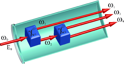
Figure 1: (Color online) Schematic of the resonant cascaded down-conversion system. A driving field, that is pumped at a frequency $\omega_{0}$ with amplitude $E_{0}$, enters a cavity that contains two $\chi^{(2)}$ nonlinear crystals. The first $\chi_{1}^{(2)}$ crystal down-converts the original mode $\hat{a}_{0}$ into two modes $\hat{a}_{1}$ and $\hat{a}_{2}$ with frequencies $\omega_{1}$ and $\omega_{2}$, respectively. Then the second mode $\hat{a}_{2}$ undergoes a further down-conversion, via the $\chi_{2}^{(2)}$ crystal, into the two modes $\hat{a}_{3}$ and $\hat{a}_{4}$ with frequencies $\omega_{3}$ and $\omega_{4}$, respectively.

II Analytical treatment

II.1 Cascaded parametric oscillator model

The model system for cascaded down-conversion consists of two quadratically nonlinear elements with nonlinearities $\chi_{1}$ and $\chi_{2}$ inside an optical cavity (c.f. Fig. 1). The cavity supports five resonant modes at frequencies $\omega_{i}$ ($i=0,1,...4$). The mode $\omega_{0}$ is the pump mode, driven by an external coherent driving field at the same frequency $\omega_{0}$. The cavity modes $\omega_{i}$ are described by creation and annihilation operators $\hat{a}_{i}^{\dagger}$ and $\hat{a}_{i}$ with commutation relations $[\hat{a}_{i},\hat{a}_{j}^{\dagger}]=\delta_{ij}$. The first nonlinear element converts the pump mode $\omega_{0}$ into the signal and idler modes $\omega_{1}$ and $\omega_{2}$ by means of nondegenerate parametric down-conversion, where $\omega_{0}=\omega_{1}+\omega_{2}$ ($\omega_{1}\neq\omega_{2}$). The second nonlinear crystal supports down-conversion of the mode $\omega_{2}$ into the second pair of signal and idler modes, $\omega_{3}$ and $\omega_{4}$, where $\omega_{2}=\omega_{3}+\omega_{4}$. We will call the field $\hat{a}_{2}$ at $\omega_{2}$ the “intermediate pump." The modes may decay via cavity losses at the respective rates $\gamma_{i}$, $i\in[0,4]$.

In the absence of the optical cavity, this interaction constitutes a cascade of quantum systems in the sense investigated by several authors before gardiner , where the second stage does not feed back to the first stage. Here, the situation is different precisely because of the cavity feedback, hence our use of the term resonant cascade throughout the paper. Within this frame, we will distinguish two situations: the first one is the nondegenerate resonant cascade, for which the fields $\hat{a}_{1}$, $\hat{a}_{3}$, and $\hat{a}_{4}$ are distinguishable (i.e.,  $\omega_{1}\neq\omega_{3}\neq\omega_{4}$, or having different polarizations or wave-vector directions). In this case, the only physical observable affected by both stages of the cascade is the intermediate pump $\hat{a}_{2}$. This is the case that will be investigated analytically, with additional simplifying hypotheses, and numerically, without those hypotheses. The second case is the degenerate resonant cascade, for which the signal fields are indistinguishable: $\hat{a}_{1}\equiv\hat{a}_{3}\equiv\hat{a}_{4}$ (and hence $\omega_{1}=\omega_{3}=\omega_{4}$). In that case the signal field and the intermediate pump interact in both nonlinear media and the dynamics are richer. That case will be explored by numerical simulations. Obviously, intermediate situations do also exist, e.g., $\omega_{1}=\omega_{3}\neq\omega_{4}$, but we will not consider them here.

II.2 Hamiltonian and equations of motion

The model Heisenberg-picture Hamiltonian for the system, in the rotating-wave approximation, is given by:

$$\hat{H}= \sum_{i=0}^{4}\hbar\omega_{i}\hat{a}_{i}^{\dagger}\hat{a}_{i}+i\hbar(E_{0}e^{-i\omega_{0}t}\hat{a}_{0}^{\dagger}-E_{0}^{\ast}e^{i\omega_{0}t}\hat{a}_{0})$$

$$+i\hbar\chi_{1}(\hat{a}_{0}\hat{a}_{1}^{\dagger}\hat{a}_{2}^{\dagger}-\hat{a}_{0}^{\dagger}\hat{a}_{1}\hat{a}_{2})+i\hbar\chi_{2}(\hat{a}_{2}\hat{a}_{3}^{\dagger}\hat{a}_{4}^{\dagger}-\hat{a}_{2}^{\dagger}\hat{a}_{3}\hat{a}_{4})$$

$$+\sum_{i=0}^{4}(\hat{a}_{i}\hat{\Gamma}_{i}^{\dagger}+\hat{a}_{i}^{\dagger}\hat{\Gamma}_{i})$$ (1)

Here, $E_{0}$ describes the complex amplitude of the driving field. The coupling constants $\chi_{1}$ and $\chi_{2}$ are proportional to the second-order susceptibilities of the two nonlinear elements, respectively. We assume that they are positive, without loss of generality, since phase factors can always be absorbed into the definitions of the mode functions and their operators. The operators $\hat{\Gamma}_{i}$ and $\hat{\Gamma}_{i}^{\dagger}$ describe the coupling of each intracavity mode to the reservoir of external modes. These give rise to the losses of the cavity modes $\omega_{i}$ at rates $\gamma_{i}$.

II.2.1 Master Equation

Transforming to an interaction picture in which all operators are transformed to rotating frames, i.e.,

$$\hat{a}_{j}(t)=\hat{a}_{j}e^{-i\omega_{j}t},$$ (2)

one can derive the following master equation for the system density operator $\hat{\rho}$ Louisell :

$$\frac{\partial\hat{\rho}}{\partial t} =[E_{0}\hat{a}_{0}^{\dagger}-E_{0}^{\ast}\hat{a}_{0},\hat{\rho}]+\chi_{1}[\hat{a}_{0}\hat{a}_{1}^{\dagger}\hat{a}_{2}^{\dagger}-\hat{a}_{0}^{\dagger}\hat{a}_{1}\hat{a}_{2},\hat{\rho}]$$

$$+\chi_{2}[\hat{a}_{2}\hat{a}_{3}^{\dagger}\hat{a}_{4}^{\dagger}-\hat{a}_{2}^{\dagger}\hat{a}_{3}\hat{a}_{4},\hat{\rho}]$$

$$+\sum_{i=0}^{4}\gamma_{i}(2\hat{a}_{i}\hat{\rho}\hat{a}_{i}^{\dagger}-\hat{\rho}\hat{a}_{i}^{\dagger}\hat{a}_{i}-\hat{a}_{i}^{\dagger}\hat{a}_{i}\hat{\rho}).$$ (3)

While in principle this master equation can be solved numerically in a number-state representation, in practice this is not possible. The complexity of the Hilbert space — especially for this five mode problem — is enormous, given any moderate number of photons present in the five interacting modes. Instead, we solve this problem using phase-space representation methods, such as the positive-P representationgen-p-rep .

II.3 Positive-P representation

Using the positive-P representation we can transform the master equation, Eq. (3), into a Fokker-Planck equation gen-p-rep expressed as:

$$\frac{\partial}{\partial t}P(\mathbf{\alpha},\mathbf{\alpha}^{+},t)= \left[\frac{\partial}{\partial\alpha_{0}}(\gamma_{0}\alpha_{0}-E_{0}+\chi_{1}\alpha_{1}\alpha_{2})\right.$$

$$+\frac{\partial}{\partial\alpha_{1}}(\gamma_{1}\alpha_{1}-\chi_{1}\alpha_{0}\alpha_{2}^{+})$$

$$+\frac{\partial}{\partial\alpha_{2}}(\gamma_{2}\alpha_{2}-\chi_{1}\alpha_{0}\alpha_{1}^{+}+\chi_{2}\alpha_{3}\alpha_{4})$$

$$+\frac{\partial}{\partial\alpha_{3}}(\gamma_{3}\alpha_{3}-\chi_{2}\alpha_{2}\alpha_{4}^{+})$$

$$+\frac{\partial}{\partial\alpha_{4}}(\gamma_{4}\alpha_{4}-\chi_{2}\alpha_{2}\alpha_{3}^{+})$$

$$+\frac{\partial^{2}}{\partial\alpha_{1}\partial\alpha_{2}}(\chi_{1}\alpha_{0})$$

$$\left.+\frac{\partial^{2}}{\partial\alpha_{3}\partial\alpha_{4}}(\chi_{2}\alpha_{2})+h.c.\right]P(\mathbf{\alpha},\mathbf{\alpha}^{+},t).$$ (4)

Here, $\mathbf{\alpha}\equiv(\alpha_{0},\alpha_{1},\alpha_{2},\alpha_{3},\alpha_{4})$ and $\mathbf{\alpha}^{+}\equiv(\alpha_{0}^{+},\alpha_{1}^{+},\alpha_{2}^{+},\alpha_{3}^{+},\alpha_{4}^{+})$ represent the sets of coherent state amplitudes $\alpha_{i}$ and $\alpha_{i}^{+}$ in the expansion of the density operator in terms of the positive $P$-representation, corresponding to the annihilation and creation operators $\hat{a}_{i}$ and $\hat{a}_{i}^{\dagger}$. We recall that in the positive $P$-representation, the amplitudes $\alpha_{i}$ and $\alpha_{i}^{+}$ are independent complex $c$-numbers, and h.c. in Eq. (4) represents the terms equivalent to Hermitian conjugate operators, obtained from the previous terms by replacing $\alpha_{j}\rightarrow\alpha_{j}^{+}$ and vice versa, while $E_{0}$ is replaced by $E_{0}^{\ast}$. The transformation requires an assumption of vanishing boundary terms which can be checked numerically. This is generally extremely well-satisfiedGGD for these open systems provided $\chi_{i}<<\gamma_{j}$, which is typically the case in nonlinear optics experiments. If required, further stochastic gauge transformationsDeuar can be used to eliminate boundary terms.

The Fokker-Planck equation (4) is equivalent to the following set of stochastic differential equations Wal08 , in the It${\rm\hat{o}}$ form:

$$\dot{\alpha}_{0} =-\gamma_{0}\alpha_{0}+E_{0}-\chi_{1}\alpha_{1}\alpha_{2},$$

$$\dot{\alpha}_{1} =-\gamma_{1}\alpha_{1}+\chi_{1}\alpha_{0}\alpha_{2}^{+}+\sqrt{\chi_{1}\alpha_{0}}\zeta_{1}(t),$$

$$\dot{\alpha}_{2} =-\gamma_{2}\alpha_{2}+\chi_{1}\alpha_{0}\alpha_{1}^{+}-\chi_{2}\alpha_{3}\alpha_{4}+\sqrt{\chi_{1}\alpha_{0}}\zeta_{2}(t),$$

$$\dot{\alpha}_{3} =-\gamma_{3}\alpha_{3}+\chi_{2}\alpha_{2}\alpha_{4}^{+}+\sqrt{\chi_{2}\alpha_{2}}\zeta_{3}(t),$$

$$\dot{\alpha}_{4} =-\gamma_{4}\alpha_{4}+\chi_{2}\alpha_{2}\alpha_{3}^{+}+\sqrt{\chi_{2}\alpha_{2}}\zeta_{4}(t).$$ (5)

together with the corresponding equations for $\dot{\alpha}_{i}^{+}$. Here, the dots imply a time derivative, and the terms $\zeta_{i}(t)$ and $\zeta_{i}^{+}(t)$ are independent complex Gaussian noise sources with zero means and the following nonzero correlations:

$$\left\langle\zeta_{1}(t)\zeta_{2}(t^{\prime})\right\rangle =\left\langle\zeta_{1}^{+}(t)\zeta_{2}^{+}(t^{\prime})\right\rangle=\delta(t-t^{\prime}),$$

$$\left\langle\zeta_{3}(t)\zeta_{4}(t^{\prime})\right\rangle =\left\langle\zeta_{3}^{+}(t)\zeta_{4}^{+}(t^{\prime})\right\rangle=\delta(t-t^{\prime}).$$ (6)

The above set of the stochastic equations of motion, Eq. (5), can be solved either numerically or else using approximate analytic treatments such as perturbation expansions around stable semi-classical steady states. Quantum mechanical observables that are expressed in terms of normally ordered operator moments $\left\langle(\hat{a}_{j}^{\dagger})^{n}(\hat{a}_{i})^{m}\right\rangle$ correspond to stochastic averages $\left\langle(\alpha_{i})^{m}(\alpha_{j}^{+})^{n}\right\rangle$.

II.4 The semi-classical theory

We can also transcribe the master equation, Eq. (3), as a c-number phase space evolution equation using the Wigner representation Leo

$$P_{W}(\bm{\alpha},\bm{\alpha}^{*})=\frac{1}{\pi^{2}}\int_{-\infty}^{\infty}d^{10}\bm{z}\;\chi_{W}(\bm{z},\bm{z}^{*})e^{-i\bm{z}^{*}\cdot\bm{\alpha}^{*}}e^{-i\bm{z}\cdot\bm{\alpha}}$$ (7)

where $\chi_{S}(\bm{z},\bm{z}^{*})$, the characteristic function for the Wigner representation , is given by

$$\chi_{W}(\bm{z},\bm{z}^{*})=Tr\left(\rho e^{i\bm{z}^{*}\bm{a}^{\dagger}+i\bm{z}\cdot\bm{a}}\right)$$ (8)

This transcription is particularly useful for semi-classical treatments in which we include quantum noise terms from the reservoirs, but neglect higher-order quantum noise from the nonlinear couplings. This approximation is also called a truncated Wigner approximation, as it is obtained from a full Wigner-Moyal equations via truncation of third-order derivatives.

The equation for the Wigner function for the nondegenerate parametric amplifier that corresponds to the master equation given by Eq. (3) turns out to be gardiner

$$\frac{\partial P_{W}}{\partial t} = \left\{\frac{\partial}{\partial\alpha_{0}}\left(\gamma_{0}\alpha_{0}+\chi_{1}\alpha_{1}\alpha_{2}-{\mathcal{E}}\right)\right.$$

$$+\frac{\partial}{\partial\alpha_{0}^{*}}\left(\gamma_{0}\alpha_{0}^{*}+\chi_{1}\alpha_{1}^{*}\alpha_{2}^{*}-{\mathcal{E}}\right)$$

$$+\frac{\partial}{\partial\alpha_{1}}\left(\gamma_{1}\alpha_{1}-\chi_{1}\alpha_{2}^{*}\alpha_{0}\right)+\frac{\partial}{\partial\alpha_{1}^{*}}\left(\gamma_{1}\alpha_{1}^{*}-\chi_{1}\alpha_{2}\alpha_{0}^{*}\right)$$

$$+\frac{\partial}{\partial\alpha_{2}}\left(\gamma_{2}\alpha_{2}-\chi_{1}\alpha_{1}^{*}\alpha_{0}+\chi_{2}\alpha_{3}\alpha_{4}\right)$$

$$+\frac{\partial}{\partial\alpha_{2}^{*}}\left(\gamma_{2}\alpha_{2}^{*}-\chi_{1}\alpha_{1}\alpha_{0}^{*}+\chi_{2}\alpha_{3}^{*}\alpha_{4}^{*}\right)$$

$$+\frac{\partial}{\partial\alpha_{3}}\left(\gamma_{3}\alpha_{3}-\chi_{2}\alpha_{4}^{*}\alpha_{2}\right)+\frac{\partial}{\partial\alpha_{3}^{*}}\left(\gamma_{3}\alpha_{3}^{*}-\chi_{2}\alpha_{4}\alpha_{2}^{*}\right)$$

$$+\frac{\partial}{\partial\alpha_{4}}\left(\gamma_{4}\alpha_{4}-\chi_{2}\alpha_{3}^{*}\alpha_{2}\right)+\frac{\partial}{\partial\alpha_{4}^{*}}\left(\gamma_{4}\alpha_{4}^{*}-\chi_{2}\alpha_{3}\alpha_{2}^{*}\right)$$

$$+\gamma_{0}\frac{\partial^{2}}{\partial\alpha_{0}\partial\alpha_{0}^{*}}+\gamma_{1}\frac{\partial^{2}}{\partial\alpha_{1}\partial\alpha_{1}^{*}}+\gamma_{2}\frac{\partial^{2}}{\partial\alpha_{2}\partial\alpha_{2}^{*}}$$

$$+\gamma_{3}\frac{\partial^{2}}{\partial\alpha_{3}\partial\alpha_{3}^{*}}+\gamma_{4}\frac{\partial^{2}}{\partial\alpha_{4}\partial\alpha_{4}^{*}}$$

$$+\frac{\chi_{1}}{4}\left(\frac{\partial^{3}}{\partial\alpha_{1}\partial\alpha_{2}\partial\alpha_{0}^{*}}+\frac{\partial^{3}}{\partial\alpha_{1}^{*}\partial\alpha_{2}^{*}\partial\alpha_{0}}\right)$$

$$+\left.\frac{\chi_{2}}{4}\left(\frac{\partial^{3}}{\partial\alpha_{3}\partial\alpha_{4}\partial\alpha_{2}^{*}}+\frac{\partial^{3}}{\partial\alpha_{3}^{*}\partial\alpha_{4}^{*}\partial\alpha_{2}}\right)\right\}P_{W}$$

It is common to drop the third order derivative terms, in an approximation valid in the limit of large photon number. This allows one to equate the resulting truncated, positive-definite Fokker-Planck equation with a set of stochastic equations. These are:

$$\dot{\alpha}_{0} =-\gamma_{0}\alpha_{0}+E_{0}-\chi_{1}\alpha_{1}\alpha_{2}+\sqrt{\gamma_{0}}\eta_{0}(t),$$

$$\dot{\alpha}_{1} =-\gamma_{1}\alpha_{1}+\chi_{1}\alpha_{0}\alpha_{2}^{*}+\sqrt{\gamma_{1}}\eta_{1}(t),$$

$$\dot{\alpha}_{2} =-\gamma_{2}\alpha_{2}+\chi_{1}\alpha_{0}\alpha_{1}^{*}-\chi_{2}\alpha_{3}\alpha_{4}+\sqrt{\gamma_{2}}\eta_{2}(t),$$

$$\dot{\alpha}_{3} =-\gamma_{3}\alpha_{3}+\chi_{2}\alpha_{2}\alpha_{4}^{*}+\sqrt{\gamma_{3}}\eta_{3}(t),$$

$$\dot{\alpha}_{4} =-\gamma_{4}\alpha_{4}+\chi_{2}\alpha_{2}\alpha_{3}^{*}+\sqrt{\gamma_{4}}\eta_{4}(t).$$ (9)

together with the corresponding equations for $\dot{\alpha}_{i}^{+}$. Here, the conjugate equations have conjugate noises as in a normal classical phase-space. The terms $\eta_{i}(t)$ are complex Gaussian noise sources with zero means and the following nonzero correlations:

$$\left\langle\eta_{i}(t)\eta_{j}^{*}(t^{\prime})\right\rangle=\delta_{ij}\delta(t-t^{\prime}),$$

If we compare the two sets of It${\rm\hat{o}}$ stochastic equations, we see that the noise terms in the positive-P equations, Eq. (5), depend on the nonlinear coupling constant, while those in the Wigner representation, Eq. (9), do not.

The truncated Wigner theory can be regarded as a kind of hidden-variable theory, since it behaves as though the non-commuting quadrature variables were simple classical objects. These equations imply that $\langle\alpha_{i}\alpha_{i}^{\dagger}\rangle=\langle\hat{n}_{i}\rangle=1/2$ when there is no driving and no coupling, which is an expected result in a symmetrically-ordered representation. However, the truncation neglects third-order derivative terms which are present in the full Wigner equation, and are not always negligible. The full Wigner theory is equivalent to quantum mechanics, and has no such limitations but it is no longer positive-definite, and therefore has no equivalent stochastic formulation. The advantage of the positive-P method is that it is able to generate stochastic equations without requiring this questionable truncation approximation.

III Classical steady states

We first analyze the classical steady states of the system and then give the results of the linearized fluctuation analysis for their stability in the next section. In the classical limit, all quantum noise terms are neglected. The positive-P stochastic variables $\alpha_{i}$ and $\alpha_{i}^{+}$ are replaced by deterministic amplitudes $\alpha_{i}$ and $\alpha_{i}^{\ast}$, where $\alpha_{i}^{\ast}$ is the complex conjugate of $\alpha_{i}$, and Eq. (5) then becomes

$$\dot{\alpha}_{0} =-\gamma_{0}\alpha_{0}+E_{0}-\chi_{1}\alpha_{1}\alpha_{2}\,,$$

$$\dot{\alpha}_{1} =-\gamma_{1}\alpha_{1}+\chi_{1}\alpha_{0}\alpha_{2}^{*},$$

$$\dot{\alpha}_{2} =-\gamma_{2}\alpha_{2}+\chi_{1}\alpha_{0}\alpha_{1}^{*}-\chi_{2}\alpha_{3}\alpha_{4},$$

$$\dot{\alpha}_{3} =-\gamma_{3}\alpha_{3}+\chi_{2}\alpha_{2}\alpha_{4}^{*},$$

$$\dot{\alpha}_{4} =-\gamma_{4}\alpha_{4}+\chi_{2}\alpha_{2}\alpha_{3}^{*}.$$ (10)

The steady state solutions $\alpha_{i}^{0}$ are obtained from Eqs. (10) by putting all time derivatives equal to zero, i.e., $\dot{\alpha}_{i}=0$. We only consider the steady-state solutions in which $(\alpha_{i}^{0})^{+}=(\alpha_{i}^{0})^{\ast}$, as these correspond to classical fields. This corresponds to neglecting the effects of quantum fluctuations and considering the equations for the mean field amplitudes $\alpha_{i}=\left\langle\hat{a}_{i}\right\rangle$, assuming that higher-order correlations factorize.

The stability of the classical steady states with respect to small fluctuations can be checked by deriving the linearized equations of motion for the fluctuations $\delta\alpha_{i}(t)=\alpha_{i}(t)-\alpha_{i}^{0}$ and $\delta\alpha_{i}^{+}(t)=\alpha_{i}^{+}(t)-(\alpha_{i}^{0})^{\ast}$. The steady states are stable provided all the eigenvalues of the appropriate drift matrix of the linearized equations have negative real parts. Here, we assume the following matrix form of the deterministic part of the linearized equations of motion:

$$\mathbf{\dot{x}}=\mathbf{Ax}\,\,,$$ (11)

where $\mathbf{A}$ is the drift matrix, and $\mathbf{x}$ denotes a column vector for fluctuations $\{\delta\alpha_{i},\delta\alpha_{i}^{+}\}$. If the linearized eigenvalue analysis reveals eigenvalues with non-negative real parts, this implies that the steady states are unstable. In this case, the linearized treatment of fluctuations around the classical steady states cannot be employed, and the equations of motion have to be treated exactly.

To simplify our analysis and make analytic solutions available, we will assume that the damping rates for all modes except the pump mode are equal to each other,

$$\gamma_{1}=\gamma_{2}=\gamma_{3}=\gamma_{4}\equiv\gamma,$$ (12)

while the pump mode is strongly damped,

$$\gamma_{0}>>\gamma,$$ (13)

to model an interferometer which is not resonant at the pump wavelength. For simplicity we suppose that the coupling constants $\chi_{1}$ and $\chi_{2}$ are also equal:

$$\chi_{1}=\chi_{2}\equiv\chi.$$ (14)

Analysis of the equations of motion for the classical steady states reveals three different types of solutions, corresponding to three regimes of operation.

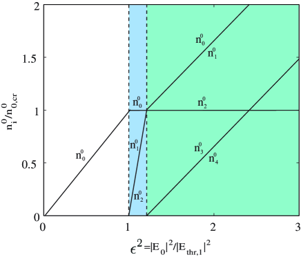
Figure 2: (Color online) Steady state solutions for the scaled intensities $n_{i}^{0}/n_{0,cr}^{0}$ of different modes ($i=0,1,...,4$) as a function of the driving field intensity parameter $\epsilon^{2}\equiv\left|E_{0}\right|^{2}/\left|E_{thr,1}\right|^{2}$, for $\gamma_{0}/\gamma=10$. Here, $n_{0,cr}^{0}=\gamma^{2}/\chi^{2}$ is the critical value of $n_{0}^{0}$ at the first threshold, $\left|E_{0}\right|^{2}=\left|E_{thr,1}\right|^{2}$ $\left(\epsilon_{thr,1}^{2}=1\right)$. The second threshold here corresponds to $\epsilon_{thr,2}^{2}=(1+\gamma/\gamma_{0})^{2}=1.21$.

III.0.1 Below threshold regime

Here, the amplitudes of all intracavity modes except the pump mode $\omega_{0}$ are zero, and we find that

$$\alpha_{1}^{0}=\alpha_{2}^{0}=\alpha_{3}^{0}=\alpha_{4}^{0}=0,$$

$$\alpha_{0}^{0}=\frac{E_{0}}{\gamma_{0}}.$$ (15)

The last equation can be rewritten in terms of the steady state intensity $n_{0}^{0}=$ $\left|\alpha_{0}^{0}\right|^{2}$ (in photon number units) and phase $\phi_{0}^{0}$ (where $\alpha_{0}^{0}=\sqrt{n_{0}^{0}}\exp(i\phi_{0}^{0})$):

$$n_{0}^{0} =\left|E_{0}\right|^{2}/\gamma_{0}^{2},\;$$

$$\phi_{0}^{0} =\varphi_{0},$$ (16)

where $\varphi_{0}$ is the phase of the driving field, i.e., $E_{0}=|E_{0}|\exp(i\varphi_{0})$. The linearized stability analysis of these steady states (see Sec. IV) reveals that they are stable for driving field intensities below a certain critical (threshold) value,

$$\left|E_{0}\right|^{2}<\left|E_{thr,1}\right|^{2},$$ (17)

where

$$\left|E_{thr,1}\right|^{2}\equiv\frac{\gamma_{0}^{2}\gamma^{2}}{\chi^{2}}$$ (18)

is the first threshold. This allows us to introduce a dimensionless relative driving field parameter,

$$\epsilon\equiv\frac{\left|E_{0}\right|}{\left|E_{thr,1}\right|}\,\,.$$

Thus, the first regime corresponds to conditions where both nonlinear crystals operate in the below threshold regime of parametric down-conversion. Here the steady state solutions for the modes $\omega_{0}$, $\omega_{1}$ and $\omega_{2}$ are the same as in the usual nondegenerate parametric down-conversion with a single crystal Reid-Drumm . Figure 2 plots the steady state solution $n_{0}^{0}$ in the below threshold regime where we have also introduced a new variable, namely $n_{0,cr}^{0}=|E_{thr,1}|^{2}/\gamma_{0}^{2}=\gamma^{2}/\chi^{2}$. This is the critical value of $n_{0}^{0}$ at the first threshold.

III.0.2 First above-threshold regime

In the first above-threshold regime, the amplitudes of the modes $\omega_{3}$ and $\omega_{4}$ remain zero, while the amplitudes of the pump, signal and idler modes ($\omega_{0}$, $\omega_{1}$ and $\omega_{2}$) are nonzero. Accordingly, we again use the intensity and phase variables, $n_{i}^{0}$ and $\phi_{i}^{0}$, $\alpha_{i}^{0}=\sqrt{n_{i}^{0}}\exp(i\phi_{i}^{0})$ for $i=0,1,2$, and write the steady state solutions as:

$$\alpha_{3}^{0} =\alpha_{4}^{0}=0,$$

$$n_{0}^{0} =\frac{\gamma^{2}}{\chi^{2}},$$

$$n_{1}^{0} =n_{2}^{0}=\frac{\left|E_{0}\right|}{\chi}-\frac{\gamma_{0}\gamma}{\chi^{2}},$$ (19)

$$\phi_{0}^{0} =\varphi_{0},$$

$$\phi_{1}^{0}+\phi_{2}^{0} =\phi_{0}^{0}=\varphi_{0}.$$ (20)

We see that the steady state intensities $n_{1}^{0}$ and $n_{2}^{0}$ correspond to physical solutions ($n_{i}^{0}>0$ ) if the driving field intensity is above the first threshold, $\left|E_{0}\right|^{2}>\left|E_{thr,1}\right|^{2}$. On the other hand, the linearized eigenvalue analysis for the sub-system of intensity variable (see below) shows that the solutions are stable for $\left|E_{0}\right|^{2}$ below a second threshold, $\left|E_{0}\right|^{2}<\left|E_{thr,2}\right|^{2}$, where

$$\left|E_{thr,2}\right|^{2}\equiv\frac{\gamma_{0}^{2}\gamma^{2}}{\chi^{2}}\left(1+\frac{\gamma}{\gamma_{0}}\right)^{2}=\left|E_{thr,1}\right|^{2}\left(1+\frac{\gamma}{\gamma_{0}}\right)^{2}.$$ (21)

This implies that the first above threshold regime is restricted to:

$$\left|E_{thr,1}\right|^{2}<\left|E_{0}\right|^{2}<\left|E_{thr,2}\right|^{2}.$$ (22)

This is shown in Fig. 2 along with the steady state solutions of Eq. (19).

In this regime, the first nonlinear crystal operates in the above-threshold (stimulated) regime, while the operation of the second nonlinear crystal is in the below-threshold (spontaneous) regime. The steady state solutions for the $\omega_{0}$, $\omega_{1}$ and $\omega_{2}$ modes are the same as in nondegenerate parametric down-conversion with a single crystal Reid-Drumm , except that the stability region has now an upper bound.

III.0.3 Second above-threshold regime

In the second above-threshold regime, both nonlinear crystals operate with stimulated emission, and the amplitudes of all intracavity modes are nonzero. The mode $\omega_{2}$ acts as the pump mode with respect to the second nonlinear crystal and its intensity is above the respective threshold for stimulated down-conversion $\omega_{2}\rightarrow\omega_{3}+\omega_{4}$. Note that $|E_{thr,2}|$ is very close to $|E_{thr,1}|$ in the case of a strongly damped or nonresonant primary pump $\hat{a}_{0}$ that we consider here. This makes this second above-threshold regime quite accessible experimentally and, in the limit $\gamma_{2}\rightarrow 0$, could bring about effective $\chi^{(3)}$ behavior (see next section).

Again using the intensity and phase variables, the steady state solutions can be written as follows:

$$n_{0}^{0}=n_{1}^{0}=\frac{\left|E_{0}\right|^{2}}{\left(\gamma_{0}+\gamma\right)^{2}},$$

$$n_{2}^{0}=\frac{\gamma^{2}}{\chi^{2}},$$

$$n_{3}^{0}=n_{4}^{0}=\frac{\left|E_{0}\right|^{2}}{\left(\gamma_{0}+\gamma\right)^{2}}-\frac{\gamma^{2}}{\chi^{2}},$$ (23)

$$\phi_{0}^{0} =\varphi_{0},$$

$$\phi_{1}^{0}+\phi_{2}^{0} =\phi_{0}^{0}=\varphi_{0},$$

$$\phi_{3}^{0}+\phi_{4}^{0}-\phi_{2}^{0} =0.$$ (24)

The intensities $n_{1}^{0}$, $n_{2}^{0}$, and $n_{3}^{0}$ ($n_{3}^{0}=n_{4}^{0}$) are related by a simple relationship

$$n_{1}^{0}=n_{2}^{0}+n_{3}^{0}.$$ (25)

This reflects the photon number conservation in the second crystal and the correlation between the photons $\omega_{1}$ and $\omega_{2}$, including the possibility of conversion of photons $\omega_{2}$ into a pair of photons $\omega_{3}$ and $\omega_{4}$. From the expressions for $n_{3}^{0}$ and $n_{4}^{0}$, we see that physical solutions are realized for driving field intensities above the second threshold,

$$\left|E_{0}\right|^{2}>\left|E_{thr,2}\right|^{2}.$$ (26)

In addition, we show in the next section that the linearized eigenvalue analysis reveals that the sub-system of intensity variables is stable in this region. Thus, the second above-threshold regime corresponds to Eq. (26) and is pictured in Fig. 2 with its corresponding steady state solutions.

IV Stability properties

Here we give the details of the linearized eigenvalue analysis to determine stability of the classical steady-state regimes. In order to explain this approach, we proceed with a dimensionless analysis, in terms of a small parameter

$$g=\frac{\chi}{\gamma}\,\,.$$ (27)

We now wish to derive the leading order behavior of the stochastic fluctuations in each mode, as an expansion in terms of $g$. It is simplest to first transform to dimensionless parameters, defining dimensionless time as:

$$\tau=\gamma t$$ (28)

This scaled time variable will be used for all derivatives defined in this section. Furthermore we will also use the dimensionless parameter

$$\gamma_{r}=\frac{\gamma_{0}}{\gamma}$$ (29)

We note here that a linearized analysis is only the first stage in a stochastic diagram perturbation expansionChaturvedi , which in general needs to be taken to higher order to reveal non-Gaussian behaviordrummond_nondeg . The details of this will be treated elsewhere.

IV.1 Positive-P method

We start by using the full positive-P method to treat this system, together with an appropriate scaling for the below threshold fields, by introducing:

$$\beta_{0} = \left(\alpha_{0}-\alpha_{0}^{0}\right)/g$$

$$\beta_{3} = \alpha_{3}/\sqrt{g}$$

$$\beta_{4} = \alpha_{4}/\sqrt{g}$$

Using the semi-classical steady state solutions, Eq. (5), and dropping higher-order terms of order $\sqrt{g}$ or higher, we get:

$$\dot{\beta}_{0} = -\gamma_{r}\beta_{0}-\alpha_{1}\alpha_{2}$$

$$\dot{\alpha}_{1} = -\alpha_{1}+\epsilon\alpha_{2}^{+}+\sqrt{\epsilon}\eta_{1}(\tau)$$

$$\dot{\alpha}_{2} = -\alpha_{2}+\epsilon\alpha_{1}^{+}+\sqrt{\epsilon}\eta_{2}(\tau)$$

$$\dot{\beta}_{3} = -\beta_{3}+\sqrt{\alpha_{2}}\eta_{3}(\tau)$$

$$\dot{\beta}_{4} = -\beta_{4}+\sqrt{\alpha_{2}}\eta_{4}(\tau)$$

together with the Hermitian conjugate equations. The nonzero steady-state correlations of the noise terms are:

$$\left\langle\eta_{1}(\tau)\eta_{2}(\tau^{\prime})\right\rangle =\delta(\tau-\tau^{\prime}),$$

$$\left\langle\eta_{3}(\tau)\eta_{4}(\tau^{\prime})\right\rangle =\delta(\tau-\tau^{\prime}),$$ (30)

The linearized equations for $\beta_{0}$ and $\beta{}_{3,4}$ are all decoupled and have negative eigenvalues $-\gamma_{0}$ and $-\gamma$, respectively. Accordingly, the corresponding steady states are stable. The deterministic part of linearized equations for the remaining variables, $\alpha_{1}$ and $\alpha_{2}$ (together with $\alpha_{1}^{+}$ and $\alpha_{2}^{+}$), can be written in the matrix form as follows:

$$\underline{\dot{\alpha}}=A^{0}\underline{\alpha},$$ (31)

where $\underline{\alpha}=\left(\alpha_{1},\alpha_{2},\alpha_{1}^{+},\alpha_{2}^{+}\right)^{T}$ and the drift matrix $A^{0}$ is given by

$$A^{0}=\left(\begin{array}[]{cccc}-1&0&0&\epsilon\\ 0&-1&\epsilon&0\\ 0&\epsilon&-1&0\\ \epsilon&0&0&-1\end{array}\right).$$ (32)

The eigenvalues of the matrix $A^{0}$ can be calculated explicitly, with the result that their real parts are all negative if

$$\epsilon^{2}<1.$$ (33)

This defines the stability region, Eq. (17), for the steady states (15) and the first threshold, Eq. (18).

IV.2 Above-threshold stability

In this section we analyze the stability of the above-threshold regimes. For reasons of length, we do not give a complete analysis of the fluctuations, but rather we simply determine which are the stable regimes. This allows us to build a complete large-signal phase-diagram, which is highly useful for determining the down-conversion properties of the cascaded device. Detailed spectral properties will be analyzed elsewhere.

IV.2.1 First above-threshold regime

Inspecting the semi-classical steady state solutions, Eqs. (19) and (20), we immediately notice that while the sum of the steady state phases $\phi_{1}^{0}+\phi_{2}^{0}$ of the signal and idler modes is well defined and is equal to the phase of the driving field, $\varphi_{0}$, the individual values of $\phi_{1}^{0}$ and $\phi_{2}^{0}$ remain unknown. In other words, there is no unique solution for the individual phases $\phi_{1}^{0}$ and $\phi_{2}^{0}$ and any attempt to perform linearization around any chosen value of $\phi_{1}^{0}$ or $\phi_{2}^{0}$ will generate a zero eigenvalue, implying that the steady states are unstable. This problem is known as phase diffusion graham-phase-diff ; Reid-Drumm .

In order to correctly analyze the set of coupled equations of motion in this regime, it is helpful to factorize them into a subset that can be linearized and is stable, while the equation associated with the zero eigenvalue must be isolated (decoupled) and treated exactly without the use of linearization. This can be achieved by means of transforming to a new set of stochastic variables. In doing so, we note that the stochastic equations of motion for this system, Eqs. (5), are equivalent in either It${\rm\hat{o}}$ or Stratonovich formulation of the stochastic calculus. We employ the Stratonovich formulation which has the advantage that the variable changes are achieved using the usual calculus rules, without any extra variable-change terms. Accordingly, we first transform to new intensity and phase variables for the modes $\omega_{0}$, $\omega_{1}$, and $\omega_{2}$:

$$n_{j}=\alpha_{j}\alpha_{j}^{+},$$

$$\phi_{j}=\frac{1}{2i}\ln\left(\frac{\alpha_{j}}{\alpha_{j}^{+}}\right),\;(j=0,1,2),$$ (34)

which we note are complex. The stochastic variables $\alpha_{3,4}$ and $\alpha_{3,4}^{+}$, on the other hand, are transformed to:

$$\widetilde{\alpha}_{3,4} =\alpha_{3,4}e^{-i\phi_{2}/2},$$

$$\widetilde{\alpha}_{3,4}^{+} =\alpha_{3,4}^{+}e^{i\phi_{2}/2}.$$ (35)

In these new variables, the stochastic differential equations become:

$$\dot{n}_{0} =-2\gamma_{0}n_{0}+2\left|E_{0}\right|\cos\left(\varphi_{0}-\phi_{0}\right)$$

$$-2\chi\sqrt{n_{0}n_{1}n_{2}}\cos\left(\phi_{0}-\phi_{+}\right),$$ (36)

$$\dot{n}_{1} =-2\gamma n_{1}+2\chi\sqrt{n_{0}n_{1}n_{2}}\cos\left(\phi_{0}-\phi_{+}\right)$$

$$+F_{1}(t),$$ (37)

$$\dot{n}_{2} =-2\gamma n_{2}+2\chi\sqrt{n_{0}n_{1}n_{2}}\cos\left(\phi_{0}-\phi_{+}\right)$$

$$-\chi\sqrt{n_{2}}\left(\widetilde{\alpha}_{3}\widetilde{\alpha}_{4}+\widetilde{\alpha}_{3}^{+}\widetilde{\alpha}_{4}^{+}\right)+F_{2}(t),$$ (38)

$$\dot{\phi}_{0} =\frac{\left|E_{0}\right|}{n_{0}}\sin\left(\phi_{0}-\phi_{+}\right)$$

$$\,\,\,\,-\chi\sqrt{\frac{n_{1}n_{2}}{n_{0}}}\sin\left(\phi_{0}-\phi_{+}\right),$$ (39)

$$\dot{\phi}_{1} =\chi\sqrt{\frac{n_{0}n_{2}}{n_{1}}}\sin\left(\phi_{0}-\phi_{+}\right)+f_{1}(t),$$ (40)

$$\dot{\phi}_{2} =\chi\sqrt{\frac{n_{0}n_{1}}{n_{2}}}\sin\left(\phi_{0}-\phi_{+}\right)$$

$$-\frac{\chi}{2i\sqrt{n_{2}}}\left(\widetilde{\alpha}_{3}\widetilde{\alpha}_{4}-\widetilde{\alpha}_{3}^{+}\widetilde{\alpha}_{4}^{+}\right)+f_{2}(t),$$ (41)

$$\dot{\widetilde{\alpha}}_{3} =-\gamma\widetilde{\alpha}_{3}+\chi\sqrt{n_{2}}\widetilde{\alpha}_{4}^{+}-\frac{i\chi}{2}\sqrt{\frac{n_{0}n_{1}}{n_{2}}}\widetilde{\alpha}_{3}\sin\left(\phi_{0}-\phi_{+}\right)$$

$$+\frac{\chi}{4\sqrt{n_{2}}}\left(\widetilde{\alpha}_{3}\widetilde{\alpha}_{4}-\widetilde{\alpha}_{3}^{+}\widetilde{\alpha}_{4}^{+}\right)\widetilde{\alpha}_{3}+\mathcal{F}_{3}(t),$$ (42)

$$\dot{\widetilde{\alpha}}_{4} =-\gamma\widetilde{\alpha}_{4}+\chi\sqrt{n_{2}}\widetilde{\alpha}_{3}^{+}-\frac{i\chi}{2}\sqrt{\frac{n_{0}n_{1}}{n_{2}}}\widetilde{\alpha}_{4}\sin\left(\phi_{0}-\phi_{+}\right)$$

$$+\frac{\chi}{4\sqrt{n_{2}}}\left(\widetilde{\alpha}_{3}\widetilde{\alpha}_{4}-\widetilde{\alpha}_{3}^{+}\widetilde{\alpha}_{4}^{+}\right)\widetilde{\alpha}_{4}+\mathcal{F}_{4}(t).$$ (43)

together with the equations for $\widetilde{\alpha}_{3}^{+}$ and $\widetilde{\alpha}_{4}^{+}$. Here, we have defined the sum of the phase variables $\phi_{1}$ and $\phi_{2}$ via

$$\phi_{+}\equiv\phi_{1}+\phi_{2},$$ (44)

and we note that the equations for $\widetilde{\alpha}_{3}$ and $\widetilde{\alpha}_{4}$ contain terms that come from the time derivative of $\phi_{2}$ which have been substituted with the right-hand side of Eq. (41).

The new noise terms in the above set of equations of motion are defined according to:

$$F_{1,2} =\alpha_{1,2}^{+}\sqrt{\chi\alpha_{0}}\zeta_{1,2}+\alpha_{1,2}\sqrt{\chi\alpha_{0}^{+}}\zeta_{1,2}^{+},$$ (45)

$$f_{1,2} =\frac{\sqrt{\chi\alpha_{0}}}{2i\alpha_{1,2}}\zeta_{1,2}-\frac{\sqrt{\chi\alpha_{0}^{+}}}{2i\alpha_{1,2}^{+}}\zeta_{1,2}^{+},$$ (46)

$$\mathcal{F}_{3,4} =\sqrt{\chi\alpha_{2}}e^{-i\phi_{2}/2}\zeta_{3,4}-\frac{i\widetilde{\alpha}_{3,4}}{2}f_{2}.$$ (47)

These must be rewritten in terms of the intensity and phase variables $n_{i}$ and $\phi_{i}$, for self-consistency:

$$F_{1,2} =\sqrt{\chi n_{1,2}}(n_{0})^{1/4}\left[e^{-i\phi_{1,2}+i\phi_{0}/2}\zeta_{1,2}\right.$$

$$\left.+e^{i\phi_{1,2}-i\phi_{0}/2}\zeta_{1,2}^{+}\right],$$ (48)

$$f_{1,2} =\frac{\sqrt{\chi}(n_{0})^{1/4}}{2i\sqrt{n_{1,2}}}\left[e^{-i\phi_{1,2}+i\phi_{0}/2}\zeta_{1,2}\right.$$

$$\left.-e^{i\phi_{1,2}-i\phi_{0}/2}\zeta_{1,2}^{+}\right],$$ (49)

$$\mathcal{F}_{3,4}=\sqrt{\chi}(n_{2})^{1/4}\zeta_{3,4}-\frac{i\widetilde{\alpha}_{3,4}}{2}f_{2}.\;$$ (50)

We next introduce the phase sum and difference variables,

$$\phi_{\pm}=\phi_{1}\pm\phi_{2},$$ (51)

and convert the equations of motion for $\phi_{1}$ and $\phi_{2}$ into:

$$\dot{\phi}_{+} =\chi\sqrt{n_{0}}\left(\sqrt{\frac{n_{2}}{n_{1}}}+\sqrt{\frac{n_{1}}{n_{2}}}\right)\sin\left(\phi_{0}-\phi_{+}\right)$$

$$-\frac{\chi}{2i\sqrt{n_{2}}}\left(\widetilde{\alpha}_{3}\widetilde{\alpha}_{4}-\widetilde{\alpha}_{3}^{+}\widetilde{\alpha}_{4}^{+}\right)+f_{+}(t),$$ (52)

$$\dot{\phi}_{-} =\chi\sqrt{n_{0}}\left(\sqrt{\frac{n_{2}}{n_{1}}}-\sqrt{\frac{n_{1}}{n_{2}}}\right)\sin\left(\phi_{0}-\phi_{+}\right)$$

$$+\frac{\chi}{2i\sqrt{n_{2}}}\left(\widetilde{\alpha}_{3}\widetilde{\alpha}_{4}-\widetilde{\alpha}_{3}^{+}\widetilde{\alpha}_{4}^{+}\right)+f_{-}(t),$$ (53)

where the noise terms are

$$f_{\pm}=f_{1}\pm f_{2}.$$ (54)

We now immediately see, that the equations of motion for the variables $n_{0}$, $n_{1}$, $n_{2}$, $\widetilde{\alpha}_{3,4}$, $\widetilde{\alpha}_{3,4}^{+}$, $\phi_{0}$ and $\phi_{+}$ are decoupled from the equation of motion for the phase-difference variable $\phi_{-}$. All these variables except $\phi_{-}$ have a unique semi-classical steady state solution given by Eqs. (19)-(20), with $\phi_{+}^{0}=\phi_{1}^{0}+\phi_{2}^{0}=\varphi_{0}$ and $\widetilde{\alpha}_{3,4}^{0}=0$ (along with $(\widetilde{\alpha}_{3,4}^{0})^{+}=(\widetilde{\alpha}_{3,4}^{0})^{\ast}=0$). As we will show below, the linearized equations for this subsystem of variables are stable, and therefore these variables can be treated by means of linearization around their semi-classical steady states. Indeed, by introducing small fluctuations around the steady states

$$\delta n_{0,1,2}(t) =n_{0,1,2}(t)-n_{0,1,2}^{0},$$ (55)

$$\delta\widetilde{\alpha}_{3,4}(t) =\widetilde{\alpha}_{3,4}(t)-\widetilde{\alpha}_{3,4}^{0},$$ (56)

$$\delta\widetilde{\alpha}_{3,4}^{+}(t) =\widetilde{\alpha}_{3,4}^{+}(t)-(\widetilde{\alpha}_{3,4}^{0})^{\ast},$$ (57)

$$\delta\phi_{0,+}(t) =\phi_{0,+}(t)-\phi_{0,+}^{0},$$ (58)

we obtain the following set of linearized equations:

$$\delta\dot{n}_{0}=-\gamma_{0}\delta n_{0}-\gamma\delta n_{+},$$ (59)

$$\delta\dot{n}_{+}=\frac{2\chi n_{1}^{0}}{\gamma}\delta n_{0}+F_{+}^{0}(t),$$ (60)

$$\delta\dot{n}_{-}=-2\gamma\delta n_{-}+F_{-}^{0}(t),$$ (61)

$$\delta\dot{\phi}_{0}=-\gamma_{0}\delta\phi_{0}-\frac{\chi^{2}n_{1}^{0}}{\gamma}\delta\phi_{+},$$ (62)

$$\delta\dot{\phi}_{+}=-2\chi\delta\phi_{+}+2\gamma\delta\phi_{0}+f_{+}^{0}(t),$$ (63)

$$\delta\dot{\widetilde{\alpha}}_{3} =-\gamma\delta\widetilde{\alpha}_{3}+\chi\sqrt{n_{1}^{0}}\delta\widetilde{\alpha}_{4}^{+}+\mathcal{F}_{3}^{0}(t),$$ (64)

$$\delta\dot{\widetilde{\alpha}}_{4} =-\gamma\delta\widetilde{\alpha}_{4}+\chi\sqrt{n_{1}^{0}}\delta\widetilde{\alpha}_{3}^{+}+\mathcal{F}_{4}^{0}(t),$$ (65)

together with the equations for $\delta\widetilde{\alpha}_{3,4}^{+}$. Here, we have used the explicit expression for the steady state solution $n_{0}^{0}$ from Eq. (19) and the fact that $n_{1}^{0}=n_{2}^{0}$. The nonzero steady-state correlations of the noise terms, in the small-noise approximation, are given by:

$$\left\langle F_{+}^{0}(t)F_{+}^{0}(t^{\prime})\right\rangle =-\left\langle F_{-}^{0}(t)F_{-}^{0}(t^{\prime})\right\rangle$$

$$=4\gamma n_{1}^{0}\delta(t-t^{\prime}),$$ (66)

$$\left\langle f_{+}^{0}(t)f_{+}^{0}(t^{\prime})\right\rangle =-\frac{\gamma}{n_{1}^{0}}\delta(t-t^{\prime}),$$ (67)

$$\left\langle\mathcal{F}_{3}^{0}(t)\mathcal{F}_{4}^{0}(t^{\prime})\right\rangle =\chi\sqrt{n_{1}^{0}}\delta(t-t^{\prime}),$$ (68)

By substituting the steady state intensity $n_{1}^{0}$ from Eqs. (19), the linearized equations and hence their solutions can be expressed in terms of the driving field intensity $\left|E_{0}\right|^{2}$.

The eigenvalue analysis of the deterministic drift terms of the linearized equations reveals that the equations for $\delta n_{0,+}$, $\delta n_{-}$, and $\delta\phi_{0,+}$ are stable everywhere (the eigenvalues have negative real parts), while the subsystem of variables $\left(\delta\widetilde{\alpha}_{3},\delta\widetilde{\alpha}_{4},\delta\widetilde{\alpha}_{3}^{+},\delta\widetilde{\alpha}_{4}^{+}\right)$ is stable only if

$$\left|E_{0}\right|^{2}<\frac{\gamma_{0}^{2}\gamma^{2}}{\chi^{2}}\left(1+\frac{\gamma}{\gamma_{0}}\right)^{2}.$$ (69)

This defines the second threshold, Eq. (21), and hence the upper bound on the driving field intensity $\left|E_{0}\right|^{2}$ for the first above-threshold region, Eq. (22).

The remaining equation for the phase difference variable $\phi_{-}$, Eq. (53), can not be linearized since the steady state solution is not well defined and linearization around any chosen value $\phi_{-}^{0}$ will reveal a zero eigenvalue, implying that the equation is not stable. The right hand side of Eq. (53) can, however, be simplified since all variables here can be linearized around their stable steady states. Thus, expanding these in terms of the stable steady states plus small fluctuations and keeping only the linear terms, we see that the deterministic terms all cancel each other. The resulting equation is

$$\dot{\phi}_{-}=f_{-}^{0}(t),$$ (70)

with the following nonzero correlation of the noise term:

$$\left\langle f_{-}^{0}(t)f_{-}^{0}(t^{\prime})\right\rangle=\frac{\gamma}{n_{1}^{0}}\delta(t-t^{\prime}).$$ (71)

Thus, we have isolated the instability associated with a zero eigenvalue into a single phase variable, which is the phase difference $\phi_{-}$ between the signal and idler phases. Unlike the other variables, the phase difference $\phi_{-}$ is not a small fluctuation around a stable steady state. Instead it undergoes continuous phase diffusion, governed by the noise term $f_{-}^{0}(t)$ in Eq. (70).

Despite the fact that the noise terms $F_{1,2}$ and $f_{1,2}$ (and hence $F_{+,-}\,\,$and$\,\,f_{+,-}$) depend explicitly on the individual phases of the signal and idler modes, (which are not well-defined), nevertheless, upon calculating the steady state noise correlations, Eqs. (66) - (68), these phases combine into the phase sum $\phi_{+}=\phi_{1}+$ $\phi_{2}$ which has a well defined steady state value and is stable. As a result, calculation of observables via the solutions of the linearized equations of motion, Eqs. (59 ) - (65) which ultimately depend on the noise correlations – is a well defined procedure, and is independent on the individual phases $\phi_{1}$ and $\phi_{2}$ .

IV.3 Second above-threshold regime

In the second above threshold regime, both parametric down-converters operate in the above-threshold regime. In addition to the phase diffusion in the signal and idler modes $\omega_{1}$ and $\omega_{2}$, we now have a second source of instability which comes from the phase diffusion in the secondary signal-idler modes, $\omega_{3}$ and $\omega_{4}$. To simplify our analysis, we assume here that the damping constant of the pump mode $\gamma_{0}$ is much larger than the damping constants of all the other modes,

$$\gamma_{0}\gg\gamma.$$ (72)

Under this condition, one can adiabatically eliminate the pump mode from the equations of motion, Eq. (5), and restrict ourselves to the dynamics of the remaining modes $\omega_{1}$, $\omega_{2}$, $\omega_{3}$, and $\omega_{4}$. Thus, we assume that $\dot{\alpha}_{0}=0$ during the evolution of the amplitudes $\alpha_{1,2,3,4}$, and we use the resulting expression for $\alpha_{0}$,

$$\alpha_{0}=\frac{1}{\gamma_{0}}\left(E_{0}-\chi\alpha_{1}\alpha_{2}\right),$$ (73)

(together with the expression for $\alpha_{0}^{+}$) in the equations for $\alpha_{1,2,3,4}$. Transforming then to the intensity and phase variables, as in Eq. (34), we obtain the following set of stochastic equations for the intensities:

$$\dot{n}_{1} =-2\gamma n_{1}+\frac{2\chi\left|E_{0}\right|}{\gamma_{0}}\sqrt{n_{1}n_{2}}\cos\theta_{1}-\frac{2\chi^{2}}{\gamma_{0}}n_{1}n_{2}$$

$$+F_{1}(t),$$ (74)

$$\dot{n}_{2} =-2\gamma n_{2}\,+\frac{2\chi\left|E_{0}\right|}{\gamma_{0}}\sqrt{n_{1}n_{2}}\cos\theta_{1}-\frac{2\chi^{2}}{\gamma_{0}}n_{1}n_{2}$$

$$-2\chi\sqrt{n_{2}n_{3}n_{4}}\cos\theta_{2}+F_{2}(t),$$ (75)

$$\dot{n}_{3} =-2\gamma n_{3}+2\chi\sqrt{n_{2}n_{3}n_{4}}\cos\theta_{2}+F_{3}(t),$$ (76)

$$\dot{n}_{4} =-2\gamma n_{4}+2\chi\sqrt{n_{2}n_{3}n_{4}}\cos\theta_{2}+F_{4}(t),$$ (77)

Here, we have defined

$$\theta_{1} =\phi_{1}+\phi_{2}-\varphi_{0},$$ (78)

$$\theta_{2} =\phi_{3}+\phi_{4}-\phi_{2}.$$ (79)

which can serve as a new pair of phase variables, traded in favor of the the signal and idler phases $\phi_{1}$ and $\phi_{2}$.

The stochastic equations of motion for the phase variables, which we write at once in terms of $\theta_{1}$, $\theta_{2}$, $\phi_{3}$ and $\phi_{4}$, are:

$$\dot{\theta}_{1} =-\frac{\chi\left|E_{0}\right|}{\gamma_{0}}\left(\sqrt{\frac{n_{1}}{n_{2}}}+\sqrt{\frac{n_{2}}{n_{1}}}\right)\sin\theta_{1}$$

$$-\chi\sqrt{\frac{n_{3}n_{4}}{n_{2}}}\sin\theta_{2}+f_{\theta_{1}}(t),$$ (80)

$$\dot{\theta}_{2} =-\chi\left(\sqrt{\frac{n_{2}n_{3}}{n_{4}}}+\sqrt{\frac{n_{2}n_{4}}{n_{3}}}-\sqrt{\frac{n_{3}n_{4}}{n_{2}}}\right)\sin\theta_{2}$$

$$+\frac{\chi\left|E_{0}\right|}{\gamma_{0}}\sqrt{\frac{n_{1}}{n_{2}}}\sin\theta_{1}+f_{\theta_{2}}(t),$$ (81)

$$\dot{\phi}_{3} =-\chi\sqrt{\frac{n_{2}n_{4}}{n_{3}}}\sin\theta_{2}+f_{3}(t),$$ (82)

$$\dot{\phi}_{4} =-\chi\sqrt{\frac{n_{2}n_{3}}{n_{4}}}\sin\theta_{2}+f_{4}(t).$$ (83)

In the above equations, the noise terms are given by

$$f_{\theta_{1}} =f_{1}+f_{2},$$ (84)

$$f_{\theta_{2}} =f_{3}+f_{4}-f_{2},$$ (85)

and

$$f_{1,2} =\frac{1}{2i\alpha_{1,2}}\sqrt{\frac{\chi}{\gamma_{0}}(E_{0}-\chi\alpha_{1}\alpha_{2})}\zeta_{1,2}$$

$$-\frac{1}{2i\alpha_{j}^{+}}\sqrt{\frac{\chi}{\gamma_{0}}(E_{0}^{\ast}-\chi\alpha_{1}^{+}\alpha_{2}^{+})}\zeta_{1,2}^{+},$$ (86)

$$f_{3,4} =\frac{\sqrt{\chi\alpha_{2}}}{2i\alpha_{3,4}}\zeta_{3,4}-\frac{\sqrt{\chi\alpha_{2}^{+}}}{2i\alpha_{3,4}^{+}}\zeta_{3,4}^{+}.$$ (87)

In addition, the noise terms $F_{1,2,3,4}$ in Eqs. (74 )-(77) are given by

$$F_{1,2}(t) =\alpha_{1,2}^{+}\sqrt{\frac{\chi}{\gamma_{0}}(E_{0}-\chi\alpha_{1}\alpha_{2})}\zeta_{1,2}\,$$

$$+\alpha_{1,2}\sqrt{\frac{\chi}{\gamma_{0}}(E_{0}^{\ast}-\chi\alpha_{1}^{+}\alpha_{2}^{+})}\zeta_{1,2}^{+},$$ (88)

$$F_{3,4}(t) =\alpha_{3,4}^{+}\sqrt{\chi\alpha_{2}}\zeta_{3,4}+\alpha_{3,4}\sqrt{\chi\alpha_{2}^{+}}\zeta_{3,4}^{+}.$$ (89)

In all these noise terms the amplitude variables have to be expressed in terms of the intensity and phase variables for self-consistency.

By inspecting Eqs. (74)-(77) and Eqs. (80)-(83), we see that the equations for the intensities $n_{1,2,3,4}$ and phases $\theta_{1,2}$ are decoupled from the equations for the phase variables, $\phi_{3,4}$. The variables $n_{1,2,3,4}$ and $\theta_{1,2}$ all have well defined semi-classical steady states, c.f., Eqs. (23) and (24), with $\theta_{1,2}^{0}=0$, and as we will show below, the linearized eigenvalue analysis indicates their stability. Thus, this subsystem of variables can be treated within the linearized treatment of fluctuations. The phase variables $\phi_{3}$ and $\phi_{4}$, on the other hand, do not have stable semi-classical steady states and can not be treated by means of linearization. To demonstrate the stability of the intensities $n_{1,2,3,4}$ and phases $\theta_{1,2}$, we introduce fluctuations around the semi-classical steady states,

$$\delta n_{j}(t) =n_{j}(t)-n_{j}^{0},\;(j=1,2,3,4),$$ (90)

$$\delta\theta_{1,2}(t) =\theta_{1,2}(t)-\theta_{1,2}^{0},$$ (91)

and derive the following linearized equations for the intensity fluctuations:

$$\dot{\delta n}_{1} =-\gamma\left(1+\frac{\gamma}{\gamma_{0}}\right)\delta n_{1}$$

$$+\frac{\chi^{2}n_{1}^{0}}{\gamma}\left(1-\frac{\gamma}{\gamma_{0}}\right)\delta n_{2}+F_{1}^{0}(t),$$ (92)

$$\dot{\delta n_{2}} =-\gamma\left(1+\frac{\chi^{2}}{\gamma_{0}\gamma}\right)\delta n_{2}$$

$$+\gamma\left(1-\frac{\gamma}{\gamma_{0}}\right)\delta n_{1}-\gamma\delta n_{+}+F_{2}^{0}(t),$$ (93)

$$\dot{\delta n_{+}} =\frac{2\chi^{2}n_{3}^{0}}{\gamma}\delta n_{2}+F_{+}^{0}(t),$$ (94)

$$\dot{\delta n_{-}} =-2\gamma\delta n_{-}+F_{-}^{0}(t),$$ (95)

where we have additionally transformed to the intensity sum and difference variables

$$\delta n_{+}=\delta n_{3}+\delta n_{4},$$

$$\delta n_{-}=\delta n_{3}-\delta n_{4},$$ (96)

to further simplify the eigenvalue analysis. We have also defined

$$F_{\pm}^{0}\equiv F_{3}^{0}\pm F_{4}^{0}.$$ (97)

As we see, the equation for the intensity difference $\delta n_{-}$ fluctuation is decoupled and immediately results in a negative eigenvalue in the drift term, implying stability. The coupled equations for fluctuations in $\delta n_{1}$, $\delta n_{2}$, and $\delta n_{+}$ result in a cubic equation for the eigenvalues of the respective drift matrix. While this cannot be solved explicitly, however, the negative real parts of the eigenvalues required for stability is ascertained here using the Routh-Hurwitz criterion mathhandbook .

The linearized equations for the phase fluctuations $\delta\theta_{1,2}(t)$ are:

$$\dot{\delta\theta_{1}} =-\frac{\chi\left|E_{0}\right|}{\gamma_{0}}\left(\sqrt{\frac{n_{1}^{0}}{n_{2}^{0}}}+\sqrt{\frac{n_{2}^{0}}{n_{1}^{0}}}\right)\delta\theta_{1}$$

$$-\chi\frac{n_{3}^{0}}{\sqrt{n_{2}^{0}}}\delta\theta_{2}+f_{\theta_{1}}^{0},$$ (98)

$$\dot{\delta\theta_{2}} =-\chi\left(2\sqrt{n_{2}^{0}}-\frac{n_{3}^{0}}{\sqrt{n_{2}^{0}}}\right)\delta\theta_{2}$$

$$\,\,\,\,+\frac{\chi\left|E_{0}\right|}{\gamma_{0}}\sqrt{\frac{n_{1}^{0}}{n_{2}^{0}}}\delta\theta_{1}+f_{\theta_{2}}^{0},$$ (99)

The eigenvalues of the corresponding drift matrix can be found explicitly, with the result that they all have negative real parts and therefore the equations are stable. The nonzero steady state correlations of the noise terms in the linearized Eqs. (92)-(95) and Eqs. (98)-(99) are:

$$\left\langle F_{1}^{0}(t)F_{2}^{0}(t^{\prime})\right\rangle =2\gamma n_{1}^{0}\delta(t-t^{\prime}),$$ (100)

$$\left\langle F_{+}^{0}(t)F_{+}^{0}(t^{\prime})\right\rangle =-\left\langle F_{-}^{0}(t)F_{-}^{0}(t^{\prime})\right\rangle$$

$$=-2\left\langle F_{3}^{0}(t)F_{4}^{0}(t^{\prime})\right\rangle$$

$$=4\gamma n_{3}^{0}\delta(t-t^{\prime}),$$ (101)

$$\left\langle f_{\theta_{1}}^{0}(t)f_{\theta_{1}}^{0}(t^{\prime})\right\rangle =-2\left\langle f_{\theta_{1}}^{0}(t)f_{\theta_{2}}^{0}(t^{\prime})\right\rangle$$

$$=2\left\langle f_{1}^{0}(t)f_{2}^{0}(t^{\prime})\right\rangle$$

$$=-\frac{\chi^{2}}{\gamma}\delta(t-t^{\prime}),$$ (102)

$$\left\langle f_{\theta_{2}}^{0}(t)f_{\theta_{2}}^{0}(t^{\prime})\right\rangle =2\left\langle f_{3}^{0}(t)f_{4}^{0}(t^{\prime})\right\rangle$$

$$=-\frac{\gamma}{n_{3}^{0}}\delta(t-t^{\prime}).$$ (103)

The remaining phase variables, $\phi_{3}$ and $\phi_{4}$, cannot be treated within the linearized fluctuation treatment, however, the right hand sides of the corresponding equations of motion, Eqs. (82) and (83 ), can be simplified since all variables here have stable steady states and can be linearized. This gives

$$\dot{\phi_{3}} =-\gamma\delta\theta_{2}+f_{3}^{0}(t),$$ (104)

$$\dot{\phi_{4}} =-\gamma\delta\theta_{2}+f_{4}^{0}(t).$$ (105)

where the nonzero steady state correlation of the noise terms is given in Eq. (103). To further simplify the analysis we introduce the sum and difference phase variables

$$\theta_{\pm}=\phi_{3}\pm\phi_{4},$$ (106)

for which the equations of motions are

$$\dot{\theta}_{+} =-2\gamma\delta\theta_{2}+f_{\theta_{+}}^{0}(t),$$ (107)

$$\dot{\theta}_{-} =f_{\theta_{-}}^{0}(t),$$ (108)

The source of instability for the phase variable $\theta_{-}$ is obvious, while for the phase variable $\theta_{+}$ the presence of a zero eigenvalue is revealed when the corresponding linearized equation is combined with Eqs. (98)-(99). Thus the variables $\theta_{+}$ and $\theta_{-}$ can not be linearized, and have to be treated exactly. The nonzero correlations of the noise terms $f_{\theta_{+}}^{0}=f_{3}^{0}+f_{4}^{0}$ and $f_{\theta_{-}}^{0}=f_{3}^{0}-f_{4}^{0}$ are

$$\left\langle f_{\theta_{+}}^{0}(t)f_{\theta_{+}}^{0}(t^{\prime})\right\rangle =-\left\langle f_{\theta_{-}}^{0}(t)f_{\theta_{-}}^{0}(t^{\prime})\right\rangle$$

$$=2\left\langle f_{3}^{0}(t)f_{4}^{0}(t^{\prime})\right\rangle$$

$$=-\frac{\gamma}{n_{3}^{0}}\delta(t-t^{\prime}).$$ (109)

From Eq. (107) we see that the dynamics of the phase variable $\theta_{+}$ depends on phase fluctuations in $\delta\theta_{2}$, and therefore the equation for $\theta_{+}$ has to be integrated after solving for $\delta\theta_{2}$, Eqs. (98 )-(99). The solution for $\theta_{+}(t)$ can be written as

$$\theta_{+}(t)=\theta_{+}(t_{0})+\int_{t_{0}}^{t}\left[-2\gamma\delta\theta_{2}(t^{\prime})+f_{\theta_{+}}^{0}(t^{\prime})\right]dt^{\prime},$$ (110)

while the solution for $\theta_{-}(t)$ is

$$\theta_{-}(t)=\theta_{-}(t_{0})+\int_{t_{0}}^{t}f_{\theta_{-}}^{0}(t^{\prime})dt^{\prime}.$$ (111)

Since $\delta\theta_{2}(t)$ as a solution to the set of linearized Eqs. (98)-(99) depends on the noise terms $f_{\theta_{1}}^{0}$ and $f_{\theta_{2}}^{0}$, the calculation of correlations involving the phase sum variable $\theta_{+}(t)$ will also depend on the following nonzero noise correlation:

$$\left\langle f_{\theta_{+}}^{0}(t)f_{\theta_{2}}^{0}(t^{\prime})\right\rangle=2\left\langle f_{3}^{0}(t)f_{4}^{0}(t^{\prime})\right\rangle=-\frac{\gamma}{n_{3}^{0}}\delta(t-t^{\prime}),$$ (112)

while $\left\langle f_{\theta_{+}}^{0}(t)f_{\theta_{1}}^{0}(t^{\prime})\right\rangle=0$.

This completes the analysis of the system in the second above-threshold regime.

V Numerical simulations

A qualitative reasoning identifies the far-above-second-threshold situation as interesting for mimicking a $\chi^{(3)}$ OPO, in the regime where losses for the intermediate pump $\hat{a}_{2}$ are negligible, i.e., $\gamma_{2}\ll\gamma_{1}=\gamma_{3}=\gamma_{4}\ll\gamma_{0}$ (note that this is different to the condition given in Eq. (13)). Indeed, these hypotheses should yield close-to-ideal down-conversion rate from field $\hat{a}_{2}$ to signal fields $\hat{a}_{3}$ and $\hat{a}_{4}$, comparable to the emission rate into $\hat{a}_{1}$, and therefore be consistent with the expectation of threefold quantum correlations between $\hat{a}_{1}$, $\hat{a}_{3}$, $\hat{a}_{4}$, which should be non-Gaussian (another favorable situation for this effect would be the case $\chi_{2}\gg\chi_{1}$). The goal of the following numerical simulations is therefore to ascertain the stability of the resonant cascade in such cases, which are not covered by the previous analytical treatment.

The numerical treatment is limited to the classical equations of motion, given by Eq. (5) with $\zeta_{i}=0,i\in[0,4]$, which are integrated numerically using a fourth order Runge-Kutta routine similar to the method given in lugiato . The first and second nonlinearities were taken to be equal, i.e., $\chi_{1}=\chi_{2}$. All down-converted fields were given minute initial amplitudes and random initial phases, of which the subsequent dynamical phases were independent.

Figure 3: OPO intracavity powers for $\gamma_{2}=0.08,\gamma_{1,3,4}=0.14,\gamma_{0}=2.0,|E_{0}|/|E_{thresh,2}|=3.5$, for zero detunings.

Figure 4: Individual field phases, going through the second threshold, for $\gamma_{2}=0.08,\gamma_{1,3,4}=0.14,\gamma_{3}=1.0,|E_{0}|/|E_{thresh,2}|=3.5$, for zero detunings.

Figure 5: The phase differences $\theta_{1}$ and $\theta_{2}$ between the fields involved in the first and second stages of the nondegenerate interaction, going through the second threshold, for $\gamma_{2}=0.08,\gamma_{1,3,4}=0.14,\gamma_{3}=1.0,|E_{0}|/|E_{thresh,2}|=3.5$, for zero detunings. The stationary phase differences above the second threshold indicate that down-conversion is taking place in both stages.

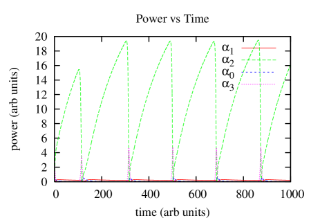
Figure 6: OPO intracavity powers for $\gamma_{2}=0.001,\gamma_{1,3,4}=0.14,\gamma_{0}=1.0,|E_{0}|/|E_{thresh,2}|=5.8$, for zero detunings. Note that $\alpha_{4}$ is omitted since its plot follows exactly $\alpha_{3}$. The spiking frequency increases with $|E_{0}|/|E_{thresh,2}|$ when other parameters are held constant.

Figure 7: Top: OPO intracavity powers for $(\gamma_{0},\gamma_{2},\gamma_{1})=(10,0,0.02)$, $|E_{0}|/|E_{thresh,2}|=0.7$. Bottom: Phase differences $\theta_{1}$ and $\theta_{2}$, for the same conditions (phases are numerically wrapped inside $[-\pi,\pi]$).

Figure 8: Phase differences $\theta_{1}$ and $\theta_{2}$, for zero detunings and $|E_{0}|/|E_{thresh,2}|=2.0$. Top: $\gamma_{2}=0.08$, $\gamma_{1}=0.14$. Bottom: $\gamma_{1}=\gamma_{2}=0.14$ (phases are numerically wrapped inside $[-\pi,\pi]$).

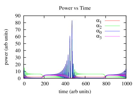
Figure 9: OPO intracavity powers for $\gamma_{0}=0.08,\gamma_{1,3,4}=0.14,|E_{0}|/|E_{thresh,2}|=2.8$, for zero detunings. Top: $\gamma_{2}=0.09$. Bottom: $\gamma_{2}=0.14$.

V.1 Steady-state solutions

As mentioned above, we restrict our analysis to a set of parameters such that $\gamma_{2}\ll\gamma_{1}=\gamma_{3}=\gamma_{4}\ll\gamma_{0}$. That is, the primary pump mode is not resonant, the intermediate pump is highly resonant (most of its losses occur in down-conversion), and the signal fields are sufficiently resonant to acquire a threshold as low as a typical single-stage, doubly resonant OPO (DRO). In this case the OPO fields show decaying oscillations to a steady state after reaching the second threshold. Higher losses for $\gamma_{2}$ result in over-damping. Figure 3 illustrates the steady-state solutions. Both thresholds are clearly visible. At long times ($t>100$ in Fig. 3) the field amplitudes match the stationary solutions of the previous section. Increasing $E_{0}$ or $\gamma_{2}$ causes the oscillations to decay more quickly.

Figure 4 shows the individual phases as the second threshold is reached. The final phase in the steady state is independent of the initial starting phase of any of the fields’ seed values. (The primary pump parameter $E_{0}$ is taken to be real.) Figure 5 shows the nonlinear phase differences $\theta_{1}$ and $\theta_{2}$ for the first and second stages of the OPO. It is clear from these phase differences that the system is in a state of cascaded parametric down-conversion.

Figure 10: Evolution of intracavity fields for $\gamma_{0}=1.0,\gamma_{2}=0.08,\gamma_{1,3,4}=0.14,|E_{0}|/|E_{thresh,2}|=3.5$, perturbation $\delta_{\alpha i}=\alpha_{i}$, for zero detunings. The perturbation has been applied simultaneously to the real and imaginary parts of the fields, leaving no net perturbation to the phases.

Figure 11: Evolution of the phase differences $\theta_{1}$ and $\theta_{2}$ for $\gamma_{0}=1.0,\gamma_{2}=0.08,\gamma_{1,3,4}=0.14,|E_{0}|/|E_{thresh,2}|=3.5$, perturbation $\delta_{\alpha i}=\alpha_{i}$, for zero detunings. The perturbation has been applied to the imaginary parts of the fields.

Figure 12: Evolution of intracavity fields for $\gamma_{0}=1.0,\gamma_{2}=0.08,\gamma_{1,3,4}=0.14,|E_{0}|/|E_{thresh,2}|=3.5$, perturbation $\delta_{\alpha i}=\alpha_{i}$, for zero detunings. The perturbation has been applied to the real part of the field amplitudes.

Figure 13: Evolution of the OPO phases for $\gamma_{0}=1.0,\gamma_{2}=0.08,\gamma_{1,3,4}=0.14,|E_{0}|/|E_{thresh,2}|=3.5$, perturbation $\delta_{\alpha i}=\alpha_{i}$, for zero detunings. The perturbation has been applied to the real part of the fields. Top: individual phases. Bottom: $\theta_{1}$ and $\theta_{2}$ (phases are numerically wrapped inside $[-\pi,\pi]$).

V.2 Second above-threshold regime for low $\gamma_{2}$

V.2.1 Nondegenerate cascade

One interesting question is that of obtaining a stable effective $\chi^{(3)}$ OPO by lowering $\gamma_{2}$ and operating well above second threshold. In that case, the nondegenerate and degenerate cascades do not exhibit the same behavior. As the intermediate pump loss rate is lowered, a spiking instability is obtained in both cases, as displayed in Fig. 6 for the nondegenerate case. One may overcome this self-pulsing and induce a transition to a stable steady state by increasing the pump parameter above threshold. The lower $\gamma_{2}$ the higher $|E_{0}|/|E_{thresh,2}|$ needs to be to achieve steady state in the nondegenerate case.

V.2.2 Degenerate cascade

In the degenerate case, a remarkable result is that the spiking behavior is always transient and relaxes into a stationary state. However, more insight into the behavior of the degenerate cascade is obtained, once again, by scrutinizing the evolution of the phases $\theta_{1}$ and $\theta_{2}$. This bears particular physical significance for the degenerate cascade because the first stage can stimulate emission in the second stage, which cannot happen in the nondegenerate cascade due to the indistinguishability of the signal fields note . Because of this effect, the degenerate cascade will exhibit greater sensitivity to the evolution of $\theta_{1}$ and $\theta_{2}$, whose swings translate into the appearance of competing sum-frequency generation (SFG) processes in both stages.

First above-threshold:

Figure 7 (top) displays the damping of the low $\gamma_{2}$ spiking. The phase behavior is plotted in Fig. 7 (bottom) and shows that significantly rich transient evolution eventually yields a true cascade of two parametric down-conversions (PDCs).

Second above-threshold:

In Fig. 8 (top), PDC is not the only process occurring in both stages: the solutions can be seen to have a PDC component and a competing SFG component. This is consistent with the entering of the stimulated emission regime in the second stage as one crosses the second threshold. The system is able to find a steady state solution nonetheless. However, the quantum statistics might be expected to be nontrivially affected. If one increases $\gamma_{2}$ to the level of the signal loss rate, the phase evolution yields this time a stable PDC cascade (Fig. 8 (bottom)), as already demonstrated analytically in the previous section.

In conclusion, the degenerate cascade, because of the additional signal feedback between the two stages, is clearly a much richer system than the nondegenerate cascade. This additional feedback leads to stabilization of the PDC cascade in the low $\gamma_{2}$ regime in the first above-threshold regime. In the second above-threshold regime, however the degenerate cascade displays two stable regimes, one of which does not have pure PDC character. Bistable behavior or a bifurcation is to be expected there. This also opens interesting horizons for the quantum simulations of degenerate resonant cascades.

V.3 Second above-threshold regime for low $\gamma_{2},\gamma_{0}$

It is interesting to briefly investigate the behaviour found for low $\gamma_{0}$. This regime involves a low-loss, resonant pump mode. It has different stability properties to the situations treated elsewhere in this paper, and more dramatic behavior is observed. By setting $\gamma_{0}\sim\gamma_{2}<\gamma_{1,3,4}$, c.f. Fig. 9 (top), the OPO becomes unstable above the second threshold, where the pump $\hat{a}_{0}$ and intermediate pump $\hat{a}_{2}$ compete strongly. The above-threshold phase leads to a return to the first-above threshold regime, before recurring. In the case where $\gamma_{0}<\gamma_{2}$, c.f., Fig. 9 (bottom), the amplitude of the oscillations above the second threshold keep increasing and the system never reverts to the first-above threshold regime.

V.4 Stability analysis of stationary solutions

We simulate the effect of a perturbation by causing an instantaneous change in the intracavity fields and observing the numerical response of the system. Of particular interest is the phase evolution of the stationary solutions under two different types of perturbations, for this will give insight into competing interaction (SFG/PDC) behaviors in the degenerate case. We distinguish several types of perturbations: (i) amplitude changes of the fields, leaving the phase unperturbed. (ii) phase change of the fields. (iii) change in both. We display typical results obtained for a variety of magnitudes of change.

For small perturbations on the order of a couple percent of the steady state amplitudes (perturbations to phase included), the system returns to steady state after a few oscillations, and the field phases also return to their steady state values. Some perturbations may change the individual steady-state phases; however these changes are inconsequential if the compound phase differences $\theta_{1}$ and $\theta_{2}$ remain at the PDC values. Figure 10 shows a typical response of the intracavity powers to a perturbation on the field amplitudes only. The OPO returns to the original steady state solutions even under quite large disturbances. Figure 11 shows an important part of the phase evolution. Upon disturbing the system, the phase of the secondary pump shifts by $\pi$ and then back by $-\pi$. This is only true for a large change in the real or imaginary components of the field (greater than $50\%$ in this case). The phases of all the other fields remain comparatively unaffected. Thus, the phase differences $\theta_{1}$ and $\theta_{2}$ shift by $\pi$ quickly and then by $-\pi$ (see Fig. 11). When the disturbance is small $\sim 10\%$, the phase differences recover so quickly that a change in phase differences is not observed.

Figure 12 shows a more complicated amplitude response when a perturbation is applied to both the phase and amplitude simultaneously. The OPO recovers the stationary amplitudes, but each field, except the primary pump, also undergoes a permanent phase change, c.f. Fig. 13 (top), even though $\theta_{1}$ and $\theta_{2}$ return to unaltered values after opposite fluctuations, c.f. Fig. 13 (bottom). With increasing pump parameter, the phase changes in Fig. 13 and Fig. 11, can undergo several sign changes before returning to steady state. This effect can be seen when the applied perturbation is very large. These results indicate that nondegenerate cascade is essentially as stable as a single-stage DRO.

VI Conclusion

In conclusion, we have given a preliminary analysis of the novel properties of a doubly cascaded nondegenerate intracavity parametric oscillator. This has the property that it is able to mimic a $\chi^{(3)}$ down-conversion system, while still relying on the properties of widely available phase-matched $\chi^{(2)}$ down-conversion crystals. Our analysis focuses on constructing phase-space equations for the cascaded system, and demonstrating the existence of multiple thresholds and stable regions.

In the case of five non-degenerate modes, we have derived phase-space equations in the full double-dimensional positive-P representation, as well as approximate equations using the semi-classical or truncated Wigner approach. We show the presence of three distinct classically stable regimes, corresponding to below-threshold operation, an intermediate threshold where only some of the modes are classically excited, and a fully above threshold regime similar to $\chi^{(3)}$ down-conversion.

A detailed analysis of stability of these regimes is carried out to show whether the relevant driving fields will result in stable operation. This analysis is restricted to the non-degenerate case, for parameter values in which all losses are equal except for the pump, which is assumed to be strongly damped. The nonlinear coefficients are also assumed to be equal. We find that for these parameter values each of the three regimes mentioned is stable, that is, small signals are damped back to the classical steady-state values.

We also give dynamical simulations of the mean field equations, which clearly demonstrate the existence of stable regimes, as well as unusual phase-evolution and distinct dynamical behaviour in the degenerate and non-degenerate cases. Remarkable coincidences of two pfister and even three pooser nonlinear interactions in a single-grating periodically poled crystal have been observed, which illustrates the experimental possibilities of such a technique. The dynamical analysis in this case, although based on classical equations, is able to treat a larger variety of parameters and detunings, as well as allowing an investigation of stability in the case of much larger perturbations. The general conclusion is that both the cascaded DPO and NDPO have a rich variety of stable operating regimes and thresholds, including the possibility of an above threshold $\chi^{(3)}$ domain.

CW, BP, KVK, and PDD acknowledge an Australian Research Council Centre of Excellence grant for the support of this work. RCP and OP acknowledge support by NSF grants No PHY-0240532, No PHY-0555522, and No CCF-0622100, and by the NSF IGERT SELIM program at the University of Virginia.

References

• (1) S.L. Braunstein and A.K. Pati, eds., Quantum information with continuous variables (Kluwer, 2003).
• (2) S.L. Braunstein and P. van Loock, Quantum Information with Continuous Variables, Rev. Mod. Phys. 77, 513 (2005).
• (3) S. Lloyd and S.L. Braunstein, Phys. Rev. Lett. 82, 1784 (1999).
• (4) S.D. Bartlett, B.C. Sanders, S.L. Braunstein and K. Nemoto Phys. Rev. Lett. 88, 097904 (2002).
• (5) Lu-Ming Duan, G. Giedke, J. I. Cirac, and P. Zoller, Phys. Rev. Lett. 84, 4002 (2000).
• (6) J. Eisert, S. Scheel, and M. B. Plenio, Phys. Rev. Lett. 89, 137903 (2002).
• (7) N. C. Menicucci, P. van Loock, M. Gu, C. Weedbrook, T. C. Ralph, and M. A. Nielsen, Phys. Rev. Lett. 97, 110501 (2006).
• (8) A. I. Lvovsky, H. Hansen, T. Aichele, O. Benson, J. Mlynek, and S. Schiller, Phys. Rev. Lett. 87, 050402 (2001).
• (9) J. Wenger, R. Tualle-Brouri, and P. Grangier, Phys. Rev. Lett. 92, 153601 (2004).
• (10) A. Zavatta, S. Viciani, M. Bellini, Science 306, 660 (2004).
• (11) J. S. Neergaard-Nielsen, B. M. Nielsen, C. Hettich, K. Moelmer, and E. S. Polzik, Phys. Rev. Lett. 97, 083604 (2006).
• (12) S. Chaturvedi, K. Dechoum, and P.D. Drummond, Phys. Rev. A65, 033805 (2002); P.D. Drummond, K. Dechoum, and S. Chaturvedi, Phys. Rev. A65, 033806 (2002).
• (13) K. Dechoum, P.D. Drummond, S. Chaturvedi, and M.D. Reid, Phys. Rev. A70, 053807 (2004).
• (14) T. Felbinger, S. Schiller, and J. Mlynek, Phys. Rev. Lett. 80, 492 (1998).
• (15) S.L. Braunstein and R.I. McLachlan, Phys. Rev. A35, 1659 (1987).
• (16) M. Hillery, Phys. Rev. A42, 498 (1990).
• (17) K. Banaszek and P.L. Knight, Phys. Rev. A55, 2368 (1997).
• (18) G. T. Moore, K. Koch, M. E. Dearborn, and M. Vaidyanathan, IEEE J. Quantum Electron. 34, 803 (1998).
• (19) J. J. Zondy, A. Douillet, A. Tallet, E. Ressayre, and M. Le Berre, Phys. Rev. A63, 023814 (2001).
• (20) J. J. Zondy, D. Kolker, and F. N. C. Wong, Phys. Rev. Lett. 93, 043902 (2004).
• (21) A. Yariv, Quantum Electronics (Wiley, New York, 1989).
• (22) L.A. Lugiato C. Oldano, C. Fabre, E. Giacobino, R. J. Horowicz, Il Nuovo Cimento, 10, 959 (1988).
• (23) C. W. Gardiner and P. Zoller, Quantum Noise: A Handbook of Markovian and Non-Markovian Quantum Stochastic Methods with Applications to Quantum Optics (Springer, 2004).
• (24) W. H. Louisell, Quantum Statistical Properties of Radiation, (John Wiley & Sons, New York, 1990).
• (25) P.D. Drummond and C.W. Gardiner, J. Phys. A: Math. Gen. 13, 2353 (1980).
• (26) A. Gilchrist, C. W. Gardiner and P. D. Drummond, Phys. Rev. A55, 3014-3032 (1997).
• (27) P. Deuar and P. D. Drummond, Phys. Rev. A 66, 033812 (2002).
• (28) D. F. Walls and G. J. Milburn, Quantum Optics (Springer, Berlin, 2008).
• (29) U. Leonhardt, Measuring the Quantum State of Light, (Cambridge University Press, Cambridge, 1997).
• (30) M. D. Reid, P. D. Drummond, Phys. Rev. A 40, 4493 (1989), P. D. Drummond, M. D. Reid, Phys. Rev. A 41, 3930 (1990).
• (31) S. Chaturvedi and P. D. Drummond, Stochastic diagrams for critical point spectra. Eur. Phys. J. B8, 251-267 (1999).
• (32) R. Graham, Z. Phys. 210, 319 (1968); Z. Phys. 211, 469 (1968).
• (33) G.A. Korn and T.M. Korn, Mathematical Handbook for Scientists and Engineers, (McGraw-Hill, New York, 1961).
• (34) Of course, from an experimental viewpoint, the phase matching bandwidths will have to be considered. However, modern advances in nonlinear photonic crystals make it quite feasible to implement either case, as will be developed later.
• (35) O. Pfister, J. S. Wells, L. Hollberg, L. Zink, D. A. Van Baak, M. D. Levenson, and W. R. Bosenberg, Opt. Lett. 22, 1211 (1997).
• (36) R. C. Pooser and O. Pfister, Opt. Lett. 30, 2635 (2005).